On Several Composite Quadratic Lyapunov Functions for Switched Systems Tingshu Hu∗ , Liqiang Ma∗ and Zongli Lin† Abstract— Three types of composite quadratic Lyapunov funtions are used for deriving conditions of stabilization and for constructing switching laws for switched systems. The three types of functions are, the max of quadratics, the min of quadratics and the convex hull of quadratics. Directional derivatives of the Lyapunov functions are used for the characterization of convergence rate. Stability results are established with careful consideration of the existence of sliding mode and the convergence rate along the sliding mode. Dual stabilization result is established with respect to the pair of conjugate Lyapunov functions: the max of quadratics and the convex hull of quadratics. It is observed that the min of quadratics, which is nondifferentiable and nonconvex, may be a more convenient tool than the other two types of functions which are convex and/or differentiable.
keywords: switched system, composite quadratic functions, stabilization, BMI, sliding mode. I. I NTRODUCTION Given a family of linear systems, x˙ = Ai x,
i = 1, 2, · · · , N,
(1)
two types of switching systems can be defined. In the first case, the switch among the systems is determined by an unknown force. At each time instant, we only know that x˙ ∈ {Ai x : i = 1, 2, · · · , N }.
(2)
To analyze this linear differential inclusion (LDI) we assume that the switch is arbitrary and have to expect the worst situation. For this case, diverging trajectories can be produced even if all Ai ’s are Hurwitz (see, e.g., [3], [4]). In the second case, the switch is orchestrated by the controller/supervisor which can choose one of the systems at each time instant based on the measurement of the state or certain output. As a basic step we assume that x is available. For this case, the switching strategy can be optimized for the best performances. The system can be written as x˙ = Aσ(x) x,
(3)
n where σ(x) = i for x ∈ Ωi and ∪N i=1 Ωi = R . The design problem boils down to the construction of the sets Ωi . With a well designed switching law, every trajectory may converge to the origin even if none of the Ai ’s is Hurwitz (see, e.g., [14], [20]). To differentiate the above two cases, we simply call the system (2) the LDI and the system (3) the switched system.
∗ Department of Electrical and Computer Engineering, University of Massachusetts, Lowell, MA 01854. tingshu
[email protected],
[email protected] † Charles L. Brown Department of Electrical and Computer Engineering, University of Virginia, Charlottesville, VA 22904-4743.
[email protected]
Stability and stabilization of both the LDI and the switched system have been extensively studied in recent years (see, e.g., [1], [4], [14], [15], [16] for some recent surveys). For the LDI (2), even though the vector x˙ can be discontinuous at each time instant, the set-valued map from x to {Ai x : i = 1, 2, · · · , N } is continuous and linear. Because of the linearity, it was shown in [3] that asymptotic stability is equivalent to the existence of a common convex and homogeneous Lyapunov function for every member system x˙ = Ai x. Since quadratic Lyapunov functions are known to be conservative for LDIs, recent efforts have been dedicated to the construction of numerically tractable nonquadratic Lyapunov functions (e.g., [2], [7], [22]). The situation with the switched system (3) is quite different. With a given switching strategy σ(x), the resulting system is intrinsically nonlinear and discontinuous. There are basically two approaches to stability analysis and stabilization for switched systems: one based on detailed analysis of the vector field and the other one based on Lyapunov theory. For second order systems, some necessary and sufficient condition for stability/stabilizability have been obtained in [10], [23] through analysis on the geometric structure of the vector field. Perhaps the first constructive result by using quadratic Lyapunov functions on switched systems is the bilinear matrix inequality (BMI) obtained in [20]: (αA1 + (1 − α)A2 )T P + P (αA1 + (1 − α)A2 ) < 0, for a positive definite matrix P and a real number α ∈ [0, 1]. Based on this inequality, a switching law can be constructed such that the system is quadratically stable. As with LDIs, a single quadratic Lyapunov function can be too conservative and efforts have been devoted to the development of multiple Lyapunov functions (e.g., see [17], [21], [24]). In [21], two types of piecewise quadratic functions were applied and two pairs of coupled BMIs were derived as conditions for stabilizability. In [17], further conditions on stabilizability were derived as BMIs. More results based on Lyapunov theory can be found, e.g., in [11], [25]. Recently, a pair of conjugate nonquadratic Lyapunov functions have demonstrated great potential in the synthesis of LDIs and saturated linear systems [7], [8], [12], [13]. One is called the convex hull (of quadratics) function and the other is called max (of quadratics) function. When this pair of conjugate functions are applied for stability and performance analysis of LDIs, a handful of dual BMIs are derived in [7]. Numerical examples in these works demonstrate that this pair of nonquadratic Lyapunov functions can significantly enhance stability and performance analysis results. In this paper, we would like to apply these two conjugate functions to switched systems and use their conjugate
relationship to study stabilization of dual switched systems. In addition, we will study another function which is formed by taking the pointwise minimum of a family of quadratic functions. We will call this function the min (of quadratics) function. This function was actually used in [21] along with the max function for deriving two pairs of coupled matrix inequalities. Unlike the ideas behind [21] where each quadratic function (or positive definite matrix) is associated with a particular system x˙ = Ai x, we will use the max function and the min function as a single Lyapunov function. In particular, the number of positive definite matrices used to compose the Lyapunov functions needn’t be the same as the number of linear systems. Moreover, since the max function and the min function are not everywhere differentiable, their directional derivatives will be characterized and used for examining the sliding behavior resulting from switch. This paper is organized as follows. In Section II, three composite quadratic functions are briefly reviewed and their directional derivatives are derived. A switching law is defined based on a general Lypunov function with some discussion on the effect of sliding mode. Section III establishes stabilization results based on the min function. Section IV establishes a dual stabilization result for the max function and the convex hull function and Section V concludes the paper. Notation: − I[k1 , k2 ]: the set of integers {k1 , k1 +1, k1 +2, · · · , k2 }; − ΓJ : = {γ ∈ RJ : ΣJj=1 γj = 1, γj ≥ 0}; − ∇V (x): gradient of V at x; − ∂V (x): subdifferential of V at x; − V˙ (x; ζ): one-sided directional derivative at x along ζ; − co{S}: convex hull of a set S.
For a positive definite matrix P , denote E(P ) := {x ∈ Rn : xT P x ≤ 1}. Denote the 1-level set of a general Lyaupnov function V as n o LV := x ∈ Rn : V (x) ≤ 1 . It is easy to see that LVmin is the union of the ellipsoids E(Pj )’s and LVmax is the intersection of the same ellipsoids. In [13], It was shown that LVc is the convex hull of the ellipsoids E(Pj )’s. For simplicity, we will call Vmin , Vmax and Vc the min function, the max function and the convex hull function, respectively. The convex hull function Vc was first used in [13] for stability analysis of constrained control systems. It was later used along with Vmax in [7], [12] for various stability and performance analysis problems on saturated systems and linear differential inclusions. The min function Vmin is not considered in these papers since it is not convex and it can be shown that Vc always yield better results than Vmin for LDIs. As will be shown in this paper, when it comes to the synthesis of switched systems, it may be more convenient to use Vmin . B. The directional derivatives for Vmax and Vmin Clearly Vmax and Vmin are not everywhere differentiable. The directional derivatives of Vmax and Vmin will be crucial for the characterization of the behavior at nondifferentiable points and they can be explicitly obtained. Let Vmax and Vmin be constructed from J positive definite matrices as in (4) and (5). For a given x, define Imax (x) := {j ∈ I[1, J] : xT Pj x = Vmax (x)}, Imin (x) := {j ∈ I[1, J] : xT Pj x = Vmin (x)}.
II. C OMPOSITE QUADRATIC FUNCTIONS AND SWITCHED SYSTEMS
Let
A. Three composite quadratic functions
Φj = {x ∈ Rn : xT Pj x < xT Pk x ∀k 6= j}, Ψj = {x ∈ Rn : xT Pj x > xT Pk x ∀k = 6 j}.
Let J be a positive integer. Define n o ΓJ := γ ∈ RJ : γ1 + γ2 + · · · + γJ = 1, γj ≥ 0 . A vector γ ∈ ΓJ will be used to form a convex combination of J vectors. Given J positive definite matrices Pj = PjT > 0, j ∈ I[1, J], let Qj = Pj−1 . In [13], three nonquadratic functions are composed from these Pj ’s: Vmin (x) = min{xT Pj x : j ∈ I[1, J]}, Vmax (x) = max{xT Pj x : j ∈ I[1, J]}, −1 J X Vc (x) = min xT γj Qj x. γ∈ΓJ
(4) (5) (6)
j=1
All these functions are positive definite and homogeneous of degree two. It was established that Vmax is strictly convex, and Vc is convex and continuously ³P differentiable ´−1 with the J ∗ gradient given by ∇Vc (x) = 2 x, where j=1 γj Qj ³P ´−1 J γ ∗ = arg minγ∈ΓJ xT x. j=1 γj Qj
(7) (8)
Then for every x ∈ Φj , Vmin (x) = xT Pj x and Vmin is differentiable at x. For every x ∈ Ψj , Vmax (x) = xT Pj x and Vmax is differentiable at x. Given a vector ζ ∈ Rn , the one-sided directional derivative of Vmax , and that of Vmin , at x along ζ are defined as Vmax (x + tζ) − Vmax (x) , t Vmin (x + tζ) − Vmin (x) V˙ min (x; ζ) := lim . t→0,t>0 t
V˙ max (x; ζ) :=
lim
t→0,t>0
For a nonlinear vector field x˙ = h(x), V˙ max (x; h(x)) measures the (forward) time derivative of Vmax at x. Following the definition of [18] (page 215), a subgradient of a convex function f : Rn → R at x0 is a vector v ∈ Rn such that f (x) − f (x0 ) ≥ v T (x − x0 ) ∀ x ∈ Rn ,
(9)
and the subdifferential, denoted as ∂f (x0 ), is the set of all subgradient at x0 . The function f (x) is differentiable at x0
if and only if ∂f (x0 ) has only one vector. In this case we have ∂f (x0 ) = ∇f (x0 ). We use ∂Vmax (x) to denote the subdifferential of Vmax at x. Lemma 1: Consider x0 ∈ Rn . We have 1) ∂Vmax (x0 ) = co{2Pj x0 : j ∈ Imax (x0 )}. 2) For a vector ζ ∈ Rn , the directional derivative of Vmax at x0 along ζ is V˙ max (x0 ; ζ) = max{2xT0 Pj ζ : j ∈ Imax (x0 )}. Combining items 1 and 2 in Lemma 1, we have V˙ max (x; ζ) =
max
ξ∈∂Vmax (x)
(10)
{ξ T ζ}.
This equality relates the directional derivative of Vmax with its subdifferential. At x where Vmax is differentiable, Imax (x) contains only one integer and ∂Vmax (x) is single valued. In this case, we have V˙ max (x; ζ)) = (∇Vmax (x))T ζ = 2xT PImax (x) ζ. For the non-convex function Vmin , we have, Lemma 2: Consider x0 ∈ Rn . For a vector ζ ∈ Rn , the directional derivative of Vmin at x0 along ζ is V˙ min (x0 ; ζ) = min{2xT0 Pj ζ : j ∈ Imin (x0 )}.
(11)
C. Switching laws via the directional derivatives and some discussions on sliding motion Consider a switched system constructed from N linear systems, x˙ = Ai x, i = 1, 2, · · · , N. (12) Let V be a positive definite function with directional derivative V˙ (x; ζ) well defined for all x 6= 0 and ζ ∈ Rn . Denote Ωi = {x ∈ Rn : V˙ (x; Ai x) ≤ V˙ (x; Ak x) ∀k ∈ I[1, N ]}. To make V decrease with the fastest convergence rate, we may construct a switching law as follows, σ(x) = i,
if x ∈ Ωi .
(13)
Equivalently, we can also write σ(x) = arg min V˙ (x; Ai x). i∈I[1,N ]
The resulting switched system is x˙ = Aσ(x) x.
(14)
If σ(x) is multi-valued, say, σ(x) = {i1 , i2 , · · · , iK }, then x˙ could be any one of these Aik x’s. Suppose that there exists an η < 0 such that min{V˙ (x; Ai x) : i ∈ I[1, N ]} ≤ ηV (x)
∀x 6= 0. (15)
It seems that the resulting system (14) should be stable with the convergence rate η. This is easy to see if there is no sliding motion, where x˙ = Ai x for some i ∈ σ(x) at each time instant. In this case V˙ ≤ ηV for all t and we have V (x(t)) ≤ V (x(0))eηt and the convergence rate is ensured. When a sliding motion occurs, x(t) stays on a switching surface and the effective x˙ may not equal to any of Ai x. Instead x˙ is a convex combination of those Ai x’s which
are involved in the vicinity of x. In particular, let ik , k ∈ I[1, K] be integers such that there exist a sequence of x` satisfying lim`→∞ x` = x and σ(x` ) = ik for all `. Then x˙ = K such that x˙ is tangential ΣK k=1 αk Aik x for certain α ∈ Γ to the sliding surface (see [6]). As remarked in [19], a sliding motion is an approximation of the solution of a real system, by letting the nonidealities, such as time-delay, hysteresis, and other types (e.g., sampling time), go to zero. Thus it is expected that when a switching law is implemented by a computer and an nonideal actuator, the solution of the real system would be closely described by the sliding motion. Because of the practical importance and because it is often unavoidable in a switched system, we need to pay particular attention to sliding motion, especially, when a switching rule is based on a nondifferentiable Lyapunov function such as Vmin and Vmax . III. S TABILIZATION VIA THE MIN FUNCTION A sliding mode is relatively easier to analyze if it is within the set of points where the Lyapunov function is differentiable than the other case. Proposition 1: Consider the N linear systems given by (12). Let Vmin (x) = min{xT Pj x : j ∈ I[1, J]} with Pj = PjT > 0, j ∈ I[1, J]. Denote Ωi = {x ∈ Rn : V˙ min (x; Ai x) ≤ V˙ min (x; Ak x), k ∈ I[1, N ]}. (16) Let the switching law be constructed as σ(x) = i for x ∈ Ωi .
(17)
Then there exist no sliding mode on the set of x where Vmin is not differentiable. Note that Proposition 1 does not eliminate the possibility of a piece of trajectory staying within the set of nondifferentiable points. Such a piece of trajectory must overlap with the trajectory of x˙ = Ai x for a certain i. Hence it is not a sliding motion. Proposition 1 makes it easy for us to derive a condition on stabilizability by combining the conditions on each subset Φj , where Vmin is differentiable. Proposition 2: Suppose that there exist real matrices Pj = PjT > 0, j ∈ I[1, J] and real numbers η, αij ∈ [0, 1], βjk ≥ 0, i ∈ I[1, N ], j, k ∈ I[1, J], such that ΣN i=1 αij = 1 for each j, and ¡
J ¢T ¡ N ¢ X ΣN α A P +P Σ α A βjk (Pj −Pk )+ηPj , ≤ j j i=1 ij i i=1 ij i k=1
(18) for all j ∈ I[1, J]. Let Vmin be composed from these Pj ’s. Under the switching law (17), we have Vmin (x(t)) ≤ Vmin (x(0))eηt for every solution x(·) (including sliding motion). The stability condition (18) in Proposition 2 includes a few earlier conditions in [20], [21] as special cases. The relationship among these conditions is addressed as follows. Here we consider the case where the number of linear systems is 2, i.e., N = 2.
Case 1. When J = 1, Vmin reduces to a quadratic function and (18) reduces to a single matrix inequality (αA1 + (1 − α)A2 )T P + P (αA1 + (1 − α)A2 ) < η0 P. (19) For η0 = 0, this corresponds to the stability condition in [20]. Let η0∗ be the minimal η0 satisfying the inequality. Case 2. When J = 2 and α11 = α22 = 1, α12 = α21 = 0, (18) reduces to the following matrix inequalities AT1 P1 + P1 A1 < β1 (P1 − P2 ) + η1 P1 , AT2 P2 + P2 A2 < β2 (P2 − P1 ) + η1 P2
(20)
where β1 , β2 ≥ 0. If η1 = 0, we have the stability condition obtained in [21]. Case 3. For the general case where Vmin is composed from J positive definite matrices, we use ηJ to replace η in (18) and let ηJ∗ be the minimal ηJ satisfying the inequalities.
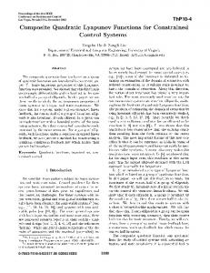
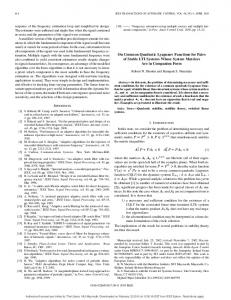
two quadratic functions even for a system that switches between two Ai ’s. To demonstrate that the switching feedback law corresponding to η4∗ is stabilizing with the guaranteed convergence rate, we run a set of simulations from different initial conditions for the system with A1 and A2 replaced with A¯1 = A1 − η4∗ I/2 and A¯2 = A2 − η4∗ I/2. It can be seen that A¯1 and A¯2 satisfy the matrix inequalities with the same parameters except that η = 0, which means that a guaranteed convergence rate is 0. A typical result is plotted in Fig. 1 which shows Vmin as a function of time and the dotted line identifies the index j such that xT Pj x = Vmin . In Fig. 2, the convergence rate V˙ /V is plotted as a function of time. The maximum value of V˙ /V is −3.773×10⁻⁴ , slightly below 0 (not exactly 0 because of sampling rate). This shows that the convergence rate is closely reflected from the matrix equations.
Claim 1: η0∗ ≥ η1∗ . Based on the stability condition in Proposition 2, an optimization problem can be formulated for the optimization of the convergence rate as follows η
(21)
15
Vmin
inf
Pj ,αij ,βjk
20
s.t. 1)(18) 2) Pj = PjT > 0, αij ∈ [0, 1], βjk ≥ 0, ΣN i=1 αij = 1.
Example 1: Consider a third-order switched system with −3 −6 3 1 3 3 2 −3 , A2 = −1 −3 −3 . A1 = 2 1 0 −2 0 0 2 Both A1 and A2 are neutrally stable. There exist no convex combination of A1 and A2 that is Hurwitz. We turn to use Vmin composed from two quadratic functions and minimize η1 subject to (20). The minimal η1 is quickly determined through the path-following algorithm as η1∗ = −0.3375. The same η1∗ is obtained by sweeping β1 and β2 in (20) from 0 to ∞. If we use Vmin composed from more quadratic functions, the convergence rate can be further increased. With J = 3, a local minimum η ∗ for the BMI problem (21) is found to be η3∗ = −0.3836. With J = 4, a local minimum η ∗ is found to be η4∗ = −0.4656. This shows that Vmin with three or more quadratic functions can work better than those with
5
P4
P3 P1
0 0
P2
5
10
15
t (sec)
Fig. 1.
Vmin as a function of time.
0.4
P4 P3
0.2 0 (dVmin/dt)/ Vmin
The matrix inequality involves bilinear terms as the product of a scalar variable and a matrix variable. They are similar to those bilinear matrix inequalities we have encountered in [7], [12] resulting from using Vc and Vmax on LDIs. Extensive numerical experience shows that a combination of the pathfollowing method in [9] and the direct iteration works very well on this type of BMI problems. We developed a twostep iterative algorithm. The first step uses the path-following method to update all the parameters at the same time. The second step fixes βjk ’s and αij ’s and solves the resulting “gevp” problem which includes only Pj ’s as variables. This procedure is repeated until the improvement is within a small range.
10
P2 P1
−0.2 −0.4 −0.6 −0.8 −1 0
5
10
15
t (sec)
Fig. 2.
The convergence rate as a function of time.
IV. S TABILIZATION VIA MAX FUNCTION AND CONVEX HULL FUNCTION
As established in [8], Vmax and Vc are conjugate types. In particular, for 1 max{xT Pj x : j ∈ I[1, J]}, 2 its conjugate function is −1 J X 1 Vc (ξ) = min ξ T γj Pj ξ. 2 γ∈ΓJ j=1 Vmax (x) =
(22)
(23)
1 1 ⇔ x ∈ ∂Vc (ξ), Vc (ξ) = . 2 2 (24) Since Vc is continuously differentiable, ∂Vc (ξ) is single valued and equals its gradient. At a point x where Vmax is not differentiable, ∂Vmax (x) is a convex set given by Lemma 1. By (24), for all ξ ∈ ∂Vmax (x), their gradient ∇Vc (ξ) = ∂Vc (ξ) = x. Based on the equivalence relation (24), a set of dual relationships are easily established in [8] for dual linear differential inclusions. For dual state-dependent switched systems, the dual relationship is complicated by the discontinuity of switch and possible sliding motion. Given A1 , A2 , · · · , AN and a pair of conjugate functions Vmax (x) and Vc (ξ). Consider the dual switched systems ξ ∈ ∂Vmax (x), Vmax (x) =
x˙ = Aσ1 (x) x,
(25)
where σ1 (x) = arg mini∈I[1,N ] V˙ max (x; Ai x), and ξ˙ = ATσ2 (ξ) ξ,
(26)
where σ2 (ξ) = arg mini∈I[1,N ] V˙ c (ξ; ATi ξ). Proposition 3: Let η ∈ R be given. The following two statements are equivalent: 1) For every x 6= 0 there exist λ ∈ ΓN such that ¢ ¢ ¡ ¡ (27) V˙ max x; ΣN i=1 λi Ai x ≤ ηVmax (x). 2) For every ξ 6= 0 there exist λ ∈ ΓN such that ¡ ¡ ¢ ¢ T V˙ c ξ; ΣN i=1 λi Ai ξ ≤ ηVc (ξ).
(28)
Conditon 2) ensures that Vc (ξ(t)) ≤ Vc (ξ(0))eηt for every solution of (26) (including sliding motion). In case N = 2, condition 1) ensures that Vmax (x(t)) ≤ Vmax (x(0))eηt for all solutions (including sliding motion) for (25). Since Vmax is piecewise quadratic and Vc is not, it seems to be easier to establish a matrix condition for (27) via the S procedure. Because of the dual relationship in Proposition 3, we can establish a matrix condition for Vc by using Vmax on the dual systems ATi . For example, consider the case N = 2 and J = 2. Using S procedure, a set of matrix inequality conditions can be established to ensure (27): there exist real numbers αij ∈ [0, 1], βjk ≥ 0, i ∈ I[1, 2], j, k ∈ I[1, 2] such that Σ2i=1 αij = 1 and (Σ2i=1 αij Ai )T Pj J X ≤
+
Pj (Σ2i=1 αij Ai )
βjk (Pk − Pj ) + ηPj
j = 1, 2,
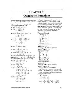
The following example demonstrates the dual relationship in Proposition 3. Example 2: Consider a second-order switched system with · ¸ · ¸ 0 0 1 2 A1 = , A2 = . −0.5 −1 −1 −1 A1 has one eigenvalue at 0 and A2 has a pair of complex eigenvalues on the imaginary axis. Let Vmax be constructed from · ¸ · ¸ 0.45 0.6 0.7 0.7 P1 = , P2 = . 0.6 1.1 0.7 0.9 The inequality (27) is satisfied for every differentiable x with η = −0.5263, as can be seen in Fig. 3, where the directional derivatives V˙ max (x; A1 x) and V˙ max (x; A2 x) are plotted along the boundary of the 1-level set LVmax from ∠x = 0 to ∠x = 2π. The solid curve corresponds to V˙ max (x; A1 x) and the dash-dotted corresponds to V˙ max (x; A2 x). Both of these curves are discontinuous. At one pair of nondifferentiable points, we have min{V˙ max (x; Ai x) : i = 1, 2} ≤ ηVmax (x). At another pair of nondifferentiable points, V˙ max (x; Ai x) > 0 for both i = 1, 2, but there exist a convex combination of A1 x and A2 x, such that V˙ max (x; (λA1 + (1 − λ)A2 x) < −0.25Vmax (x). This is also illustrated in Fig. 4, where the boundary of LVmax is plotted in thick solid curve and the directions of A1 x and A2 x are indicated by dashed line segments pointing from the boundary. At the lower-right (or upper-left) vertex of the level set, A1 x and A2 x both point outward of the level set but a convex combination of A1 x and A2 x points inward of it. By Proposition 3, the system under the corresponding switching law is stable and has a guaranteed convergence rate η1 = −0.25 even if sliding motion occurs, as confirmed by a trajectory in Fig. 4. This trajectory starts at a point marked with “∗” and enters a sliding mode on the line where xT P1 x = xT P2 x. 1 dVmax/dt(x, A1x), dVmax/dt(x, A2x)
Because of the conjugate relationship, we have
(29)
and there exist ai ∈ [0, 1], Σ2i=1 ai = 1, and bj ∈ R, dj ∈ [0, 1], j = 1, 2 such that (Σ2i=1 ai Ai )T Pj + Pj (Σ2i=1 ai Ai ) ≤ bj (P1 − P2 ) + η(dj P1 + (1 − dj )P2 ), j = 1, 2. (30) The condition (29) ensures (27) for x where xT P1 x 6= xT P2 x and (30) ensures (27) for x where xT P1 x = xT P2 x.
0 −0.5 −1 −1.5 −2 −2.5 0
Fig. 3.
k=1
0.5
1
2
3
θ=∠ x
4
5
6
7
Directional derivatives along the boundary of LVmax
By Proposition 3, we can use P1 and P2 to construct a function Vc (ξ) = min{ξ T (γP1 + (1 − γ)P2 )−1 ξ : γ ∈ [0, 1]} so that the dual switched system with AT1 and AT2 is stable and Vc (ξ(t)) has a convergence rate η1 = −0.25. This is confirmed by Figs. 5 and 6. The directional derivatives V˙ c (ξ; AT1 ξ) and V˙ c (ξ; AT2 ξ) are plotted in Fig. 5 along the boundary of the 1-level set LVc from ∠ξ = 0 to ∠ξ = 2π, where the solid curve corresponds to V˙ c (ξ; AT1 ξ) and the dash-dotted curve corresponds to V˙ c (ξ; AT2 ξ). Both
functions. Furthermore, non-convex optimization problems and tools are expected to incorporate much greater design freedoms than an overly simplified convex optimization problem. As numerical examples demonstrate in this paper, composite quadratic functions can effectively reduce the conservatism in stability conditions via solving BMI problems.
3 2
x
2
1 0 −1
A x 1
−2 −3 −3
Fig. 4.
R EFERENCES
A2x
−2
−1
0 x1
1
2
3
Boundary of the level set LVmax and a converging trajectory
of these curves are continuous and it can be seen that min{V˙ c (ξ; ATi ξ) : i = 1, 2} ≤ −0.25Vc (ξ) is satisfied for all ξ. In Fig. 6, the boundary of a level set and a trajectory starting from a point marked with “∗” are plotted. This trajectory also enters a sliding mode after some time.
dVc/dt(ξ, AT1 ξ), dVc/dt(ξ, AT2 ξ)
1 0.5 0 −0.5 −1 −1.5 −2 −2.5 0
Fig. 5.
1
2
3
θ=∠ξ
4
5
6
7
Dual system: Directional derivatives along the boundary of LVc
1.5 1
ξ2
0.5 0 −0.5 −1 −1.5 −1
Fig. 6.
−0.5
0 ξ1
0.5
1
Dual system: Boundary of LVc and a converging trajectory
V. C ONCLUSIONS The three types of Lyapunov functions studied in this paper are directly constructed from a family of quadratic functions (without additional parameters) and are natural extensions of quadratic functions. They can be used to approximate a wide variety of convex/non-convex functions which are homogeneous of degree 2. They lead to matrix inequalities as conditions for stability/stabilization. Since switched systems are intrinsically nonlinear and discontinuous, a nondifferentiable and non-convex Lyapunov function may work better than convex and/or differentiable Lyapunov
[1] M. S. Branicky, “Stability of switched and hybrid systems: State of the art,” Proc. IEEE Conf. Decision and Control, pp. 1208-1212, 1997. [2] G. Chesi, A. Garulli, A. Tesi and A. Vicino, “Homogeneous Lyapunov functions for systems with structured uncertainties,” Automatica, 39, pp. 1027-1035, 2003. [3] W. P. Dayawansa and C. F. Martin, “A converse Lyapunov theorem for a class of dynamical systems which undergo switching,” IEEE Trans. on Automat. Contr., 44, No. 4, pp. 751-760, 1999. [4] Decarlo, R.A. Branicky, M.S. Pettersson, S. Lennartson, B., “Perspectives and results on the stability and stabilizability of hybrid systems,” Proceedings of the IEEE, 88(7), pp. 1069-1082, 2000. [5] E. Feron, “Quadratic stabilizability of switched systems via state and output feedback,” Center for Intelligent Control Systems, MIT, Tech. Rep. CICS P-468, 1996. [6] A. F. Filippov, Differential Equations with Discontinuous Right Hand Sides. Norwell, MA: Kluwer Academic, 1988. [7] R. Goebel, T. Hu and A. R. Teel, “Dual matrix inequalities in stability and performance analysis of linear differential/difference inclusions,” In Current Trends in Nonlinear Systems and Control. Birkhauser, 2005. [8] R. Goebel, A. R. Teel, T. Hu and Z. Lin, “Conjugate convex Lyapunov functions for dual linear differential equations,” IEEE Transactions on Automatic Control, 51(4), pp. 661-666, 2006. [9] A. Hassibi, J. How and S. Boyd, “A path-following method for solving BMI problems in control,” Proc. of American Contr. Conf., pp. 13851389, 1999. [10] B. Hu, X. Xu, A. N. Michel, P. J. Antsaklis, “Robust stabilizing control laws for a class of second-order switched systems,” Systems & Control Letters, 38, pp. 197-207, 1999. [11] B. Hu, G. Zhai and A. N. Michel, “Common quadratic Lyapunov-like functions with associated switching regions for two unstable secondorder LTI systems Int. J. of Control, 75(14), pp. 1127-1135, 2002. [12] T. Hu, R. Goebel, A. R. Teel and Z. Lin, “Conjugate Lyapunov functions for saturated linear systems,” Automatica, 41(11), pp. 19491956, 2005. [13] T. Hu and Z. Lin, “Composite quadratic Lyapunov functions for constrained control systems,” IEEE Trans. on Automatic Control, 48, pp. 440-450, 2003. [14] D. Liberzon and A. S. Morse, “Basic problems in stability and design os switched systems,” IEEE Contr. Sys. Mag., 19(5), pp. 59-70, 1999. [15] H. Lin and P. Antsaklis, “Stability and stabilizability of switched linear systems: a short survey of recent results,” Proc. of the 2005 IEEE Int. Sym. on Intelligent control, pp. 24-29, Limassol, Cyprus, 2005. [16] A. N. Michel, “Recent trends in the stability analysis of hybrid dynamical systems,” IEEE Trans. Circuits Systems I, 46, pp. 120-134, 1999. [17] Pettersson, S., “Controller design of switched linear systems,” American Control Conf., pp. 3869-3874, 2004. [18] R. T. Rockafellar. Convex Analysis. Princeton University Press, 1970. [19] V. I. Utkin, “Variable structure systems with sliding mode,” IEEE Trans. Automat. Contr., 22(2), pp. 212-222. [20] M. A. Wicks, P. Peletics and R. A. Decarlo, “Switched controller synthesis for the quadratic stabilization of a pair of unstable linear systems,” European J. Contr. 4, pp.140-147, 1998. [21] M. Wicks and R. Decarlo, “Solution of coupled Lyapunov Equations for the stabilization of multimodal linear systems,” Proc. of the American Control Conf., pp. 1709-1713, 1997. [22] L. Xie, S. Shishkin and M. Fu, “Piecewise Lyapunov functions for robust stability of linear time-varying systems,” Sys. & Contr. Lett., 31, pp.165-171, 1997. [23] X. Xu and P. J. Antsaklis, “Stabilization of second-order LTI switched systems,” Int. J. of Control, 73, pp. 1216-1279, 2000. [24] H. Ye, A. N. Michel and L. Hou, “Stability for hybrid dynamical systems,” IEEE Trans. on Automatic Control, 43, pp. 461-474, 1998. [25] G. Zhai, H. Z. Lin, P. J. Antsaklis, “Quadratic stabilizability of switched linear systems with polytopic uncertainties,” Int. J. of Control, 76(7),pp. 747-753, 2003.