On Single-Sequence and Multi-Sequence Factorizations Lihi Zelnik-Manor Department of Electrical Engineering California Institute of Technology Pasadena, CA 91125, USA
[email protected]
Michal Irani Department of Computer Science and Applied Math The Weizmann Institute of Science Rehovot, 76100, Israel
[email protected]
http://www.vision.caltech.edu/lihi/Demos/MultiSeqFactorization.html
Abstract Subspace based factorization methods are commonly used for a variety of applications, such as 3D reconstruction, multi-body segmentation and optical flow estimation. These are usually applied to a single video sequence. In this paper we present an analysis of the multi-sequence case and place it under a single framework with the single sequence case. In particular, we start by analyzing the characteristics of subspace based spatial and temporal segmentation. We show that in many cases objects moving with different 3D motions will be captured as a single object using multi-body (spatial) factorization approaches. Similarly, frames viewing different shapes might be grouped as displaying the same shape in the temporal factorization framework 1 . We analyze what causes these degeneracies and show that in the case of multiple sequences these can be made useful and provide information for both temporal synchronization of sequences and spatial matching of points across sequences.
1
Introduction
When a single video camera views a dynamic scene we are interested in two different segmentation tasks: (i) Separate spatially between objects moving with different motions. We refer to this as the “multi-body factorization problem”, which was presented in [3, 4]. (ii) Separate temporally between frames which capture different rigid shapes, i.e., “temporal factorization” [14]. When multiple video cameras view the same scene at the same time, in addition to the segmentation problems, we are interested also in matching across cameras. This can be either temporal matching (i.e., temporal synchronization) or spatial matching (i.e., point correspondences). We refer to this as the “multi-sequence factorization problem”. The body of work on multi-body factorization (e.g., [3, 4, 5, 1, 8]), suggest employing multi-frame linear subspace constraints to separate between objects moving with independent motions. We first show that often objects moving with different 3D motions will be captured as a single object using previously suggested approaches. We show that this happens when there is partial linear dependence between the object motions. In many of these cases, although the motions are partially dependent they are conceptually different and we would like to separate them. We use equivalent arguments to reveal degeneracies in temporal factorization. Previous work on temporal factorization utilized multi-frame linear subspace constraints to group frames viewing the same rigid shape [14]. This results in a temporal segmentation where cuts are detected at non-rigid shape changes. For example, in a sequence showing a face smiling and serious intermittently temporal factorization will group together all the “smiling” frames separately from all the “serious” frames. In this paper we show that just like dependence between motions can result in degeneracies in spatial segmentation, dependence between shapes can result in frames viewing different shapes being captured as displaying the same shape. 1 Temporal factorization provides temporal grouping of frames by employing a subspace based approach to capture non-rigid shape changes [14].
1
Interestingly, the same dependence which causes degeneracies in the single-sequence segmentations can become useful in the multi-sequence case. When multiple video sequences of the same dynamic scene are available (which includes either a single object or multiple objects) there can also be dependence between the motions or shapes captured by the sequences. A first attempt toward utilizing such dependence was suggested by Wolf & Zomet [12] who showed that a dependence between the motions can be used for temporal synchronization of sequences. We extend their analysis and show that even partial dependence suffices for synchronization purposes. This can be applied to synchronize sequences with only partially overlapping fields of view. Moreover, we show that when the sequences share some spatial overlap one gets a dependence which can be often used to find the spatial matching of points across sequences. For completeness of the text we additionally suggest a method for separating objects/frames in the singlesequence case, even for cases which are degenerate and non-separable by previous methods. The rest of the paper is organized as follows. In Section 2 we define the the types of dependence of interest and explore what causes them. Then, in Sections 3 and 4 we show that some of cases of dependence can result in a wrong spatial or temporal segmentation. In Section 5 we present the multi-sequence case and show how the same types of dependence can be made useful. Finally, an approach to segmentation under such degenerate cases is suggested in Section 6. A preliminary version of this paper appeared in [13].
2
Dependence between Image Coordinate Matrices
Let I1 , . . . , IF denote a sequence of F frames with N points tracked along the sequence. Let (x fi , yif ) denote the coordinates of pixel (xi , yi ) in frame If (i = 1, . . . , N , f = 1, . . . , F ). Let X and Y denote two F × N matrices constructed from the image coordinates of all the points across all frames:
x11 2 x1
X=
xF1
x12 x22
· · · x1N · · · x2N .. .
xF2
· · · xFN
y11 2 y1
Y =
y1F
y21 y22
1 · · · yN 2 · · · yN .. .
y2F
F · · · yN
(1)
Each row in these matrices corresponds to a single frame, and each column corresponds to a single point. Stacking · ¸ X the matrices X and Y of Eq. (1) vertically results in a 2F × N matrix . It has been previously shown that Y under various camera and scene models2 [10, 6, 2] the image coordinate matrix of a single object can be factorized · ¸ X into motion and shape matrices: = M2F ×r Sr×N . When the scene contains multiple objects (see [3, 4]) we Y · ¸ X = Mall Sall where Mall is the matrix of motions of still get a factorization into motion and shape matrices Y all objects and Sall contains shape information of all objects. A similar factorization was also shown for the horizontally stacked matrix, i.e., [X, Y ] [7, 2, 9]. To simplify · ¸ X the text we start by showing results only for the matrix case. In Section 2.2 we present the [X, Y ] case and Y analyze its characteristics. ¸ · X1 and Let W1 (of size 2F1 × N1 ) and W2 (of size 2F2 × N2 ) be two image coordinate matrices ( W1 = Y1 · ¸ X2 W2 = ). In the case of the multi-body single sequence factorization, each of these would correspond to an Y2 2
In general once could say the following factorization holds for affine cameras and not for perspective ones. Nevertheless, it has been utilized successfully for applications like motion based segmentation and 3D reconstruction on a variety of sequences taken by off-the-shelf cameras, e.g., [10, 6, 4, 2, 9].
2
independently moving object, i.e., W1 = Wobj1 , W2 = Wobj2 . The objects can have a different number of points, i.e., N1 6= N2 but are tracked along the same sequence such that F1 = F2 . In the case of temporal factorization (single sequence) each of these matrices would correspond to a subset of frames viewing an independent shape, i.e., W1 = Wf rames1 and W2 = Wf rames2 . Both frame subsets view the same number of points N1 = N2 but can be of different lengths, i.e., F1 6= F2 . Finally, in the case of multi-sequence factorization, each of these matrices corresponds to a single sequence (i.e., the trajectories of all points on all objects in each sequence): W 1 = Wseq1 and W2 = Wseq2 . Here both the number of points and the number of frames can be different across sequences. Let r1 and r2 be the true (noiseless) ranks of W1 and W2 , respectively. Then, in all three cases (i.e., multi-body, temporal and multi-sequence factorization) these matrices can be each factorized into motion and shape information: [W1 ]2F1 ×N1 = [M1 ]2F1 ×r1 [S1 ]r1 ×N1 and [W2 ]2F2 ×N2 = [M2 ]2F2 ×r2 [S2 ]r2 ×N2 , where M1 , M2 contain motion information and S1 , S2 contain shape information. In the multi-sequence factorization case the motion and shape matrices will include information of all the objects across all frames in the corresponding scene. In this paper we will examine the meaning of full and partial linear dependence between W 1 and W2 , and its implications on multi-body, temporal (single sequence) and multi-sequence factorizations. We will see that in the single sequence case this dependence leads to degeneracies (and therefore is not desired), whereas in the multi-sequence factorization this dependence is useful and provides additional information. In particular, there are two possible types of linear dependence between W1 and W2 : (i) Full or partial linear dependence between the columns of W1 and W2 , and (ii) Full or partial linear dependence between the rows of W 1 and W2 . We will show that: 1. In the multi-body factorization case: - Dependence between the columns of W1 and W2 causes degeneracies and hence misbehavior of multibody segmentation algorithms. - Linear dependence between the rows has no effect on the multi-body factorization. 2. In the temporal factorization case: - Dependence between the rows of W1 and W2 causes degeneracies and hence misbehavior of temporal factorization algorithms. - Linear dependence between the columns has no effect on the temporal factorization. 3. In the multi-sequence factorization case: - Linear dependence between the columns of W1 and W2 (assuming F1 = F2 ) provides constraints for temporal correspondence (i.e., temporal synchronization) between sequences. - Linear dependence between the rows of W1 and W2 (assuming N1 = N2 ) provides constraints for spatial correspondence (i.e., spatial matching of points) across the sequences.
2.1 Definitions and Claims Before we continue we need to mathematically define what we mean by full and partial dependence between matrices. We outline the definitions for dependence between column spaces. Equivalent definitions on the row spaces can be easily derived and are thus omitted. Let π1 , π2 be the linear subspaces spanned by the columns of W1 and W2 , respectively, and r1 and r2 be the ranks of W1 and W2 , respectively (i.e., r1 = rank(W1 ) and r2 = rank(W2 )). The two subspaces π1 and π2 can lie in three different configurations: 1. Linear Independence: When π1 and π2 are two disjoint linear subspaces π1 ∩π2 = {0} and rank([W1 |W2 ]) = r1 + r 2 . 2. Full Linear Dependence: When one subspace is a subset of (or equal to) the other (e.g., π 2 ⊆ π1 ), then W2 = W1 C and rank([W1 |W2 ]) = max(r1 , r2 ). 3. Partial Linear Dependence: When π1 and π2 intersect partially ({0} ⊂ π1 ∩π2 ⊂ π1 ∪π2 ), then max(r1 , r2 ) < rank([W1 |W2 ]) < r1 + r2 . 3
The analysis in the following sections will be based on the following two claims on the full/partial dependence between the columns and between the rows of W1 and W2 . The proofs of these claims are provided in the Appendix. Claim 1 Let F1 = F2 . The columns of W1 and W2 are fully/partially linearly dependent iff the columns of M1 and M2 are fully/partially linearly dependent. Note, that in the case of full linear dependence this reduces to: ∃C s.t. W2 = W1 C iff ∃C 0 s.t. M2 = M1 C 0 (C is a N1 × N2 coefficient matrix, and C 0 is a matrix of size r1 × r2 which linearly depends on C). Claim 2 Let N1 = N2 . The rows of W1 and W2 are fully/partially linearly dependent iff the rows of S1 and S2 are fully/partially linearly dependent. Note, that in the case of full linear dependence this reduces to: ∃C s.t. W2 = CW1 iff ∃C 0 s.t. S2 = C 0 S1 (C is a N2 × N1 coefficient matrix, and C 0 is a matrix of size r2 × r1 which linearly depends on C).
2.2 The [X, Y ] case As discussed in the previous section one can obtain a factorization into motion and shape also for the horizontally stacked matrix, i.e., W = [X, Y ] = M S (see [7, 2, 9]). These matrices are of different dimensions: W = [X, Y ] is of size F × 2N , the motion matrix M is of size F × r and the shape matrix is of size r × 2N · ¸ X case. Nevwhere r is their actual rank. The rank r can also be different from the rank of the matrices in the Y ertheless, all the claims and observations regarding linear dependence of Section 2 hold also for the [X, Y ] case. This is since the meaning of dependence between rows or columns does not depend in any way on the dimensions of the image coordinate matrix matrix W nor on the dimensions of the motion and shape matrices. In the following sections we examine the meaning and the implications of each of these types of dependence, both for the single-sequence case (multi-body and temporal factorizations) and for the multi-sequence case.
3
Single Sequence Multi-Body Factorization
We next examine the implications of linear dependence between the columns or rows of W 1 and W2 (of obj1 and obj2) on the familiar multi-body factorization problem. We show (Section 3.1) that full or partial dependence between the columns of W1 and W2 result in grouping together of objects while a dependence between the rows of W1 and W2 has no effect on the segmentation (Section 3.2).
3.1 Dependence Between Object Motions Let W1 (of size 2F × N1 ) and W2 (of size 2F × N2 ) be the image coordinates sub-matrices corresponding to two objects (W1 = Wobj1 and W2 = Wobj2 ) across F frames. We wish to classify the columns of the combined matrix [W1 |W2 ] according to objects. Let π1 , π2 be the linear subspaces spanned by the columns of W1 and W2 , respectively, and r1 and r2 be the ranks of W1 and W2 , respectively (i.e., r1 = rank(W1 ) and r2 = rank(W2 )). The subspaces π1 and π2 which are spanned by the columns of W1 and W2 , respectively, can lie in three different configurations: I. Linear Independence: When the columns of W1 and W2 are linearly independent, then according to Claim 1 the motions M1 and M2 of the two objects are linearly independent as well. Algorithms for separating independent linear subspaces can separate the columns of W1 and W2 . II. Full Linear Dependence: When the columns of W1 and W2 are fully linearly independent, then according to Claim 1 the motions M1 and M2 of the two objects are fully linearly dependent as well, i.e., M 2 = M1 C 0 . In this case all subspace based algorithms should group together the columns of W 1 and W2 . III. Partial Linear Dependence: When the columns of W1 and W2 are partially linearly independent, then according to Claim 1 the motions M1 and M2 of the two objects are partially linearly dependent as well. In this 4
(a)
(d)
(b)
(e)
(c)
(f)
(g)
Figure 1. Degeneracies in multi-body (single sequence) factorization: (a)-(c) Sample frames (at
times t=1,17,34) from a synthetic sequence showing partially dependent objects (tracked points marked in black). Both objects rotate counter-clockwise, but the yellow anchor also translates horizontally whereas the cyan cross translates vertically. (d) The distance matrix used by previous algorithms for segmentaˆ tion (the “shape interaction matrix” Q) after sorting the points according to objects. (e) The matrix Q we suggest to use, after sorting the points according to objects. (f) Segmentation into two objects when using the classical shape interaction matrix Q. Points in differently detected clusters are marked by different markers (circles and triangles) and colors (red and blue). The segmentation is obviously erroneous and mixes between the objects. (g) The corresponding segmentation result when using our proposed maˆ The points on the red and the cyan objects are separated correctly. Video can be viewed at trix Q. http://www.vision.caltech.edu/lihi/Demos/MultiSeqFactorization.html
case subspace based approaches can in general separate between the objects, however, most previously suggested algorithms will group them into a single object. This is explained next. Costeira and Kanade [3] have estimated the SVD of [W1 |W2 ], i.e., [W1 |W2 ] = U ΣV T (where U and V are · T −1 ¸ S 1 Λ1 S 1 0 unitary matrices) and showed that the “shape interaction matrix” Q = V V T = has a 0 S2T Λ−1 2 S2 block diagonal structure. The algorithm they suggested (as well as those suggested in [3, 5, 1, 8]) relied on the block diagonal structure of Q which occurs if and only if V is block diagonal. However, the columns of V are ¸ · T T S1 M1 M1 S1 S1T M1T M2 S2 T . Hence, V and therefore Q will have the eigenvectors of [W1 |W2 ] [W1 |W2 ] = S2T M2T M1 S1 S2T M2T M2 S2 a block diagonal structure if and only if the motion matrices M 1 and M2 are linearly independent. When M1 and M2 are partially dependent the off-diagonal blocks S1T M1T M2 S2 and S2T M2T M1 S1 are non-zero. Algorithms like [3, 5, 1, 8], which rely on the block diagonal structure of Q will fail to separate between the objects. Note, that partial dependence occurs even if only a single column of the motion matrix of one object is linearly dependent on the columns of the motion matrix of the other object. This can occur quite often in real sequences. An example for this is given in Fig. 1. The synthetic sequence displays a planar scene with two objects (a yellow anchor and a cyan cross) moving with the same rotations but with independent translations. Putting together all the image coordinates of all points corresponding to the yellow anchor yields a matrix W anchor where rank(Wanchor ) = 3. Similarly, the matrix of image coordinates of the cyan cross has rank(W cross ) = 3. Combining the image coordinates of all points on both objects into a single matrix gives W = [W anchor |Wcross ] with rank(W ) = 4. This implies that the column subspaces corresponding to the yellow anchor and to the cyan cross 5
(a)
(b)
(c)
(d)
(e)
Figure 2. Degeneracies in temporal factorization: (a)-(b) Sample frames (at times t=1,30) from a synthetic
sequence showing a smiley face, with two different expressions, translating and rotating in the image plane. (c) An overlay of the points in the two expressions shows that the non-rigid transformation between the two expressions is only in the vertical direction. (d) The distance matrix used by previous algorithms for segmentation after sorting the frames according to expressions. (e) The matrix we suggest to use, after sorting the frames according to expressions. Now the block diagonal structure is evident. Video can be viewed at http://www.vision.caltech.edu/lihi/Demos/MultiSeqFactorization.html
intersect. Fig. 1.d shows that the matrix Q has no block-diagonal structure. Therefore, most previous subspace based segmentation algorithms will group the two objects as one although their motions are obviously different.
3.2 Dependence Between Object Shapes As was shown in Section 2, a dependence between the rows of W 1 and W2 implies that S2 = C 0 S1 . This implies that both objects share the same shape up to a selection of the object coordinate frame. When only the shapes are dependent and the motions are still independent, the two objects will still be separated in all multi-body " # segmentation algorithms, since: S1 0 [W1 |W2 ] = [M1 |M2 ] 0 CS1 and rank([W1 |W2 ]) = r1 + r2 . We can conclude and say that a dependence between the rows of W 1 and W2 has no effect on the multi-body segmentation.
4
Single Sequence Temporal Factorization
In the case of temporal factorization our goal is to group frames viewing the same shape separately from frames viewing different shapes. For example one would like to group frames according to expression (see [14] for more details). Here the matrices W1 = Wf rames1 and W2 = Wf rames2 correspond to the same N points tracked along a single sequence with F 1 frames displaying one configuration of the points (e.g., “smile” expression) and F 2 frames displaying a different configuration of the points (e.g., “angry” expression) 3 . We wish to classify the rows ¸ · W1 according to shape. As was shown in [14], when the shapes captured by the two of the combined matrix W2 frame subsets are independent the obtained factorization results in a motion matrix with a block diagonal structure: M1 W1 = W = W2 0 ·
¸
·
0 M2
¸·
S1 S2
¸
The analogy to the multi-body factorization case can be seen if one takes the transpose of that matrix: W T = [ W1T
W2T ] = [ S1T
3
S2T ]
·
M1T 0
0 M2T
¸
In the case of temporal factorization, since the grouping is on frames and not on points, it is more natural to use the matrices W 1 = Wf rames1 = [X1 , Y1 ] of size F1 × 2N and W2 = Wf rames2 = [X2 , Y2 ] of size F2 × 2N . As was shown in Section 2.2 all our claims and observations hold for these matrices just as well, thus the analysis is the same.
6
That is, the matrix W T can be factored into a product of two matrices where the matrix on the right is block diagonal. This is equivalent to the assumption made in the multi-body factorization case to obtain column clustering. Zelnik-Manor and Irani [14] used this observation to separate between frames corresponding to independent shapes. They showed that one can use any of the algorithms suggested for multi-body segmentation, but applying them to the matrix W T instead of W . The duality to the multi-body factorization case implies also a dual effect of dependence between motions and shapes on temporal factorization. We next show that in the temporal factorization case dependence between motions will have no effect whereas dependence between shapes will result in a wrong segmentation.
4.1 Dependence Between Motion Across Frames As was shown in Section 2 dependence between the columns of W 1 and W2 implies that M2 = M1 C 0 while the shapes S1 and S2 are independent. This corresponds to different frames capturing different shapes, but moving with the same motion (up to a selection of the coordinate frame). We can thus write M1 W1 = W = W2 0 ¸
·
and rank(
·
·
0 M1 C 0
¸·
S1 S2
¸
W1 ) = r1 + r2 . The two frame subsets can still be separated in all subspace based algorithms. W2 ¸
4.2 Dependence Between Shapes Across Frames Unfortunately, a different result is obtained for dependence between shapes. As was shown in Section 2 dependence between the rows of W1 and W2 implies that S2 = C 0 S1 , i.e., both frame subsets capture the same shape up to a selection of the coordinate frame. In that case we can write W1 M1 W = = [ S1 ] W2 M2 C 0 ·
¸
·
¸
and the two frame subsets will be grouped together as capturing the same shape. As in the case of multi-body factorization, partial dependence will completely destroy the block diagonal structure just as well. This is illustrated in Figure 2. The synthetic video sequence shows a smiley face in two different expressions, smiling and sad (Figures 2.a,b). The non-rigid transformation between the two expressions was obtained by fixing the x coordinate of all the points while changing the y coordinate of only the mouth points (see Figure 2.c). The matrix Q, which is the equivalent to the “shape interaction matrix” only obtained using W T instead of W , has no block diagonal structure and thus contains no information for segmentation (Figure 2.d).
5
Multi-Sequence Factorization
In the previous sections it was shown that linear dependence between motions or shapes within a single sequence can lead to wrong segmentations. In this section we shift to the multi-sequence case and show that as opposed to the single-sequence case, here dependence between the image coordinate matrices W 1 and W2 of the two sequences does not cause degeneracies. On the contrary, it produces useful information! In particular, dependence between the columns of W1 and W2 supplies information for temporal synchronization of the sequences (Section 5.1) and dependence between the rows of W1 and W2 supplies information for spatial matching of points across sequences (Section 5.2). The multi-sequence case was previously discussed by Torresani et al. [11]. There it was shown that given the temporal synchronization of the sequences and the spatial matching of points across the sequences one can apply 3D reconstruction using the data from all the sequences simultaneously. The analysis and applications suggested in this section aim at finding these required temporal and spatial matchings. As we next examine the case of multiple sequences, we will denote by W 1 = Wseq1 = Mseq1 Sseq1 and W2 = Wseq2 = Mseq2 Sseq2 the image coordinate matrices corresponding to separate video sequences. Each 7
sequence can contain multiple objects moving with different motions and the corresponding motion and shape matrices will include information of all the objects in the scene. We further wish to remind the reader that the linear analysis suggested here applies only to affine cameras and thus the applications described next apply in theory only to sequences for which the affine assumption holds.
5.1 Temporal Synchronization Wolf & Zomet [12] showed how subspace constraints can be used for temporal synchronization of sequences when two cameras see the same moving objects. We reformulate this problem in terms of dependence between W1 and W2 , and analyze when this situation occurs. We further extend this to temporal synchronization in the case of partial dependence between W1 and W2 (i.e., when the fields-of-view of the two video cameras are only partially overlapping). As was shown in Claim 1, the columns of W1 and W2 are linearly dependent4 when M2 = M1 C 0 . Stacking W1 and W2 horizontally gives [W1 |W2 ] = M1 [S1 |C 0 S2 ] and therefore rank ([W1 |W2 ]) ≤ r1 . Note, however, that we get this low rank only when the rows of W1 correspond to frames taken at the same time instance as the frames of the corresponding rows of W2 . This can be used to find the temporal synchronization between the two sequences, i.e., the alignment of rows with the minimal rank gives the temporal synchronization [12]. Furthermore, even if the motions that the two sequences capture are only partially linearly dependent, we will still get the lowest rank when the rows of the matrices W1 and W2 of the two sequences are correctly aligned temporally. Partial dependence between the motions captured by different sequences occurs when the fields of view of the corresponding cameras have only partial spatial overlap. Note that the cameras are assumed to be fixed with respect to each other (they can move jointly, however), but the points on the objects need not be the same points in both sequences (shape matrices can be independent). 5.1.1 Synchronization Results Figures 3,4 show temporal synchronization results on real sequences. In both examples two stationary cameras viewed the same scene but from different view points and were not activated at the same time. We tested the rank of the combined matrix [W1 |W2 ] for all possible temporal shifts. The rank was approximated by looking at the rate of decay of the singular values. Let σ1 ≥ σ2 ≥ σ3 , . . . be the singular values of [W1 |W2 ]. We set rank([W1 |W2 ]) = i − 1 where i is the index of the largest singular value for which σ i /σ1 < 0.01. Since the data is noisy we might get this rank for more than one shift. Hence, we additionally estimated the residual error P as Error = N i=rank+1 σi . The temporal shift yielding minimal rank and minimal residual error is detected as the synchronizing temporal shift. Using this method the correct temporal shifts were recovered in both examples of Figure 3 and 4. Note, that we obtained the correct result even though the points tracked in each sequence were different and only some of them were on the same objects. Note, that this multi-sequence low-dimensionality constraint can be viewed as a behavior (motion) based distance measure between sequences. That is, even for sequences viewing different scenes, the matrix [W 1 , W2 ] will have minimal rank when the two sequences capture the same motions, i.e., the same behavior / action. This is illustrated in Figure 5 where two sequences showing different people dancing were synchronized so that their dance would be in phase. 5.1.2 Synchronization Using
h
X Y
i
vs. [XY ]
Wolf & Zomet [12] have used a somewhat similar approach to temporally synchronize sequences. In their paper they used a different notation, however, one can show that their algorithm was based on finding the temporal 4
Here we implicitly assume that W1 and W2 have the same number of rows, i.e., the same number of frames. Since the sequences are obtained by different cameras this might not be true. In such cases, we take from each input sequence only a subset of F frames so that W1 and W2 will be of the same row size.
8
shift which provides the minimal rank of the matrix [X1, Y 1, X2, Y 2]. This is different from our approach in · ¸ · ¸ Xi X1 X2 which Wi = , i.e., we search for the minimal rank of the matrix . This difference is significant Yi Y1 Y2 as we explain next. Machline et al. [9] showed that when using the horizontally stacked matrix W = [X, Y ] points fall into the same subspace (and therefore are grouped together in a segmentation process) when they move with consistent motions along time, even if their motions are different. This was shown to be useful for grouping points on non-rigid objects. However, for the task of temporal synchronization we are interested in capturing the same motions and not different yet consistent ones. This is illustrated in Figure 3.b where the suggested temporal synchronization scheme was applied to the [X1, Y 1, X2, Y 2] matrix and provided a wrong result. 5.1.3 Temporal Synchronization Summary To summarize, the suggested approach to temporal synchronization has three useful properties: • The points tracked in each of the sequences can be different points as long as they share the same motion. • This approach can be applied to sequences with only partially overlapping fields of view. • The number of tracked points can be very small. For example, in Figure 3 only 12 points on the arm and leg tracked in one sequence and 15 points, on the arm, leg and head tracked in the second sequence (not the same points in both sequences) were sufficient to obtain the correct temporal synchronization between the two sequences.
5.2 Spatial Matching When the video cameras are not fixed with respect to each other but they do view the same set of 3D points in the dynamic scene, the spatial correspondence between these points across sequences can be recovered. In this case the subspaces spanned by the rows of W1 and W2 are equal5 , i.e., W2 = CW1 . As was shown in Section 2, this occurs if and only if S2 = CS1 . Note, that in this case there is no need for the cameras to be fixed with respect to each other (they can move independently), as only dependence between shapes (S 1 and S2 ) is assumed. · ¸ · ¸ µ· ¸¶ W1 M1 W1 Stacking W1 and W2 vertically gives: = S and rank ≤ max(r1 , r2 ). Note, that W2 M2 C 0 1 W2 we get this low rank only when the columns of W1 and W2 correspond to the same points and are ordered in the same way. This can be used to find the spatial correspondence between the points in the two cameras, i.e., the ¸ · W1 gives the correct spatial matching. permutation of columns in W2 which leads to a minimal rank of W2 Fig. 6.a examines this low rank constraint on the two sequences of Fig. 7. The graph shows the residual error for 1000 permutations, 999 of which were chosen randomly, and only one was set to be the correct permutation · ¸ PN W1 (the residual error here is again Error = i=rank+1 σi , where σi are the singular values of ). The graph W2 shows that the correct permutation yields a significantly lower error. We next suggest a possible algorithm for obtaining such a spatial matching of points across sequences. However, the cross-sequence matching constraint presented above is not limited to this particular algorithm. One could, for example, start by selecting r point matches (r = max(r1 , r2 )) either manually or using an image-to-image feature correspondence algorithm (taking only the r most prominent matches). The rest of the points could be matched · match ¸ W1 of the already matched points automatically by employing only temporal information: given the matrix W2match 5 Here we implicitly assume that W1 and W2 have the same number of columns, i.e., the same number of points. Since these are obtained by different cameras this might not be true. In such cases, we take from each input sequence only a subset of N points so that W 1 and W2 will be of the same column size.
9
−3
8
x 10
0.015
7.5 0.014
7
0.013
Error
Error
6.5
6
0.012
5.5 0.011
5 0.01
4.5
(a)
4 −20
−15
−10
−5
0
5
10
Size of temporal shift
(c)
15
20
(b)
0.009 −20
−15
−10
−5
0
5
10
15
20
Size of temporal shift
(d)
(e)
Figure 3. Temporal synchronization applied to the sequences of Fig. 7. Here different points were tracked in
each sequence (also different from those tracked in Figure 7), some on body-parts viewed in both sequences (e.g., leg) and some viewed in only one · sequence ¸ (e.g., face). (a) The rank residual error (see Section 5.1) for X1 X2 all temporal shifts using the matrix . The minimal error is obtained at the correct temporal shifts, Y2 Y2 which was 14 frames. (b) The residual error for all temporal shifts using the matrix [X1, Y 2, X2, Y 2]. The minima is obtained at a wrong temporal shift of -20 frames. (c) The 46’th frame of the first sequence. (d) The 46’th frame of the second sequence. As the second camera was turned on approximately half a second before the first one, this does not correspond to the 46’th frame of the first sequence. (e) The 60’th frame from the second sequence, which was recovered as the correct temporally corresponding frame to (c) (i.e., a shift of 14 frames).
we add a new point (a new column) by choosing one point from the first sequence and testing the residual error when matching it against all the remaining points from the second sequence. The match which gives the minimal residual error is taken as the correct one. Fig. 6.b illustrates that using this approach the correct spatial matching was found for the sequences of Figure 7.
6
Handling Partial Dependence
As was shown by the examples in Figures 1 and 2 in many cases one would like to separate between subspaces with partial dependence. For completeness of the text we next suggest an approach to doing so. To simplify the explanations the description is given only for the multi-body factorization case, i.e., the case of separating between objects with different motions. For the temporal factorization case one can use the same algorithm but apply it to the transposed matrix (as was shown in Section 4). The approach we suggest is similar to that suggested by Kanatani [8] which groups points into clusters in an agglomerative way. In Kanatani’s approach the cost of grouping two clusters was composed of two factors. The first factor is based on the increase in the rank when grouping the two clusters. Although intended for independent objects, this applies also to the case of partially dependent objects. This is because adding to a group of points of one object more points from the same object will not change the rank (i.e., when the initial group of points spans the linear subspace corresponding to that object), whereas adding even a single point from another object 10
First sequence:
(a)
Second sequence:
(b) 0.02
0.018
Error
0.016
0.014
0.012
(d)
0.01
0.008
(c)
0.006 −20
−15
−10
−5
0
5
Size of temporal shift
10
15
20
(e)
(f)
Figure 4. (a) Three sample frames (at times t=1, 31, 200) from a sequence showing a car in a parking lot. The tracked points are marked in yellow. (b) Frames taken at the same time instances (i.e., at times t=1, 31, 200) by the second camera. The tracked points are different form those in the other sequence. (c) Error graph for all possible temporal shifts (see Section 5). The resulting temporal shift, which yields minimal error, is 6 frames. (d) A close-up on the gate in frame t=400 of the first camera shows it is just opening. (e) A close-up on the gate in frame t=400 from the second camera shows it is still closed since the cameras are not synchronized. (f) A close-up on the gate in frame t=406 from the second camera shows that it is just opening, as in frame t=400 of the first camera, implying that a temporal shift of 6 frames synchronizes the cameras.
11
(a)
(b)
(c)
(d)
0.019
0.018
0.017
Error
0.016
0.015
0.014
0.013
0.012
(e)
0.011 −40
−30
−20
−10
0
10
20
30
Size of temporal shift
40
(f)
(g)
Figure 5. (a)-(b) Two sample frames (at times t=15, 40) from a 100 frame long sequence showing a man
shaking his butt. The tracked points are marked in yellow. (c)-(d) Two sample frames (at times t=15, 40) from a 100 frame long sequence showing a woman shaking her butt. Again, tracked points are marked in yellow. The butt motions in the two sequences are not synchronized. (e) Error graph for all possible temporal shifts (see Section 5). The resulting temporal shift, which yields minimal error, is -37 frames. Since butt shaking is a cyclic motion the second minima, at a shift of 22 frames corresponds to another possible synchronization. (f)-(g) Frame t=3 and t=62 of the woman sequence, both show her in the same pose as the man in frame t=40 (displayed in (b)). This implies that both a temporal shift of -37 frames and of 22 frames synchronize the sequences. Video can be viewed at http://www.vision.caltech.edu/lihi/Demos/MultiSeqFactorization.html
12
0.03
0.025
Error
0.02
0.015
0.01
0.005
(a)
0
0
200
400
600
Permutations
800
1000
(b)
Figure 6. Spatial matching across sequences. Spatial matching applied to the sequences of Fig. 7. (a)
The residual error for 1000 different pairings of the features across the two sequences (see Section 5.2). All wrong pairings give high residual error (i.e., high rank), whereas the correct pairing (marked by a red arrow) gives a small residual error (i.e., low rank). The correctly recovered pairing of feature points across the two sequences is shown in (b).
will increase the rank, even if the objects are only partially dependent. When the clusters are large enough the agglomerative process is likely to continue correctly, however, for the initial stages to be correct we need additional information. For this, Kanatani [8] used a second factor which is based on the values within the shape interaction matrix Q (high values indicate low-cost whereas low values indicate a high-cost). However, as was shown in Section 3.1, when the objects are partially dependent, the Q matrix looses its block diagonal structure. Hence, ˆ defined next. relying on this factor can lead to erroneous segmentation. Instead, we use the matrix Q T As was shown in Section 3, to construct the matrix Q = V V one computes the Singular Value Decomposition W = U ΣV T . The columns of U span the columns of the corresponding motion matrix, and the rows of V are the coefficients multiplying the singular vectors in U . When the dependence between the objects’ motions is partial there will still be at least K vectors in U , where K is the number of objects, each corresponding to the motion of a single object only. Therefore, there will be K vectors in V which do capture the independent part between the ˆ = Vdom V T objects. We thus suggest using only the K most dominant vectors of V to construct the matrix Q dom where Vdom = [v1 , . . . , vK ] and K is the number of objects. This is different from the standard shape interaction matrix Q which is constructed using all vectors hence has no block diagonal structure. Note, that we have assumed that the dominant vectors are those which capture the independence between the objects. While this heuristic is ˆ Since Q ˆ is used only as not always true, we are most likely to capture at least some of the required structure in Q. an additional constraint in the agglomerative clustering process this can suffice to obtain a correct segmentation in the case of partial dependence. Nevertheless, we acknowledge that in some cases it might fail. ˆ for the synthetic sequence of Figs. 1.a-c. It can be seen that Q ˆ has an obvious block Fig. 1.e shows the matrix Q diagonal structure, whereas Q does not. A similar result is shown in Figure 2.e for the temporal factorization of the sequence of Figures 2.a,b. Figures 1.f,g show a comparison of the agglomerative clustering algorithm described above, once using the ˆ Using Q ˆ gave correct segmentation results, whereas using Q mixed the matrix Q, and once using the matrix Q. points of the two objects. Fig. 7 shows an example of partial dependence in a real sequence. In this example, two cameras viewed a person stepping forward. The non-rigid motion performed by the person can be viewed as a group of rigid subparts each moving with a different motion. In both sequences we tracked points on two sub-parts: the arm and the shin (lower leg). The tracked points are marked in yellow in Figs. 7.a-c,d-f. In both sequences the rank of the image-coordinate matrix W = [W1 |W2 ] for all the points on both parts is higher than the rank of the
13
image-coordinate matrix Wi (i = 1, 2) for each of the individual parts but is lower than the sum of them, i.e., rank(Wi ) < rank([W1 |W2 ]) < rank(W1 ) + rank(W2 ) (see Fig. 7.g). Fig. 7.h and Fig. 7.i show the result of applying this clustering scheme to the points tracked in the sequences of Figs. 7.a-c and Figs. 7.d-f, respectively. The results of the segmentation (forcing it into two objects) show that the points on the arm and the shin were all classified correctly to the two different body parts.
7
Conclusions
In this paper we presented an analysis of linear dependence and its implications on single sequence (multi-body and temporal) and multi-sequence factorizations. These are summarized in the following table: Dependence between: Motions Shapes Implications on Wrong spatial Wrong temporal single sequence: segmentation segmentation Implications on Useful for Useful for spatial multiple sequences: temporal synchronization matching (across sequences) Our contributions are: • A single unified framework for analyzing single-sequence and multi-sequence factorization methods. • An analysis of degeneracies in single sequence multi-body and temporal factorizations. • An approach to separating objects/frames in such degenerate cases. • An approach to temporal synchronization even under partially overlapping fields of view. • An approach to spatial matching of points across sequences.
References [1] T.E. Boult and L.G. Brown. Factorization-based segmentation of motions. In in Proc. of the IEEE Workshop on Motion Understanding, pages 179–186, 1991. [2] C. Bregler, A. Hertzmann, and H. Biermann. Recovering non-rigid 3d shape from image streams. In IEEE Conference on Computer Vision and Pattern Recognition, volume II, pages 690–696, 2000. [3] J. Costeira and T. Kanade. A multi-body factorization method for motion analysis. In International Conference on Computer Vision, pages 1071–1076, Cambridge, MA, June 1995. [4] C.W. Gear. Multibody grouping from motion images. International Journal of Computer Vision, 2(29):133– 150, 1998. [5] N. Ichimura. A robust and efficient motion segmentation based on orthogonal projection matrix of shape space. In IEEE Conference on Computer Vision and Pattern Recognition, pages 446–452, South-Carolina, June 2000. [6] M. Irani. Multi-frame correspondence estimation using subspace constraints. International Journal of Computer Vision, 48(3):173–194, July 2002. A shorter version appeared in ICCV’99. [7] M. Irani and P. Anandan. Factorization with uncertainty. In European Conference on Computer Vision, pages 539–553, Irland, 2000. [8] K. Kanatani. Motion segmentation by subspace separation and model selection. In ICCV, volume 1, pages 301–306, Vancouver, Canada, 2001.
14
First sequence:
(a)
Second sequence:
(d)
(g)
Multi-body segmentation:
(b)
(c)
(e)
(f)
(h)
(i)
Figure 7. Multi-body segmentation. (a)-(c) Frames number 1, 30, 60, from a sequence showing a walking
person. Tracked points are marked in yellow. (d)-(f) Frames 1, 30 and 60 from a second sequence showing the same scene, taken by a different camera (the two cameras where activated at different times). (g) The rank of the arm and leg together is lower than the sum of the individual ranks of each, since their motions are partially dependent. (h) Segmentation result of the first sequence, using our approach: different colors mark the different detected objects (red = leg, green = arm). (i) Segmentation result of the second sequence using our algorithm. Videos can be viewed at http://www.vision.caltech.edu/lihi/Demos/MultiSeqFactorization.html
15
[9] M. Machline, L. Zelnik-Manor, and M. Irani. Multi-body segmentation: Revisiting motion consistency. In Workshop on Vision and Modelling of Dynamic Scenes (With ECCV’02), Copenhagen, June 2002. [10] C. Tomasi and T. Kanade. Shape and motion from image streams under orthography: A factorization method. International Journal of Computer Vision, 9:137–154, November 1992. [11] L. Torresani, D.B. Yang, E.J. Alexander, and C. Bregler. Tracking and modeling non-rigid objects with rank constraints. In IEEE Conference on Computer Vision and Pattern Recognition, volume I, pages 493–500, 2001. [12] L. Wolf and A. Zomet. Correspondence-free synchronization and reconstruction in a non-rigid scene. In Workshop, Copenhagen, June 2002. [13] L. Zelnik-Manor and M. Irani. Degeneracies, dependencies and their implications in multi-body and multisequence factorizations. In IEEE Conference on Computer Vision and Pattern Recognition, Madison, Wisconsin, 2003. [14] L. Zelnik-Manor and M. Irani. Temporal factorization vs. spatial factorization. In European Conference on Computer Vision, volume 2, pages 434–445, Prauge, Czech Republic, 2004.
Appendix
Claim: The columns of W1 and W2 are fully/partially linearly dependent iff the columns of M1 and M2 are fully/partially linearly dependent. Proof: In the case of full linear dependence this reduces to: ∃C s.t. W2 = W1 C iff ∃C 0 s.t. M2 = M1 C 0 (C is a N1 × N2 coefficient matrix, and C 0 is a matrix of size r1 × r2 which linearly depends on C). First Direction: W2 = W1 C ⇒ M2 S2 = M1 S1 C ⇒ M2 S2 S2T = M1 S1 CS2T . S2 S2T is invertible (see note below) ⇒ M2 ≡ M1 C 0 where C 0 = S1 CS2T (S2 S2T )−1 . Second Direction: M2 = M1 C 0 ⇒ M2 S2 = M1 C 0 S2 . S1 S1T is invertible (see note below), hence, M1 C 0 S2 = M1 (S1 S1T )(S1 S1T )−1 C 0 S2 ≡ M1 S1 C where C = S1T (S1 S1T )−1 C 0 S2 . This implies that W2 = M2 S2 = M1 C 0 S 2 = M 1 S 1 C = W 1 C ♦ In the case of partial dependence: The columns of W1 and W2 are partially linearly dependent iff we can find a basis B which spans the columns of the combined matrix [W1 |W2 ] such that B = [B1 |B12 |B2 ] and W1 = [B1 |B12 ]C1 ; W2 = [B12 |B2 ]C2 , where C1 and C2 are coefficient matrices. This occurs iff M1 = [B1 |B12 ]C1 S1T (S1 S1T )−1 and M2 = [B12 |B2 ]C2 S2T (S2 S2T )−1 ⇔ M1 = [B1 |B12 ]C10 and M2 = [B12 |B2 ]C20 where C10 = C1 S1T (S1 S1T )−1 and C20 = C2 S2T (S2 S2T )−1 ⇔ the columns of M1 and M2 are partially linearly dependent. ♦. Claim: The rows of W1 and W2 are fully/partially linearly dependent iff the rows of S1 and S2 are fully/partially linearly dependent. Proof: In the case of full linear dependence this reduces to: ∃C s.t. W2 = CW1 iff ∃C 0 s.t. S2 = C 0 S1 (C is a N2 × N1 coefficient matrix, and C 0 is a matrix of size r2 × r1 which linearly depends on C). First Direction: W2 = CW1 ⇒ M2 S2 = CM1 S1 ⇒ M2T M2 S2 = M2T CM1 S1 . M2T M2 is invertible (see note below), hence, S2 ≡ C 0 S1 where C 0 = (M2T M2 )−1 M2T CM1 . Second Direction: S2 = C 0 S1 ⇒ M2 S2 = M2 C 0 S1 . M1T M1 is invertible (see note below), hence, M2 C 0 S1 = M2 C 0 (M1T M1 )−1 (M1T M1 )S1 ≡ CM1 S1 where C = M2 C 0 (M1T M1 )−1 M1T . This implies that W2 = M2 S2 = M2 C 0 S1 = CM1 S1 = CW1 ♦ 16
In the case of parital dependence: The rows of W1 and W2 are partially linearly dependent iff we can find a basis B which spans the rows of the · · ¸ · ¸ ¸ B1 B1 B12 W1 ; W2 = C 2 combined matrix where C1 and C2 are such that B = B12 and W1 = C1 B12 B2 W2 B2 · · ¸ ¸ B1 B12 T −1 T T −1 T coefficient matrices. This occurs iff S1 = (M1 M1 ) M1 C1 and S2 = (M2 M2 ) M2 C2 ⇔ B12 B2 ¸ ¸ · · B1 B12 M1 = C10 and M2 = C20 where C10 = (M1T M1 )−1 M1T C1 and C20 = (M2T M2 )−1 M2T C2 ⇔ the B12 B2 rows of S1 and S2 are partially linearly dependent. ♦ Note: The assumption that MiT Mi and Si SiT (i = 1, 2) are invertible is valid also in degenerate cases. Mi is assumed here to be a 2F × ri matrix and Si is an ri × N matrix, where ri is the actual rank of Wi . In degenerate cases, the rank ri will be lower than the theoretical upper-bound rank.
17