Dec 12, 2018 - Comment (2) on Soft Set Theory and uni-int Decision ... To deal with this problem and to be able to use this configured method effectively ...... Malaysian Journal of Fundamental and Applied Sciences 9 (2) (2013) 99â104.
http://www.newtheory.org
Received : 14.11.2018 Published : 12.12.2018
ISSN: 2149-1402
Year : 2018, Number : 25, Pages: 84-102 Original Article
Comment (2) on Soft Set Theory and uni-int Decision Making [European Journal of Operational Research, (2010) 207, 848-855] Serdar Engino˘ glu * Samet Memi¸s Burak Arslan
Department of Mathematics, Faculty of Arts and Sciences, C ¸ anakkale Onsekiz Mart University, C ¸ anakkale, Turkey
Abstract − The uni-int decision-making method, which selects a set of optimum elements from the alternatives, was defined by C ¸ a˘gman and Engino˘glu [Soft set theory and uni-int decision making, European Journal of Operational Research 207 (2010) 848-855] via soft sets and their soft products. Lately, this method constructed by and-product/or-product has been configured by Engino˘ glu and Memi¸s [A configuration of some soft decision-making algorithms via f pf s-matrices, Cumhuriyet Science Journal 39 (4) (2018) In Press] via fuzzy parameterized fuzzy soft matrices (f pf s-matrices), faithfully to the original, because a more general form is needed for the method in the event that the parameters or objects have uncertainties. In this study, we configure the method via f pf s-matrices and andnot-product/ornot-product, faithfully to the original. However, in the case that a large amount of data is processed, the method still has a disadvantage regarding time and complexity. To deal with this problem and to be able to use this configured method effectively denoted by CE10n, we suggest two new algorithms in this paper, i.e. EMA18an and EMA18on, and prove that CE10n constructed by andnot-product (CE10an) and constructed by ornot-product (CE10on) are special cases of EMA18an and EMA18on, respectively, if first rows of the f pf s-matrices are binary. We then compare the running times of these algorithms. The results show that EMA18an and EMA18on outperform CE10an and CE10on, respectively. Particularly in problems containing a large amount of parameters, EMA18an and EMA18on offer up to 99.9966% and 99.9964% of time advantage, respectively. Latterly, we apply EMA18on to a performance-based value assignment to the methods used in the noise removal, so that we can order them in terms of performance. Finally, we discuss the need for further research. Keywords *
− Fuzzy sets, Soft sets, Soft decision-making, Soft matrices, f pf s-matrices
Corresponding Author.
Journal of New Theory 25 (2018) 84-102
1
85
Introduction
The concept of soft sets was produced by Molodtsov [1] to deal with uncertainties, and so far many theoretical and applied studies from algebra to decision-making problems [2–24] have been conducted on this concept. Recently, some decision-making algorithms constructed by soft sets [3, 5, 25, 26], fuzzy soft sets [2, 8, 27–29], fuzzy parameterized soft sets [9, 30], fuzzy parameterized fuzzy soft sets (f pf s-sets) [7, 31], soft matrices [5, 32] and fuzzy soft matrices [10, 33] have been configured [34] via fuzzy parameterized fuzzy soft matrices (f pf s-matrices) [11], faithfully to the original, because a more general form is needed for the method in the event that the parameters or objects have uncertainties. One of the configured methods above-mentioned is CE10 [5, 34] constructed by and-product (CE10a) or constructed by or-product (CE10o). Since the authors point to a configuration of these methods by using a different product such as andnotproduct and ornot-product, in this study, we configure the uni-int decision-making method constructed by andnot-product/ornot-product via f pf s-matrices, faithfully to the original. However, in the case that a large amount of data is processed, this configured method denoted by CE10n has a disadvantage regarding time and complexity. It can be overcome this problem via simplification of the algorithms but in the event that first rows of the f pf s-matrices are binary, though there exist simplified versions of CE10n constructed by andnot-product (CE10an) and constructed by ornot-product (CE10on), no exist in the other cases. Therefore, in this study, we aim to develop two algorithms which have the ability of CE10an and CE10on and are also faster than them. In Section 2 of the present study, we introduce the concept of f pf s-matrices. In Section 3, we configure the uni-int decision-making method constructed by andnotproduct/ornot-product via f pf s-matrices. In Section 4, we suggest two new algorithms in this paper, i.e. EMA18an and EMA18on, and prove that CE10an and CE10on are special cases of EMA18an and EMA18on, respectively, if first rows of the f pf s-matrices are binary. A part of this section has been presented in [35]. In Section 5, we compare the running times of these algorithms. In Section 6, we apply EMA18on to the decision-making problem in image denoising. Finally, we discuss the need for further research. 2
Preliminary
In this section, we present the definition of f pf s-sets and f pf s-matrices. Throughout this paper, let E be a parameter set, F (E) be the set of all fuzzy sets over E, and µ ∈ F (E). Here, µ := {µ(x) x : x ∈ E}. Definition 2.1. [7, 11] Let U be a universal set, µ ∈ F (E), and α be a function from µ to F (U). Then the graphic of α, denoted by α, defined by α := {(µ(x) x, α(µ(x) x)) : x ∈ E} that is called fuzzy parameterized fuzzy soft set (f pf s-set) parameterized via E over U (or briefly over U). In the present paper, the set of all f pf s-sets over U is denoted by F P F SE (U).
86
Journal of New Theory 25 (2018) 84-102
Example 2.2. Let E = {x1 , x2 , x3 , x4 } and U = {u1 , u2 , u3 , u4, u5 }. Then α = {(1 x1 , {0.3 u1 ,0.7 u3 }), (0.8 x2 , {0.2 u1 ,0.2 u3 ,0.9 u5 }), (0.3 x3 , {0.5 u2 ,0.7 u4 ,0.2 u5 }), (0 x4 , {1 u2 ,0.9 u4 })}
is a f pf s-set over U. Definition 2.3. [11] Let α ∈ F P F SE (U). Then [aij ] is called the matrix representation of α (or briefly f pf s-matrix of α) and defined by
a01 a11 .. .
a02 a12 .. .
a03 a13 .. .
... ... .. .
a0n a1n .. .
aij :=
�
... ... .. .
[aij ] = am1 am2 am3 . . . amn . . . .. .. .. .. .. .. . . . . . . such that
for i = {0, 1, 2, · · · } and j = {1, 2, · · · }
µ(xj ), i=0 α( xj )(ui ), i = 6 0 µ(xj )
Here, if |U| = m − 1 and |E| = n then [aij ] has order m × n. From now on, the set of all f pf s-matrices parameterized via E over U is denoted by F P F SE [U]. Example 2.4. Let’s consider the f pf s-set α provided in Example 2.2. Then the f pf s-matrix of α is as follows: 1 0.8 0.3 0 0.3 0.2 0 0 0 0 0.5 1 [aij ] = 0.7 0.2 0 0 0 0 0.7 0.9 0 0.9 0.2 0 Definition 2.5. [11] Let [aij ], [bik ] ∈ F P F SE [U] and [cip ] ∈ F P F SE 2 [U] such that p = n(j − 1) + k. For all i and p, If cip = min{aij , bik }, then [cip ] is called and-product of [aij ] and [bik ] and is denoted by [aij ]∧[bik ]. If cip = max{aij , bik }, then [cip ] is called or-product of [aij ] and [bik ] and is denoted by [aij ]∨[bik ]. If cip = min{aij , 1 − bik }, then [cip ] is called andnot-product of [aij ] and [bik ] and is denoted by [aij ]∧[bik ]. If cip = max{aij , 1 − bik }, then [cip ] is called ornot-product of [aij ] and [bik ] and is denoted by [aij ]∨[bik ].
87
Journal of New Theory 25 (2018) 84-102
3
A Configuration of the uni-int Decision-Making Method
In this section, we configure the uni-int decision-making method [5] constructed by andnot-product/ornot-product via f pf s-matrices. Algorithm Steps Step 1. Construct two f pf s-matrices [aij ] and [bik ] Step 2. Find andnot-product/ornot-product f pf s-matrix [cip ] of [aij ] and [bik ] Step 3. Find andnot-product/ornot-product f pf s-matrix [dit ] of [bik ] and [aij ] Step 4. Obtain [si1 ] denoted by max - min(cip , dit ) defined by si1 := max{maxj mink (cip ), maxk minj (dit )} such that i ∈ {1, 2, . . . , m − 1}, Ia := {j | a0j 6= 0}, Ib := {k | b0k 6= 0}, Ia∗ := {j | 1 − a0j 6= 0}, Ib∗ := {k | 1 − b0k 6= 0}, p = n(j − 1) + k, t = n(k − 1) + j, and � � max min∗ c0p cip , Ia 6= ∅ and Ib∗ 6= ∅ maxj mink (cip ) := j∈Ia k∈Ib 0, otherwise � � max min∗ d0t dit , Ia∗ 6= ∅ and Ib 6= ∅ maxk minj (dit ) := j∈Ia k∈Ib 0, otherwise
Step 5. Obtain the set {uk | sk1 = max si1 } i
sk1
Preferably, the set {si1 ui | ui ∈ U} or { max si1 uk |uk ∈ U} can be attained. 4
The Soft Decision-Making Methods: EMA18an and EMA18on
In this section, firstly, we present a fast and simple algorithm denoted by EMA18an [35]. EMA18an’s Algorithm Steps Step 1. Construct two f pf s-matrices [aij ] and [bik ] Step 2. Obtain [si1 ] denoted by max - min(aij , bik ) defined by si1 := max{maxj mink (aij , bik ), maxk minj (bik , aij )} such that i ∈ {1, 2, . . . , m − 1}, Ia := {j | a0j 6= 0}, Ib := {k | b0k 6= 0}, Ia∗ := {j | 1 − a0j 6= 0}, Ib∗ := {k | 1 − b0k 6= 0}, and � � min max{a a }, min{(1 − b )(1 − b )} , I 6= ∅ and I ∗ 6= ∅ 0j ij a 0k ik b maxj mink (aij , bik ) := j∈Ia k∈Ib∗ 0, otherwise � � min max{b0k bik }, min∗ {(1 − a0j )(1 − aij )} , Ia∗ = 6 ∅ and Ib = 6 ∅ maxk minj (bik , aij ) := j∈Ia k∈Ib 0, otherwise
88
Journal of New Theory 25 (2018) 84-102
Step 3. Obtain the set {uk | sk1 = max si1 } i
sk1
Preferably, the set {si1 ui | ui ∈ U} or { max si1 uk |uk ∈ U} can be attained. Secondly, we propose a fast and simple algorithm denoted by EMA18on. EMA18on’s Algorithm Steps Step 1. Construct two f pf s-matrices [aij ] and [bik ] Step 2. Obtain [si1 ] denoted by max - min(aij , bik ) defined by si1 := max{maxj mink (aij , bik ), maxk minj (bik , aij )} such that i ∈ {1, 2, . . . , m − 1}, Ia := {j | a0j 6= 0}, Ib := {k | b0k 6= 0}, Ia∗ := {j | 1 − a0j 6= 0}, Ib∗ := {k | 1 − b0k 6= 0}, and � � max max{a a }, min {(1 − b )(1 − b )} , I 6= ∅ and I ∗ 6= ∅ 0j ij a 0k ik b maxj mink (aij , bik ) := j∈Ia k∈Ib∗ 0, otherwise
� � max max{b0k bik }, min∗ {(1 − a0j )(1 − aij )} , Ia∗ 6= ∅ and Ib 6= ∅ maxk minj (bik , aij ) := j∈Ia k∈Ib 0, otherwise
Step 3. Obtain the set {uk | sk1 = max si1 } i
sk1
Preferably, the set {si1 ui | ui ∈ U} or { max si1 uk |uk ∈ U} can be attained. Theorem 4.1. [35] CE10an is a special case of EMA18an provided that first rows of the f pf s-matrices are binary. Proof. Suppose that first rows of the f pf s-matrices are binary. The functions si1 provided in CE10an and EMA18an are equal in the event that Ia = ∅ or Ib∗ = ∅. Assume that Ia 6= ∅ and Ib∗ 6= ∅. Since a0j = 1 and b0k = 0, for all j ∈ Ia := {a1 , a2 , ..., as } and k ∈ Ib∗ := {b1 , b2 , ..., bt }, �
�
maxj mink (cip ) = max min∗ c0p cip j∈Ia k∈Ib � � = max min∗ {min{a0j , 1 − b0k }. min{aij , 1 − bik }} j∈Ia k∈Ib � � = max min∗ {min{aij , 1 − bik }} j∈Ia
k∈Ib
= max {min {min{aia1 , 1 − bib1 }, min{aia1 , 1 − bib2 }, . . . , min{aia1 , 1 − bibt }}, min {min{aia2 , 1 − bib1 }, min{aia2 , 1 − bib2 }, . . . , min{aia2 , 1 − bibt }}, . . . , min {min{aias , 1 − bib1 }, min{aias , 1 − bib2 }, . . . , min{aias , 1 − bibt }}}
89
Journal of New Theory 25 (2018) 84-102
= max {min{aia1 , min{1 − bib1 , 1 − bib2 , . . . , 1 − bibt }}, min{aia2 , min{1 − bib1 , 1 − bib2 , . . . , 1 − bibt }}, . . . , min {aias , min{1 − bib1 , 1 − bib2 , . . . , 1 − bibt }}} = min {max{aia1 , aia2 , . . . , aias }, min{1 − bib1 , 1 − bib2 , . . . , 1 − bibt }} � � = min max{aij }, min∗ {1 − bik } k∈Ib � j∈Ia � = min max{a0j aij }, min∗ {(1 − b0k )(1 − bik )} j∈Ia
k∈Ib
= maxj mink (aij , bik ) In a similar way, maxk minj (dit ) = maxk minj (bik , aij ). Consequently, max - min(aij , bik ) = max - min(cip , dit )
Theorem 4.2. CE10on is a special case of EMA18on provided that first rows of the f pf s-matrices are binary. Proof. The proof is similar to that of Theorem 4.1. 5
Simulation Results
In this section, we compare the running times of CE10an-EMA18an and CE10onEMA18on by using MATLAB R2017b and a workstation with I(R) Xeon(R) CPU E5-1620 v4 @ 3.5 GHz and 64 GB RAM. We, firstly, present the running times of CE10an and EMA18an in Table 1 and Fig. 1 for 10 objects and the parameters ranging from 10 to 100. We then give their running times in Table 2 and Fig. 2 for 10 objects and the parameters ranging from 1000 to 10000, in Table 3 and Fig. 3 for 10 parameters and the objects ranging from 10 to 100, in Table 4 and Fig. 4 for 10 parameters and the objects ranging from 1000 to 10000, in Table 5 and Fig. 5 for the parameters and the objects ranging from 10 to 100, and in Table 6 and Fig. 6 for the parameters and the objects ranging from 100 to 1000. The results show that EMA18an outperforms CE10an in any number of data under the specified condition. Table 1. The results for 10 objects and the parameters ranging from 10 to 100 10
20
30
40
50
60
70
80
90
100
CE10an
0.02798
0.01283
0.00623
0.00531
0.01103
0.00829
0.00966
0.01325
0.01637
0.01919
EMA18an
0.01249
0.00714
0.00090
0.00052
0.00244
0.00066
0.00039
0.00035
0.00048
0.00024
Difference
0.0155
0.0057
0.0053
0.0048
0.0086
0.0076
0.0093
0.0129
0.0159
0.0189
Advantage (%)
55.3709
44.3108
85.5050
90.1242
77.8817
92.0866
95.9250
97.3876
97.0461
98.7574
90
Journal of New Theory 25 (2018) 84-102
T me: Second
0,03
0,02 CE10an 0,01 EMA18an 0,00 10
20
30
40
50
60
70
80
90
100
Parameter (e)
Fig. 1. The figure for Table 1 Table 2. The results for 10 objects and the parameters ranging from 1000 to 10000 1000
2000
3000
4000
5000
6000
7000
8000
9000
10000
CE10an
1.7420
5.9795
12.4333
21.8006
34.2186
46.9271
66.0375
88.0452
110.2487
143.4280
EMA18an
0.0140
0.0050
0.0024
0.0027
0.0051
0.0053
0.0039
0.0044
0.0048
0.0049
1.7280
5.9745
12.4310
21.7979
34.2135
46.9218
66.0336
88.0408
110.2439
143.4230
99.1965
99.9163
99.9810
99.9875
99.9850
99.9887
99.9940
99.9950
99.9957
99.9966
Difference
T me: Second
Advantage (%)
160 140 120 100 80 60 40 20 0
CE10an EMA18an
1000
2000
3000
4000
5000
6000
7000
8000
9000
10000
Parameter (e)
Fig. 2. The figure for Table 2 Table 3. The results for 10 parameters and the objects ranging from 10 to 100 10
20
30
40
50
60
70
80
90
100
CE10an
0.0229
0.0087
0.0025
0.0023
0.0066
0.0095
0.0060
0.0060
0.0064
0.0072
EMA18an
0.0094
0.0040
0.0008
0.0009
0.0024
0.0023
0.0011
0.0012
0.0012
0.0018
Difference
0.0136
0.0048
0.0017
0.0015
0.0042
0.0072
0.0048
0.0048
0.0053
0.0054
Advantage (%)
59.1357
54.5995
67.8236
62.7065
63.9276
76.1559
81.2134
80.4675
81.6589
74.9437
91
Journal of New Theory 25 (2018) 84-102
T me: Second
0,025 0,020 0,015 CE10an
0,010
EMA18an
0,005 0,000 10
20
30
40
50
60
70
80
90
100
Object (u)
Fig. 3. The figure for Table 3 Table 4. The results for 10 parameters and the objects ranging from 1000 to 10000 1000
2000
3000
4000
5000
6000
7000
8000
9000
10000
CE10an
0.1075
0.2303
0.4306
0.6850
1.0900
1.4666
1.9348
2.5576
3.1432
3.8415
EMA18an
0.0199
0.0250
0.0324
0.0447
0.0594
0.0736
0.0742
0.0993
0.1153
0.1313
Difference
0.0877
0.2053
0.3982
0.6404
1.0306
1.3930
1.8605
2.4583
3.0280
3.7102
Advantage (%)
81.5272
89.1420
92.4812
93.4776
94.5528
94.9825
96.1639
96.1160
96.3331
96.5811
T me: Second
5 4 3 CE10an
2
EMA18an
1 0 1000
2000
3000
4000
5000
6000
7000
8000
9000
10000
Object (u)
Fig. 4. The figure for Table 4 Table 5. The results for the parameters and the objects ranging from 10 to 100 10
20
30
40
50
60
70
80
90
100
CE10an
0.0213
0.0109
0.0078
0.0166
0.0378
0.0645
0.0863
0.1156
0.1665
0.2299
EMA18an
0.0093
0.0041
0.0009
0.0009
0.0048
0.0023
0.0011
0.0014
0.0014
0.0014
Difference
0.0121
0.0069
0.0069
0.0157
0.0330
0.0622
0.0851
0.1142
0.1651
0.2285
Advantage (%)
56.4639
62.7094
88.6511
94.5591
87.3928
96.4563
98.6770
98.8164
99.1380
99.3720
92
Journal of New Theory 25 (2018) 84-102
T me: Second
0,3
0,2 CE10an 0,1 EMA18an 0,0 10
20
30
40
50
60
70
80
90
100
Parameter and Object (e, u)
Fig. 5. The figure for Table 5 Table 6. The results for the parameters and the objects ranging from 100 to 1000 100
200
300
400
500
600
700
800
900
1000
CE10an
0.2739
3.2532
14.0127
40.1959
93.9178
184.5333
335.5700
568.7381
914.9916
1412.0988
EMA18an
0.0113
0.0069
0.0068
0.0101
0.0162
0.0200
0.0244
0.0587
0.0396
0.0506
0.2626
3.2463
14.0060
40.1858
93.9015
184.5134
335.5456
568.6794
914.9520
1412.0482
95.8871
99.7870
99.9518
99.9748
99.9827
99.9892
99.9927
99.9897
99.9957
99.9964
Difference
Tme: Second
Advantage (%)
1600 1400 1200 1000 800 600 400 200 0
CE10an EMA18an
100
200
300
400
500
600
700
800
900
1000
Parameter and Object (e, u)
Fig. 6. The figure for Table 6 Secondly, we present the running times of CE10on and EMA18on in Table 7 and Fig. 7 for 10 objects and the parameters ranging from 10 to 100. We then give their running times in Table 8 and Fig. 8 for 10 objects and the parameters ranging from 1000 to 10000, in Table 9 and Fig. 9 for 10 parameters and the objects ranging from 10 to 100, in Table 10 and Fig. 10 for 10 parameters and the objects ranging from 1000 to 10000, in Table 11 and Fig. 11 for the parameters and the objects ranging from 10 to 100, and in Table 12 and Fig. 12 for the parameters and the objects ranging from 100 to 1000. The results show that EMA18on outperforms CE10on in any number of data under the specified condition.
93
Journal of New Theory 25 (2018) 84-102
Table 7. The results for 10 objects and the parameters ranging from 10 to 100 10
20
30
40
50
60
70
80
90
100
CE10on
0, 0273
0, 0107
0, 0037
0, 0051
0, 0116
0, 0165
0, 0141
0, 0167
0, 0245
0, 0197
EMA18on
0, 0136
0, 0056
0, 0007
0, 0008
0, 0027
0, 0020
0, 0006
0, 0006
0, 0004
0, 0004
Difference
0, 0137
0, 0050
0, 0029
0, 0044
0, 0089
0, 0145
0, 0135
0, 0162
0, 0241
0, 0193
50, 1693
47, 3241
80, 2441
85, 2661
76, 7704
88, 1753
95, 9501
96, 4667
98, 3700
98, 0986
Advantage (%)
Tme: Second
0,03
0,02 CE10on 0,01 EMA18on 0,00 10
20
30
40
50
60
70
80
90
100
Parameter (e)
Fig. 7. The figure for Table 7 Table 8. The results for 10 objects and the parameters ranging from 1000 to 10000 1000
2000
3000
4000
5000
6000
7000
8000
9000
10000
CE10on
1, 7399
6, 0070
12, 6272
21, 8605
34, 3464
47, 4500
68, 2726
90, 2301
112, 5468
145, 8467
EMA18on
0, 0111
0, 0061
0, 0024
0, 0028
0, 0053
0, 0052
0, 0040
0, 0042
0, 0051
0, 0053
Difference
1, 7287
6, 0009
12, 6249
21, 8577
34, 3411
47, 4448
68, 2687
90, 2259
112, 5417
145, 8414
99, 3597
99, 8982
99, 9812
99, 9872
99, 9845
99, 9890
99, 9942
99, 9954
99, 9954
99, 9964
T me: Second
Advantage (%)
160 140 120 100 80 60 40 20 0
CE10on EMA18on
1000
2000
3000
4000
5000
6000
7000
8000
9000
10000
Parameter (e)
Fig. 8. The figure for Table 8 Table 9. The results for 10 parameters and the objects ranging from 10 to 100 10
20
30
40
50
60
70
80
90
100
CE10on
0, 0225
0, 0087
0, 0022
0, 0023
0, 0066
0, 0084
0, 0044
0, 0036
0, 0043
0, 0054
EMA18on
0, 0101
0, 0048
0, 0007
0, 0008
0, 0030
0, 0023
0, 0010
0, 0009
0, 0012
0, 0013
Difference Advantage (%)
0, 0124
0, 0039
0, 0014
0, 0015
0, 0036
0, 0062
0, 0034
0, 0027
0, 0031
0, 0041
55, 1341
44, 7449
66, 3800
66, 7695
54, 5929
73, 0843
76, 7851
74, 1328
72, 7223
75, 7520
94
Journal of New Theory 25 (2018) 84-102
T me: Second
0,025 0,020 0,015 CE10on
0,010
EMA18on
0,005 0,000 10
20
30
40
50
60
70
80
90
100
Object (u)
Fig. 9. The figure for Table 9 Table 10. The results for 10 parameters and the objects ranging from 1000 to 10000 1000
2000
3000
4000
5000
6000
7000
8000
9000
10000
CE10on
0, 1106
0, 2317
0, 4371
0, 6954
1, 0671
1, 5367
1, 9939
2, 5698
3, 2157
4, 0413
EMA18on
0, 0220
0, 0241
0, 0299
0, 0409
0, 0550
0, 0676
0, 0779
0, 0908
0, 1062
0, 1203
Difference
0, 0886
0, 2076
0, 4072
0, 6545
1, 0121
1, 4691
1, 9160
2, 4790
3, 1094
3, 9210
80, 1058
89, 5835
93, 1572
94, 1181
94, 8425
95, 5995
96, 0947
96, 4649
96, 6968
97, 0232
Advantage (%)
Tme: Second
5 4 3 CE10on
2
EMA18on
1 0 1000
2000
3000
4000
5000
6000
7000
8000
9000
10000
Object (u)
Fig. 10. The figure for Table 10 Table 11. The results for the parameters and the objects ranging from 10 to 100 10
20
30
40
50
60
70
80
90
100
CE10on
0, 0207
0, 0108
0, 0084
0, 0170
0, 0343
0, 0629
0, 0872
0, 1145
0, 1688
0, 2283
EMA18on
0, 0108
0, 0045
0, 0016
0, 0011
0, 0031
0, 0024
0, 0012
0, 0013
0, 0017
0, 0016
Difference Advantage (%)
0, 0099
0, 0063
0, 0068
0, 0159
0, 0312
0, 0605
0, 0860
0, 1132
0, 1670
0, 2267
47, 7823
58, 1857
81, 1154
93, 7711
90, 8651
96, 1574
98, 6538
98, 8966
98, 9715
99, 3208
95
Journal of New Theory 25 (2018) 84-102
T me: Second
0,3
0,2 CE10on 0,1 EMA18on 0,0 10
20
30
40
50
60
70
80
90
100
Parameter and Object (e, u)
Fig. 11. The figure for Table 11 Table 12. The results for the parameters and the objects ranging from 100 to 1000 100
200
300
400
500
600
700
800
900
1000
CE10on
0, 2714
3, 2456
14, 0665
40, 5834
93, 4571
182, 9835
325, 6018
545, 3415
870, 2537
1329, 9690
EMA18on
0, 0116
0, 0079
0, 0062
0, 0094
0, 0163
0, 0187
0, 0236
0, 0295
0, 0381
0, 0463
0, 2598
3, 2377
14, 0603
40, 5741
93, 4408
182, 9648
325, 5782
545, 3119
870, 2156
1329, 9228
95, 7199
99, 7562
99, 9556
99, 9769
99, 9826
99, 9898
99, 9927
99, 9946
99, 9956
99, 9965
Difference Advantage (%)
T me: Second
1400 1200 1000 800 600
CE10on
400
EMA18on
200 0 100
200
300
400
500
600
700
800
900
1000
Parameter and Object (e, u)
Fig. 12. The figure for Table 12 6
An Application of EMA18on
Being one of the most important topics in image processing, the noise removal directly affects the success rate of the procedures such as segmentation and classification. For this reason, the determining of the methods which perform better than the others is worthwhile to study. In this section, in Table 13, we present the mean results of some well-known saltand-pepper noise (SPN) removal methods Decision Based Algorithm (DBA) [36], Modified Decision Based Unsymmetrical Trimmed Median Filter (MDBUTMF) [37], Noise Adaptive Fuzzy Switching Median Filter (NAFSMF) [38]), Different Applied Median Filter (DAMF) [39], and Adaptive Weighted Mean Filter (AWMF) [40] by using 15 traditional images (Cameraman, Lena, Peppers, Baboon, Plane, Bridge, Pirate, Elaine, Boat, Lake, Flintstones, Living Room, House, Parrot, and Hill) with
96
Journal of New Theory 25 (2018) 84-102
512 × 512 pixels, ranging in noise densities from 10% to 90%, and an image quality metrics Structural Similarity (SSIM) [41], which is more preferred than the others. Secondly, in Table 14, we present the mean running times of these algorithms for the images. Finally, we then apply EMA18on to a performance-based value assignment to the methods used in the noise removal, so that we can order them in terms of performance. Table 13. The mean-SSIM results of the algorithms for the 15 Traditional Images Algorithm
10%
20%
30%
40%
50%
60%
70%
80%
90%
DBA
0.9655
0.9211
0.8605
0.7837
0.6915
0.5895
0.4846
0.3864
0.3138
MDBUTMF
0.9428
0.7961
0.8380
0.8391
0.7830
0.6322
0.3228
0.0969
0.0213
NAFSM
0.9753
0.9506
0.9244
0.8968
0.8660
0.8312
0.7888
0.7308
0.6094
DAMF
0.9865
0.9715
0.9538
0.9330
0.9083
0.8788
0.8412
0.7883
0.6975
AWMF
0.9738
0.9639
0.9507
0.9343
0.9133
0.8857
0.8481
0.7943
0.7044
Table 14. The mean running-time results of the algorithms for the 15 Traditional Images Algorithm
10%
20%
30%
40%
50%
60%
70%
80%
90%
DBA
3.7528
3.7727
3.7827
3.7688
3.7734
3.7911
3.7954
3.7824
3.7866
MDBUTMF
2.4964
3.9101
5.5882
6.6506
7.2925
7.7194
7.9863
8.1317
8.1729
NAFSM
1.2528
2.4664
3.6903
4.8807
6.0873
7.3017
8.4870
9.6226
10.7410
DAMF
0.1567
0.3008
0.4478
0.5929
0.7399
0.8903
1.0464
1.2319
1.5205
AWMF
3.9340
3.2274
2.9008
2.7226
2.6228
2.5688
2.5946
2.7314
3.1366
Let’s suppose that the success in low or high-noise density is more important than in the others. Furthermore, the long running time is a drawback. In that case, the values in Table 13 can be represented as an f pf s-matrices as follows:
[aij ] :=
0.9
0.7
0.5
0.3
0.1
0.3
0.5
0.7
0.9655
0.9211
0.8605
0.7837
0.6915
0.5895
0.4846
0.3864
0.9428
0.7961
0.8380
0.8391
0.7830
0.6322
0.3228
0.0969
0.9753
0.9506
0.9244
0.8968
0.8660
0.8312
0.7888
0.7308
0.9865
0.9715
0.9538
0.9330
0.9083
0.8788
0.8412
0.7883
0.9738
0.9639
0.9507
0.9343
0.9133
0.8857
0.8481
0.7943
0.9
0.3138 0.0213 0.6094 0.6975 0.7044
Similarly, the values given in Table 14 can be represented as an f pf s-matrices via the function f : [0, 15] → [0, 1] defined by f (x) = 1 − x/15, as follows:
[bij ] :=
0.1
0.3
0.5
0.7
0.9
0.7
0.5
0.3
0.7498
0.7485
0.7478
0.7487
0.7484
0.7473
0.7470
0.7478
0.8336
0.7393
0.6275
0.5566
0.5138
0.4854
0.4676
0.4579
0.9165
0.8356
0.7540
0.6746
0.5942
0.5132
0.4342
0.3585
0.9896
0.9799
0.9701
0.9605
0.9507
0.9406
0.9302
0.9179
0.7377
0.7848
0.8066
0.8185
0.8251
0.8287
0.8270
0.8179
0.1
0.7476 0.4551 0.2839 0.8986 0.7909
If we apply EMA18on to the f pf s-matrices [aij ] and [bij ], then the score matrix and the decision set are as follows: [si1 ] = [0.8689 0.8485 0.8778 0.8879 0.8764]T
97
Journal of New Theory 25 (2018) 84-102
and
{0.9786 DBA,
0.9556
MDBUTMF,
0.9886
NAFSM, 1 DAMF,
0.9871
AWMF}
The scores show that DAMF outperforms the other methods and the order DAMF, NAFSM, AWMF, DBA, and MDBUTMF is valid. Let’s suppose that the success in medium-noise density is more important than in the others. Furthermore, the long running time is a drawback. In that case, the values in Table 13 can be represented as an f pf s-matrices as follows:
[cij ] :=
0.1
0.3
0.5
0.7
0.9
0.7
0.5
0.3
0.1
0.9655
0.9211
0.8605
0.7837
0.6915
0.5895
0.4846
0.3864
0.9428
0.7961
0.8380
0.8391
0.7830
0.6322
0.3228
0.0969
0.9753
0.9506
0.9244
0.8968
0.8660
0.8312
0.7888
0.7308
0.9865
0.9715
0.9538
0.9330
0.9083
0.8788
0.8412
0.7883
0.9738
0.9639
0.9507
0.9343
0.9133
0.8857
0.8481
0.7943
0.9
0.7
0.5
0.3
0.1
0.3
0.5
0.7
0.7498
0.7485
0.7478
0.7487
0.7484
0.7473
0.7470
0.7478
0.8336
0.7393
0.6275
0.5566
0.5138
0.4854
0.4676
0.4579
0.9165
0.8356
0.7540
0.6746
0.5942
0.5132
0.4342
0.3585
0.3138 0.0213 0.6094 0.6975 0.7044
and
[dij ] :=
0.9
0.9896
0.9799
0.9701
0.9605
0.9507
0.9406
0.9302
0.9179
0.7377
0.7848
0.8066
0.8185
0.8251
0.8287
0.8270
0.8179
0.7476 0.4551 0.2839 0.8986 0.7909
If we apply EMA18on to the f pf s-matrices [cij ] and [dij ], then the score matrix and the decision set are as follows: [si1 ] = [0.6748 0.7502 0.8248 0.8906 0.8220]T and
{0.7577 DBA,
0.8424
MDBUTMF,
0.9262
NAFSM, 1 DAMF,
0.9229
AWMF}
The scores show that DAMF performs better than the other methods and the order DAMF, NAFSM, AWMF, MDBUTMF, and DBA is valid. 7
Conclusion
The uni-int decision-making method was defined in 2010 [5]. Afterwards, this method has been configured [34] via f pf s-matrices [11]. However, the method suffers from a drawback, i.e. its incapability of processing a large amount of parameters on a standard computer, e.g. with 2.6 GHz i5 Dual Core CPU and 4GB RAM. For this reason, simplification of such methods is significant for a wide range of scientific and industrial processes. In this study, firstly, we have proposed two fast and simple soft decision-making methods EMA18an and EMA18on. Moreover, we have proved that these two methods accept CE10 as a special case, under the condition that the first rows of the f pf s-matrices are binary. It is also possible to investigate the simplifications of the other products such as andnot-product and ornot-product (see Definition 2.5).
98
Journal of New Theory 25 (2018) 84-102
We then have compared the running times of these algorithms. In addition to the results in Section 4, the results in Table 15 and 16 too show that EMA18an and EMA18on outperform CE10an and CE10on, respectively, in any number of data under the specified condition. Furthermore, other decision-making methods constructed by a different decision function such as minimum-maximum (min-max), max-max, and min-min can also be studied by the similar way. Table 15. The mean/max advantage and max difference values of EMA18an over CE10an Location
Objects
Parameters
Mean Advantage%
Max Advantage%
Max Difference
Table 1
10
10 − 100
83.4395
98.7574
0.0189
Table 2
10
1000 − 10000
99.9036
99.9966
143.4230
Table 3
10 − 100
10
70.2632
81.6589
0.0136
Table 4
1000 − 10000
10
93.1357
96.5811
3.7102
Table 5
10 − 100
10 − 100
88.2236
99.3720
0.2285
Table 6
100 − 1000
100 − 1000
99.5547
99.9964
1412.0482
Table 16. The mean/max advantage and max difference values of EMA18on over CE10on Location
Objects
Parameters
Mean Advantage%
Max Advantage%
Max Difference
Table 1
10
10 − 100
81.6835
98.3700
0.0241
Table 2
10
1000 − 10000
99.9181
99.9964
145.8414
Table 3
10 − 100
10
66.0098
76.7851
0.0124
Table 4
1000 − 10000
10
93.3686
97.0232
3.9210
Table 5
10 − 100
10 − 100
86.3720
99.3208
0.2267
Table 6
100 − 1000
100 − 1000
99.5361
99.9965
1329.9228
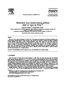
Finally, we have applied EMA18on to the determination of the performance of the known methods. It is clear that EMA18on, which is a fast and simple method, can be successfully applied to the decision-making problems in various areas such as machine learning and image enhancement. Although we have no proof about the accuracy of the results of such methods, the results are in compliance with our observations. In order to help in checking the accuracy of the comparison made by a soft decision-making method, we give, in Fig. 13-16, the Cameraman image with different SPN ratios and show the denoised images via the above-mentioned filters. It must be noted that these images has no information of their running times. Whereas, the use of a filter in a software depends on its running time is short. In other words, the running time of a filter is so significant that it can not be ignored. As a result, it is understood that f pf smatrices are an effective mathematical tool to deal with the situations in which more than one parameter or objects are used.
99
Journal of New Theory 25 (2018) 84-102
(a)
(b)
(c)
(d)
Fig. 13. (a) Original image “Cameraman” (b) Noisy image with SPN ratio of 10%, (c) Noisy image with SPN ratio of 50%, and (d) Noisy image with SPN ratio of 90%
(a) DBA
(b) MDBUTMF
(c) NAFSM
(d) DAMF
(e) AWMF
Fig. 14. The images having with SPN ratio of 10% before denoising.
(a) DBA
(b) MDBUTMF
(c) NAFSM
(d) DAMF
(e) AWMF
Fig. 15. The images having with SPN ratio of 50% before denoising.
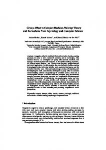
(a) DBA
(b) MDBUTMF
(c) NAFSM
(d) DAMF
(e) AWMF
Fig. 16. The images having with SPN ratio of 90% before denoising. Acknowledgements We thank Dr. U˘gur Erkan for technical support. This work was supported by the Office of Scientific Research Projects Coordination at C ¸ anakkale Onsekiz Mart University, Grant number: FBA-2018-1367.
Journal of New Theory 25 (2018) 84-102
100
References [1] D. Molodtsov, Soft set theory-first results, Computers and Mathematics with Applications 37 (1999) 19–31. [2] P. K. Maji, R. Biswas, A. R. Roy, Fuzzy soft sets, The Journal of Fuzzy Mathematics 9 (3) (2001) 589–602. [3] P. K. Maji, A. R. Roy, R. Biswas, An application of soft sets in a decision making problem, Computers and Mathematics with Applications 44 (2002) 1077–1083. [4] P. K. Maji, R. Biswas, A. R. Roy, Soft set theory, Computers and Mathematics with Applications 45 (2003) 555–562. [5] N. C ¸ a˘gman, S. Engino˘glu, Soft set theory and uni-int decision making, European Journal of Operational Research 207 (2010) 848–855. [6] N. C ¸ a˘gman, S. Engino˘glu, Soft matrix theory and its decision making, Computers and Mathematics with Applications 59 (2010) 3308–3314. [7] N. C ¸ a˘gman, F. C ¸ ıtak, S. Engino˘glu, Fuzzy parameterized fuzzy soft set theory and its applications, Turkish Journal of Fuzzy Systems 1 (1) (2010) 21–35. [8] N. C ¸ a˘gman, S. Engino˘glu, F. C ¸ ıtak, Fuzzy soft set theory and its applications, Iranian Journal of Fuzzy Systems 8 (3) (2011) 137–147. [9] N. C ¸ a˘gman, F. C ¸ ıtak, S. Engino˘glu, FP-soft set theory and its applications, Annals of Fuzzy Mathematics and Informatics 2 (2) (2011) 219–226. [10] N. C ¸ a˘gman, S. Engino˘glu, Fuzzy soft matrix theory and its application in decision making, Iranian Journal of Fuzzy Systems 9 (1) (2012) 109–119. [11] S. Engino˘glu, Soft matrices, PhD dissertation, Gaziosmanpa¸sa University (2012). ˙ Zorlutuna, On topological structures of fuzzy parametrized soft [12] S. Atmaca, I. sets, The Scientific World Journal 2014 (2014) Article ID 164176, 8 pages. [13] S. Engino˘glu, N. C ¸ a˘gman, S. Karata¸s, T. Aydın, On soft topology, El-Cezerˆı Journal of Science and Engineering 2 (3) (2015) 23–38. [14] F. C ¸ ıtak, N. C ¸ a˘gman, Soft int-rings and its algebraic applications, Journal of Intelligent and Fuzzy Systems 28 (2015) 1225–1233. [15] M. Tun¸cay, A. Sezgin, Soft union ring and its applications to ring theory, International Journal of Computer Applications 151 (9) (2016) 7–13. [16] F. Karaaslan, Soft classes and soft rough classes with applications in decision making, Mathematical Problems in Engineering 2016 (2016) Article ID 1584528, 11 pages. ˙ Zorlutuna, S. Atmaca, Fuzzy parametrized fuzzy soft topology, New Trends [17] I. in Mathematical Sciences 4 (1) (2016) 142–152.
Journal of New Theory 25 (2018) 84-102
101
[18] A. Sezgin, A new approach to semigroup theory I: Soft union semigroups, ideals and bi-ideals, Algebra Letters 2016 (3). [19] E. Mu¸stuo˘glu, A. Sezgin, Z. K. T¨ urk, Some characterizations on soft uni-groups and normal soft uni-groups, International Journal of Computer Applications 155 (10) (2016) 8 pages. [20] S. Atmaca, Relationship between fuzzy soft topological spaces and (X, τe ) parameter spaces, Cumhuriyet Science Journal 38 (2017) 77–85. [21] S. Bera, S. K. Roy, F. Karaaslan, N. C ¸ a˘gman, Soft congruence relation over lattice, Hacettepe Journal of Mathematics and Statistics 46 (6) (2017) 1035– 1042. [22] F. C ¸ ıtak, N. C ¸ a˘gman, Soft k-int-ideals of semirings and its algebraic structures, Annals of Fuzzy Mathematics and Informatics 13 (4) (2017) 531–538. [23] A. Ullah, F. Karaaslan, I. Ahmad, Soft uni-Abel-Grassmann’s groups, European Journal of Pure and Applied Mathematics 11 (2) (2018) 517–536. [24] A. Sezgin, N. C ¸ a˘gman, F. C ¸ ıtak, α-inclusions applied to group theory via soft set and logic, Communications Faculty of Sciences University of Ankara Series A1 Mathematics and Statistics 68 (1) (2019) 334–352. [25] S. A. Razak, D. Mohamad, A soft set based group decision making method with criteria weight, World Academy of Science, Engineering and Technology 5 (10) (2011) 1641–1646. [26] S. Eraslan, A decision making method via topsis on soft sets, Journal of New Results in Science (8) (2015) 57–71. [27] S. A. Razak, D. Mohamad, A decision making method using fuzzy soft sets, Malaysian Journal of Fundamental and Applied Sciences 9 (2) (2013) 99–104. [28] P. K. Das, R. Borgohain, An application of fuzzy soft set in multicriteria decision making problem, International Journal of Computer Applications 38 (12) (2012) 33–37. [29] S. Eraslan, F. Karaaslan, A group decision making method based on topsis under fuzzy soft environment, Journal of New Theory (3) (2015) 30–40. ˙ Deli, Means of fp-soft sets and their applications, Hacettepe [30] N. C ¸ a˘gman, I. Journal of Mathematics and Statistics 41 (5) (2012) 615–625. [31] K. Zhu, J. Zhan, Fuzzy parameterized fuzzy soft sets and decision making, International Journal of Machine Learning and Cybernetics 7 (2016) 1207–1212. [32] S. Vijayabalaji, A. Ramesh, A new decision making theory in soft matrices, International Journal of Pure and Applied Mathematics 86 (6) (2013) 927–939.
Journal of New Theory 25 (2018) 84-102
102
[33] N. Khan, F. H. Khan, G. S. Thakur, Weighted fuzzy soft matrix theory and its decision making, International Journal of Advances in Computer Science and Technology 2 (10) (2013) 214–218. [34] S. Engino˘glu, S. Memi¸s, A configuration of some soft decision-making algorithms via f pf s-matrices, Cumhuriyet Science Journal 39 (4) (2018) In Press. [35] S. Engino˘glu, S. Memi¸s, B. Arslan, A fast and simple soft decision-making algorithm: EMA18an, International Conference on Mathematical Studies and Applications, Karaman, Turkey, 2018. [36] A. Pattnaik, S. Agarwal, S. Chand, A new and efficient method for removal of high density salt and pepper noise through cascade decision based filtering algorithm, Procedia Technology 6 (2012) 108–117. [37] S. Esakkirajan, T. Veerakumar, A. Subramanyam, C. PremChand, Removal of high density salt and pepper noise through modified decision based unsymmetric trimmed median filter, IEEE Signal Processing Letters 18 (5) (2011) 287–290. [38] K. Toh, N. Isa, Noise adaptive fuzzy switching median filter for salt-and-pepper noise reduction, IEEE Signal Processing Letters 17 (3) (2010) 281–284. [39] U. Erkan, L. G¨okrem, S. Engino˘glu, Different applied median filter in salt and pepper noise, Computers and Electrical Engineering 70 (2018) 789–798. [40] Z. Tang, K. Yang, K. Liu, Z. Pei, A new adaptive weighted mean filter for removing high density impulse noise, in: Eighth International Conference on Digital Image Processing (ICDIP 2016), Vol. 10033, International Society for Optics and Photonics, 2016, pp. 1003353/1–5. [41] Z. Wang, A. Bovik, H. Sheikh, E. Simoncelli, Image quality assessment: From error visibility to structural similarity, IEEE Transactions on Image Processing 13 (4) (2004) 600–612.