On Spectrum Probing in Cognitive Radio Networks - IEEE Xplore

This full text paper was peer reviewed at the direction of IEEE Communications Society subject matter experts for publication in the IEEE ICC 2010 proceedings

On Spectrum Probing in Cognitive Radio Networks: Does Randomization Matter? Chao Chen, Zesheng Chen, Todor Cooklev, and Carlos Pomalaza-R´aez Indiana University - Purdue University Fort Wayne, Indiana 46805 Abstract—In cognitive radio networks, dynamic spectrum access is achieved by allowing secondary users (SUs) to probe the spectrum and utilize available channels opportunistically. Spectrum probing mechanisms should be efficient and fast to avoid harmful interference with primary users (PUs). Periodic probing has been commonly adopted as a default spectrum probing mechanism. In this paper, we attempt to study different spectrum probing mechanisms and evaluate a performance metric called the probing delay, i.e., how quickly a probing mechanism can detect a channel change. We find that randomization in the probing strategy does affect the probing delay. Specifically, in the independent sensing scenario, periodic probing indeed achieves the smallest probing delay. In the cooperative sensing scenario, however, randomization can drastically reduce the probing delay.

I. I NTRODUCTION Dynamic spectrum access techniques have been proposed to address the spectrum inefficiency problem inherent in current static channel allocation policies. In cognitive radio networks (CRNs), secondary users (SUs) or unlicensed users are allowed to access licensed spectrum channels opportunistically without harmful interference with primary users (PUs) or licensed users. To achieve this goal, SUs must be equipped with cognitive radios that can monitor the channel usage and determine whether the PUs are present. Spectrum sensing is critical to the design of cognitive radio networks to achieve a balance between providing efficient reuse of spectrum and protecting PUs against interference from SUs. For such a purpose, FCC has set a strict guideline on spectrum sensing. For example, in IEEE 802.22 [1], the first international standard for wireless regional area networks using cognitive radio techniques, PUs should be detected within 2 seconds of their appearance with the probability of misdetection (PM D ) and the probability of false detection (PF A ) less than 0.1. To meet these requirements, spectrum sensing techniques need to be both accurate and fast. The performance of spectrum sensing in a CRN depends not only on the detection method that is affected by the physical and MAC layer features of PUs, but also on the channel scan strategies of SUs and how SUs cooperate in sensing [2], [3]. Meanwhile, the SUs’ power and control overhead associated with spectrum sensing should be taken into consideration. In this paper, we investigate the delay performance of spectrum sensing. Note that we are not interested in the specific underlying physical and MAC techniques that detect channel opportunities. Instead, we focus on how SUs in a CRN effectively schedule their channel scans and how different scan

scheduling strategies would affect the speed of detecting the PU signals. We use the term “spectrum probing” in this paper to specifically refer to such scheduling policies and avoid confusion with the more general term “spectrum sensing.” One of the main purposes of spectrum probing is to detect the absence and the return of PU signals in a channel in a timely manner, so that the SUs can utilize licensed spectrum bands opportunistically without interrupting the PUs. Most existing works either do not specify the spectrum probing scheme or just assume periodic channel scanning for spectrum probing [4]–[6]. That is, SUs probe channels periodically to detect the absence of PU signals. Once a channel is found to be available, SUs can utilize the channel opportunistically. Meanwhile, when SUs are using the available channels, they also keep probing these channels periodically to detect the PUs’ return and thus exit the channels. The reason for choosing such a periodic spectrum probing mechanism, however, is not clear other than its simplicity. When a cognitive radio network has multiple SUs, all SUs can collaborate in sensing a channel to enhance the detection of PU signals to get higher sensing quality and faster PU signal detection. Several cooperative sensing mechanisms have been proposed to overcome uncertainties under channel randomness such as fading/shadowing [7]–[10]. A SU shares the sensing result with other SUs to determine the presence of PUs. Existing cooperative sensing schemes, however, consider that all SUs are synchronized in sensing the channel. That is, all SUs probe the channel at the same time. No research has been done to evaluate the delay performance of such a synchronized probing mechanism and to study other possible ways to coordinate SUs probing schedules. In this research, we consider the randomization in spectrum probing mechanisms and study their delay performance using the renewal theory and the stochastic ordering concept. Specifically, we evaluate a performance metric called the probing delay, i.e., how quickly a probing mechanism can detect a channel change. Our work makes the following contributions: • We study the probing delay of spectrum probing mechanisms both under the independent sensing scenario where SUs make independent decisions and the cooperative sensing scenario where SUs collaborate in determining the spectrum usage. Besides the classical periodic probing, probing mechanisms with certain levels of randomization (e.g., with some flexibility on how SUs initiate channel scans and how the probing interval is distributed) are also considered (See Fig. 1).

978-1-4244-6404-3/10/$26.00 ©2010 IEEE


Under the independent sensing scenario, we find that with the same power budget on spectrum probing, periodic probing always yields the minimum probing delay, even if the detection method is not 100% accurate. • Under the cooperative sensing scenario, if SUs add randomization into the spectrum probing mechanism, the probing delay can be reduced significantly compared with the synchronized periodic probing. The improvement in probing delay grows if more SUs in a CRN cooperate in sensing the spectrum. The remainder of this paper is structured as follows. Section II introduces the system model, problem definition, and our approach. Section III and Section IV study the probing delay of spectrum probing mechanisms under the independent sensing scenario and the cooperative sensing scenario, respectively. Section V evaluates the delay performance through simulations. Finally, Section VI concludes this paper. •

II. P ROBLEM S ETUP A. System Model A CRN with a group of SUs is considered. The SUs monitor licensed channels for possible spectrum opportunities. Similar to the channel-usage model in [6], a channel is modeled as a renewal process alternating between ON and OFF states. A channel is in ON (or OFF) state, if a PU signal is present (or absent). The sojourn times of ON and OFF states of a channel are represented by two random variables TON and TOF F that are independent of each other. Each SU can be dynamically reconfigured as a transceiver or a sensor. When used as a spectrum sensor, a SU monitors a channel to detect PU signals and thus determine whether the channel is available for use by SUs. Once SUs utilize a licensed channel that has been discovered to be idle, the SUs keep monitoring the channel so that upon the PUs’ return, the channel can be vacated promptly. We assume that a SU detects the presence (or absence) of PU signals during a certain time period, called the “probing time” Tp . The probing time is determined by the underlying detection method and the features of PU signals. It is assumed that the status of a channel remains unchanged during the probing time. That is, Tp is small compared with E[TON ] and E[TOF F ]. B. Problem Definition We investigate the probing delay of spectrum probing mechanisms. Here the “probing delay” is defined as the time from a change of channel status (i.e., from ON to OFF or from OFF to ON) to the detection of such a change by a CRN. Specifically, we study the following problems: 1) What is the probing delay if SUs chooses the periodic channel scan strategy for spectrum probing? 2) Under the condition that SUs spend the same amount of power in spectrum probing, can periodic probing detect a channel change with a smaller probing delay than other probing schemes with randomization? 3) If SUs cooperate in detecting the channel usage, how would the probing delay be affected?

Fig. 1.

Illustration of spectrum probing mechanisms.

C. Our Approach As illustrated in Fig. 1, a SU probes a channel that alternates between ON and OFF states. We use Xi to denote the time interval between the SU’s ith and (i + 1)th channel scan (i = 1, 2, ...). A SU can choose periodic probing to scan the channel so that all Xi ’s are equal and fixed, i.e., Xi = μ. Alternatively, a SU can utilize a spectrum probing mechanism with some randomization, i.e., Xi ’s are independent and identically distributed (i.i.d.) random variables with a distribution function FX (t). In this paper, we use D to denote the expected value of the probing delay. To compare the average probing delay of periodic probing with those of different random probing mechanisms, we assume that the average amount of power that a SU spends in sensing the channel is fixed, i.e., the average probing interval E[X] is fixed and takes a constant value μ. Common examples of random probing mechanisms include uniform probing and Poisson probing. For uniform probing, the probe interval X follows a uniform distribution within [0, 2μ], i.e., ⎧ if t ≤ 0 ⎨ 0, t , if 0 < t ≤ 2μ (1) FX (t) = ⎩ 2µ 1, otherwise. For Poisson probing, the probe interval X follows an exponential distribution with mean μ, i.e., 0, if t ≤ 0 FX (t) = (2) 1 − e−t/µ , if t > 0. In this paper, we consider two scenarios based on whether the SUs collaborate in channel detection. In the first scenario, all SUs in a CRN make their own decisions about the channel status independently from other SUs. In the second scenario, SUs collaborate in sensing a channel change. A simple OR rule [11] is adopted to determine the channel status: All SUs independently probe the same channel, and as soon as one SU senses a change in the channel status, it will inform all other SUs about the change. For simplicity, we do not consider any specific cooperative schemes on how SUs share their detection results. Instead, we assume that this sharing of information can be done in a considerably small amount of time. In the following two sections, we analyze the average probing delay D of different spectrum probing mechanisms under these two scenarios.


m delay for this channel change is D(t) = Y (t) + i=1 Xi with a probability (1 − p)m p. Therefore,

+∞ m m (1 − p) p Y (t) + Xi . (4) E[D(t)|Xi , Y (t)] = m=0

Fig. 2.

Probing delay under uncertain detection.

III. I NDEPENDENT S ENSING In the independent sensing scenario, all SUs monitor the channel and make their own decisions about the channel status. Therefore, we study a simple case that a SU monitors one channel and study the average probing delay of this SU. In this section, we consider two cases where SUs always detect the channel status correctly and SUs detect the channel status with some error probability. A. Case 1: Perfect Detection If a SU always correctly determines the channel status in the probing time Tp . Let {N (t), t ≥ 0} be the number of scans occurred before time t. Since the time intervals between two successive probes (Xi ’s) are i.i.d., N (t) can be regarded as a renewal process. We further define Y (t) as the residual time from t until the next scan. Since a change in the channel status can occur at any time t, the average probing delay D is equal to the expected value of Y (t), which can be calculated using the renewal reward theory [12] as: s Y (t)dt D = E[Y ] = lim 0 s→+∞ s X E[ 0 (X − t)dt] E[reward during a cycle] (3) = = E[length of a cycle] E[X] var[X] + E 2 [X] var[X] μ E[X 2 ] = = + . = 2E[X] 2E[X] 2μ 2 Here, X is the probing interval. Since var[X] ≥ 0, D ≥ µ2 , where the equality holds when var[X] = 0, which means that Xi ’s are all equal. The above formula states that if the average probing interval μ is given, when a SU uses periodic probing, a minimum average probing delay can be achieved, which is half the probing interval. If a SU chooses a random probing mechanism, var[X] is positive. Therefore, the average probing delay is always larger than µ2 . For example, for uniform probing with mean μ, var[X] = μ2 /3, and D = 23 μ; for Poisson probing, var[X] = μ2 , and D = μ. B. Case 2: Detection with Uncertainty A SU may not always detect the channel status successfully in the probing time Tp . For example, a SU may detect the appearance of PUs with a probability of misdetection (PM D ) and a probability of false detection (PF A ). Here we assume that PM D = PF A = 1 − p, where 0 ≤ p ≤ 1. As shown in Fig. 2, if a SU detects a channel status change at t after m (m = 0, 1, 2, ...) continuous unsuccessful scans, the probing

i=1

Since Xi ’s are i.i.d., E[Xi ] = E[X], the average probing delay D can be calculated as follows: D = E[D(t)] = E[E[D(t)|Xi , Y (t)]] +∞ (1 − p)m p(E[Y ] + mE[X]) = m=0

= E[Y ] +

+∞

m

m(1 − p) p

· E[X]

(5)

m=1

1−p ·μ p 1 1−p var[X] + + · μ, = 2μ 2 p

= E[Y ] +

by applying (3). When Xi ’s are all equal, var[X] = 0, D 1−p 1 achieves the minimum value 2 + p μ. The above formula states that when a SU senses the spectrum with a fixed average probing interval and a successful detection

probability μ of p, a minimum average probing delay of 12 + 1−p p can be achieved if periodic probing is used. In comparison, random spectrum probing mechanisms always generate a longer average probing delay. For example, for uniform μ; for Poisson probing, probing with mean μ, D = 23 + 1−p p

1−p D = 1 + p μ. Furthermore, D decreases as p grows larger. As a special case, when p = 1, i.e., all channel scans are successful, the above formula reduces to (3). In summary, when SUs sense the channel independently (i.e., SUs do not cooperate and make detection decisions only based on local information), periodic probing always yields the fastest average probing delay among all possible spectrum probing mechanisms. IV. C OOPERATIVE S ENSING In the cooperative sensing scenario, we choose the OR rule that the probing delay of a CRN is determined by the SU that first senses a channel status change. Therefore, the average probe delay D of the CRN is the expected time from a channel status change till the first SU detects such a change. We define Yi (t) as the residual time from t until the next scan from the ith SU. Then the residual time Y (t) from t until the next probe from any SU in the CRN is Y (t) = mini Yi (t). Suppose that SUs can probe the channel with some randomness, i.e., each SU can probe the channel at random times independently from others. We consider the following two variations of periodic probing, based on the level of coordination among SUs: • Synchronized periodic probing: All SUs initiate spectrum probing at the same time, so that the probing events of all SUs are aligned in time. This is the scheme that is


adopted by most current cooperative spectrum probing mechanisms. • Independent periodic probing: Each SU independently initiates channel scans while keeping the probing interval fixed. For random probing, different SUs can choose different distribution functions for the probing interval X, for example, uniform distribution and exponential distribution. Meanwhile, each SU initiates channel scans independently from other SUs. For all the above cases, we assume that all SUs spend the same average amount of power in sensing the channel, i.e., the average probe interval of all SUs is the same (E[X] = μ). For the simplicity of analysis, we study the case when p = 1, i.e., all channel scans are successful and yield 100% detection probability in the probing time Tp . For the cases of uncertain detection, we will use simulations to evaluate the probing delay performance in Section V. A. Periodic Probing If all SUs always correctly determine the channel status in the probing time Tp , the average probe delay D = E[Y ]. 1) Synchronized Periodic Probing: Under perfect detection, if the probing events of all SUs are synchronized, the delay performance is equivalent to having a single SU probing the channel. According to (3), the probing delay D = µ2 . 2) Independent Periodic Probing: In this case, since all SUs independently initiates their channel scans, Yi ’s are independent. Therefore, from the order statistics [12], P (Y > t) = P (min Yi > t) i

= P (Y1 > t, Y2 > t, ..., YN > t) =

N

(6)

N

P (Yi > t) = [1 − FYi (t)] .

i=1

The average probing delay can be calculated by +∞ +∞ D = E[Y ] = F (Y > t)dt = [1 − FYi (t)]N dt. 0

0

(7) As the time interval between two successive probes is fixed at μ for periodic probing, we consider that a SU starts its first channel scan with an offset within [0, μ] from time 0. If such an offset is uniformly distributed within [0, μ], the cumulative distribution function of Y is ⎧ if t ≤ 0 ⎨ 0, t/μ, if 0 < t ≤ μ (8) FYi (t) = ⎩ 1, otherwise. According to (7), the average probing delay is µ D= (1 − t/μ)N dt.

(9)

0

Setting x = t/μ, D=

0

1

(1 − x)N μdx =

μ . N +1

(10)

As shown above, under the perfect detection condition, if all SUs choose periodic probing, letting SUs starts their channel scans independently from others will yield an average probing delay that is only N2+1 of the probing delay in the case of synchronized periodic probing. If N is large, this reduction in probing delay will be significant. As a special case of periodic probing, if channel scans of all SUs are evenly distributed in a probe interval, a smaller probing delay can be achieved. Specifically, for a CRN with N SUs, if the first SU initiates spectrum probing at time t0 , then the ith SU will start probing the channel at time t0 + i−1 N μ, i = 1, 2, ..., N . Under perfect detection, this case is equivalent to a single SU system where the SU senses the µ . Therespectrum periodically using a probing interval of N µ , fore, according to (3), the average probing delay D = 2N which is even smaller than the case of independent periodic probing. To achieve the performance gain, however, all SUs need to be controlled in a highly coordinated manner: Starting their channel scans in turn and these scans are equally spaced within a probing interval μ. This requires a central server and a dedicated control channel to coordinate the channel scans of all SUs, which adds to the system complexity. Moreover, the central server needs to know N ahead of time. If a CRN allows SUs to dynamically join and leave the network, such coordination would be very difficult to implement. Thus, we do not include this special case of periodic probing for further comparison with other spectrum probing mechanisms. B. Random Probing For random probing, different SUs initiate their channel scans independently. Therefore, (6) still holds. 1) Poisson Probing: If the distribution of the probing interval X is exponential with mean μ, because of the memoryless property of the exponential distribution, the residual time Yi (t) from any time t until the next scan is also exponential with the same mean. Therefore, FYi (t) = 1 − e−t/µ , t > 0. According to (7), the average probing delay can be calculated as: +∞ μ (11) e−N t/µ dt = . D= N 0 2) General Distribution of the Probing Interval: For a general distribution of the probing interval X, the residual time Yi usually does not have the same distribution as X. According to the renewal theorem [12], the cumulative distribution function of Yi can be derived from the distribution of X: t (1 − FX (τ ))dτ 0 . (12) FYi (t) = +∞ (1 − FX (τ ))dτ 0 Then we can plug FYi (t) into (7) to calculate the average probing delay D. Let’s take uniform probing as an example. If the probing interval of all SUs follows a uniform distribution within [0, 2μ] with mean μ, plugging (1) into (12), we can get ⎧ if t ≤ 0 ⎨ 0, t t2 (13) FYi (t) = − , if 0 < t ≤ 2μ ⎩ µ 4µ2 1, otherwise.


12

12 Simulation Analysis

Simulation Analysis

8

6

4

2

10 Probing delay (seconds)


Probing delay (seconds)

10

8

6

4

2

0 0

12 Simulation Analysis

2 3 4 Average probing interval (seconds)

5

(a) Periodic probing. Fig. 3.

0

6

4

2

0 1

8

0 1


5

0

(b) Uniform probing.

1


5

(c) Poisson probing.

Average probing delay of spectrum probing mechanisms under the independent sensing scenario (perfect detection).

According to (7), N t2 t 1− + 2 D= dt μ 4μ 0 2µ 2N t = 1− dt. 2μ 0

2.5

2µ

(14)

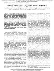
Following the same procedure as in (10), we can get D = 2µ 2N +1 for the case of uniform probing. In summary, when cooperative sensing is considered, instead of using synchronized periodic probing, if SUs add randomization by letting SUs initiates channel scans independently or choose a random distribution for the probing interval, the average probing delay D can be decreased. The improvement in probing delay grows as the number of SUs N increases. Moreover, the randomization also releases the burden of CRNs to synchronize the channel scans of all SUs. Hence, the related control overhead can be reduced as well. V. S IMULATION R ESULTS In this section, we use computer simulations to evaluate the delay performance of spectrum probing mechanisms and verify the analytical results. Specifically, three probing mechanisms are simulated: periodic probing, uniform probing, and Poisson probing. In a simulation run, a channel change (either from ON to OFF or from OFF to ON) occurs at a random time t0 within a duration of length 104 ×μ. In the independent sensing scenario, one SU senses the channel with a specific probing mechanism. Once the SU detects the channel change successfully at time t1 , we record the probing delay t1 − t0 . In the cooperative sensing scenario, multiple SUs sense the channel, t1 is the time that the first SU successfully detects the channel change. For each set of simulation, we carry out 104 independent runs and calculate the average probing delay D and its variation. We first evaluate the average probing delay of the three spectrum probing mechanisms with different average probing intervals under the independent sensing scenario. Under perfect detection, as shown in Fig. 3, the simulation results overlap with the analysis results for each probing mechanism.


1.5

1

0.5

0 0.8

Simulation (Periodic) Analysis (Periodic) Simulation (Uniform) Analysis (Uniform) Simulation (Poisson) Analysis (Poisson) 0.85

0.9 Detection probability

0.95

1

Fig. 4. Average probing delay of spectrum probing mechanisms under the independent sensing scenario (detection with uncertainty): µ = 2 seconds.

The error bar in Fig. 3 represents the standard deviation of the probing delay in 104 runs. Compared with uniform probing and Poisson probing, periodic probing always produces a smaller probing delay with a smaller variation. Fig. 4 depicts the probing delay when the detection probability p varies from 0.8 to 1. In this case, we fix the average probing interval at 2 seconds. We can see that periodic probing still gives a smaller probing delay than the two random probing mechanisms. The probing delay improvement of periodic probing is as large as 17% and 40% compared with those of uniform probing and Poisson probing, respectively, when p = 0.8. As p grows, the improvement in the probing delay is even greater. In the cooperative sensing scenario, we fix the average probing interval to 2 seconds and evaluate the probing delay under different spectrum probing mechanisms. The periodic probing we simulated in this scenario is the independent periodic probing scheme. Fig. 5 shows the probing delay when the number of SUs in a CRN changes from 1 to 30. For reference, in each of the three subfigures, the horizontal line (D = 1 second) represents the probing delay of the synchronized periodic probing. We can see that with some


Simulation Analysis

Simulation Analysis

3

2

1

0

3

2

1

0

0

5

10 15 20 Number of secondary users

25

30

0

5


(b) Uniform probing.


1

25

30

0

5


25

30

(c) Poisson probing.

VI. C ONCLUSIONS

0.12

0.115

0.11

0.105

0.1

0.09 0.8

2

Average probing delay of spectrum probing mechanisms under the cooperative sensing scenario (perfect detection): µ = 2 seconds.

0.125

0.095

3

0

(a) Independent periodic probing. Fig. 5.

Simulation Analysis

4


4



4

Simulation (Independent periodic) Simulation (Uniform) Simulation (Poisson) 0.85

0.9 Detection probability

0.95

1

Fig. 6. Average probing delay of spectrum probing mechanisms under the cooperative sensing scenario (detection with uncertainty): µ = 2 seconds, N = 20.

randomization, all these three spectrum probing mechanisms can generate a probing delay no greater than 1 when N > 1. The improvement in probing delay is more significant when N grows larger. Moveover, when N is small, compared with the case of independent periodic probing, the probing delays of uniform probing and Poisson probing have both larger values and larger variations. When N is larger, however, such differences become less evident. Next, we compare the probing delay of spectrum probing mechanisms when the detection probability p varies between 0.8 and 1. In this case, the average probing interval is fixed at 2 sec and the number of SUs in a CRN is fixed at 20. The simulation results are given in Fig. 6. We can see that among the three spectrum probing mechanisms with randomization, independent periodic probing gives a shorter probing delay than the other two random probing schemes. Nevertheless, all these three produce much smaller probing delays than that of synchronized periodic probing (which is 1.5 seconds when p = 0.8 and 1 second when p = 1).

In this paper, we study the delay performance of various spectrum probing mechanisms. We find that under the same power budget on spectrum probing, periodic probing allows a single SU to detect the channel change with the minimum delay. If SUs in a CRN collaborate in detecting the channel change, probing mechanisms with some randomization can reduce the probing delay, especially when the number of SUs is large. Moreover, such randomization does not add to extra power consumption or system design complexity. For future work, we plan to study the delay performance of spectrum probing mechanisms when SUs have some knowledge about the traffic patterns of PUs. R EFERENCES [1] IEEE 802.22, Working Group on Wireless Regional Area Networks, http://www.ieee802.org/22/. [2] I. F. Akyildiz, W.-Y. Lee, M. C. Vuran, and S. Mohanty, “NeXt generation/dynamic spectrum access/cognitive radio wireless networks: a survey,” Computer Networks, vol. 50, no. 13, pp. 2127-2159, Sept. 2006. [3] T. Yucek and H. Arslan, “A survey of spectrum sensing algorithms for cognitive radio applications,” IEEE Communications Surveys and Tutorials, vol. 11, no. 1, pp. 116-130, 2009. [4] N. Chang and M. Liu, “Optimal channel probing and transmission scheduling for opportunistic spectrum access,” in Proc. ACM MobiCom 2007, pp. 27-38. [5] H. Kim and K. G. Shin, “Fast discovery of spectrum opportunities in cognitive radio networks,” in Proc. of IEEE DySPAN 2008. [6] H. Kim and K. G. Shin, “Efficient discovery of spectrum opportunities with MAC-layer sensing in cognitive radio networks,” IEEE Transaction on Mobile Computing, vol. 7, no. 5, pp. 533-545, May 2008. [7] A. Ghasemi and E. S. Sousa, “Collaborative spectrum sensing for opportunistic access in fading environments,” in Proc. of IEEE DySPAN 2005, pp. 131-136. [8] G. Ganesan and Y. Li, “Cooperative spectrum sensing in cognitive radio networks,” in Proc. of IEEE DySPAN 2005, pp. 137-143. [9] S. M. Mishra, A. Sahai, and R. W. Brodersen, “Cooperative sensing among cognitive radios,” in Proc. of IEEE ICC 2006, pp. 1658-1663. [10] J. Unnikrishnan and V. V. Veeravalli, “Cooperative sensing for primary detection in cognitive radio,” IEEE Journal of Selected Topics in Signal Processing, vol. 2, no. 1, pp. 18-27, Feb. 2008. [11] E. Peh and Y.-C. Liang, “Optimization for Cooperative Sensing in Cognitive Radio Networks,” in Proc. of IEEE WCNC 2007, pp. 27-32. [12] S. Ross, “Introduction to Probability Models,” eighth edition, Academic Press.