Pmceedings of the 40th lEEE Conrerenee on Decision and Control Orlando, Florida USA, Doeember 2001
TuA05-4
On Stabilization of Nonlinear Distributed Parameter Port-Controlled Hamiltonian Systems via Energy-Shaping’ Hugo Rodriguez’, Arjan J. van der Schaft* and Romeo Ortega’ “Laboratoire des Signaux et Systemes, Supelec ‘Department of Signals, Systems and Control Plateau de Moulon Faculty of Mathematical Sciences University of Twente, The Netherlands 91192 Gif-sur-Yvette, France Email: {cortes}
[email protected] Email: a.j.vanderschaft0math.utwente.nl Phone: +33 1 69851766, FAX: +33 1 69851765 Phone: +31 53 4893370, FAX +31 53 4340733
Abstract Energy-shaping techniques have been successf~lly used for stabilization of nonlinear finite dimensional systems for 20 years now. In particular, for systems described by Port-Controlled Hamiltonian (PCH) models, the “control by interconnection” method provides a simple and elegant procedure for stahilization of nonlinear systems with finite dissipation. In this paper we explore the possibility of extending this technique to the case where the plant contains a distributed parameter subsystem, in the form of a transmission line between the plant and the controller. Note: The present paper is an abridged version of I31
Instrumental for our developments is the notion of a Dirac structure, that formalizes in a geometric language the concept of power conserving interconnection for PCH systems. Dirac structures for finite dimensional implicit PCH systems are reported in [4]. Recently, the framework was extended to distributed parameter systems in [GI. The main contribution of this paper is the derivation of the conditions for existence of the Casimir functions for a controller-infinite dimensional subsystem-plant configuration. In the next section we present the Dirac structure associated to PCH models, for reference we start with finite dimensional systems, and then present the infinite dimensional case. Section 4 contains our main result, first, we present the interconnection between lumped and distributed parameter systems described above. Then, we find the conditions that guarantee the existence of Casimir functions for the interconnected system. Finally, we outline an stabilization procedure for the interconnected PCH system based in the results of 15, 91 and we present a controller design example, and then wrap up the paper with some concluding remarks in Section 5.
1 Introduction Passivity-based control (PBC) of finite dimensional systems was introduced already 20 years ago, and has reached a good level of maturity with many different variations and successful applications, see e.g. [4, 1, 21 for a list of references. The basic underlying principles of PBC is to shape the total energy of the system, which is clearly independent of the dimension of the state space. Hence, it seems natural to look for possible extensions of PBC to the distributed setting; this is the topic that we address in the present paper. The PBC design technique that we consider here is the “control by interconnection” method developed for regulation of Port-Controlled Hamiltonian (PCH) systems’ in 121, see also Section 4.3.1 of 141. As thoroughly detailed in the aforementioned refeiences, and
2 D i r a c Structures and Port Controlled H a m i l t o n i a n Systems It has been shown in [4, G] that the notion of power preserving interconnection can be formalized geometrically by a Dirac structure, which is a subspace of the In this section we briefly space Of efforts and present this concept for lumped systems as well as
‘This work has been partially supported .by the CONACyT of Mexico ‘PCH Systems are a natural extension of classical Hamiltonian systems to consider the existence of external variables, see 141.
0-7803-7061-9/01/$10.00 0 2001 IEEE
briefly explained in Section 3 below, the central component of this approach is the generation of Casimir functions, which are dynamical invariants independent of the Hamiltonian function that allow us to achieve the energy shaping objective.
131
recover the classicalbenergy variables-statespace description of the PCH system we recall that in these variables the energy stored by the conservative elements is defined by the Hamiltonian function, H ( z ) : R" -+ R, in such a way that the increase of energy equals power, that is , P ( t ) = % H [ z ( t ) ] = ( % [ z ( t ) ]I k ( t ) ) , hence, the flow and effort variables of the energy-storing elements are given by4 fs = 4 and es = In this way, we get the well-known model of a PCH system
for distributed parameter systems with a single scalar spatial variable ranging in a segment [0,l].
2.1 Lumped Parameter Systems To define the notion of a Dirac structure for lumped parameter systems we consider the finite dimensional linear space 7 of flows f , and its dual, +', which is the space of efforts e . Power is then defined as P = ( e I f ) with (.I.) denoting the duality product.' As shown in [4],on 7 x +* there exists a canonically defined symmetric bilinear form
< (fi,el),(fz,ez) & (el I f 2 ) + (e2 I f i )
E(.).
(2.1) which clearly satisfies the energy balance
Definition 1 A (constant) Dirac structure o n the f i nite dimensional linear space 7 is a linear subspace S c 3 x 7' such that SI = S, where SL denotes the orthogonal complement of S with respect to the bilinear f o r m (2.1).
in the following, we will use e p = yp and f p = up in order to relate to the standard input-output notation. 2.2 Distributed Parameter Systems In order to define the Dirac structure for such a distributed parameter system we have t o consider, instead of a finite-dimensional linear space 7 x +' as in the lumped parameter case, an infinite-dimensional function space; see [6]for a more general differentialgeometric setting appropriate t o multi-dimensional spatial domains.
As an immediate corollary of the definition we see that for all (f,e) E 'D we have that ( e ,f ) = 0. Hence, a Dirac structure defines a power conserving relation. Here, we are interested in PCH systems where the Dirac structure can be represented in input-output form as A
' D = { ( f , e ) ~ . ~ x Ixe *p = g T ( z ) e s , e R = g L ( z ) e S ,fS = - J ( Z ) e S - gR(Z).fR - g ( Z ) f p }
This function space 7 x 7' will be defined as follows. a Consider the function space C = ZIM(Z) x X I E ( Z )x B , with 'H1~(Z),'Hl~(Z) denoting the space of magnetic and electric efforts, e M and e E , respectively, and B denoting the external efforts e* a t the boundary of Z . Here X1(2) denotes the Sobolev space of .C2 functions on Z whose derivatives are also in Cz. Then .T is defined as the dual space of E with respect t o the duality ,product (defining again the power P )
(2.2) where := (fs, f ~ f,p , e s , e R , e p ) ', z E EX" is the systems state, J ( z ) = - J T ( z ) is the socalled interconnection matrix, and g(z), y~(.), Y R ( Z ) are input matrices of suitable dimensions. From (2.2) it is easy t o show that D = 'Dl. Furthermore, given that for all (f,e) E 'D = 'DL,we have 0 =< ( f , e ) , ( f , e ) >>= 2(f I e ) , therefore P = 0 for all elements of 'D, consequently, the Dirac structure defines a power conserving relation between the effort and flow variables. If we assume that the flow and effort variables of the dissipative elements are related by f R = - R ( Z ) e R , where R ( z ) = RT(Z) 2 0 , We obtain the following relationship between the power variables of the PCH system
((eE,eM>eb), ( f E >fM,fb))= Ji[fE(z)eE(z) f
fM(z)eM(z)ldr ebfb
16
with ( f ~f , ~fb) , denoting respectively the electric flow, the magnetic flow (both functions on Z be, the longing to the dual Sobolev space ' H l ( Z ) * ) and boundary flow. In analogy with (2.1), we can define a bilinear form between two elements of 7 x E as
~e >= ~ ehft + e L n ) d z + (
where R(z) := g R ( Z ) T R ( Z ) g R ( Z ) . w e call this the power variables representation of a PCH system. To 21f P is a Hilbert space, then 7 can be naturally identified with F in such a way that for all f E P , e E F* we have (e I f) = ( e ,f), where (.,.) is the standard inner product; see e.g. [8]. 3fs, fn. f p are the stored, the dissipated and the external flows respectively.
, ( e ~ f ~ + e ~ f ~ + (2.5) e + ~e ~ 16)
lStrictly speaking, the power variables fs,es do not live in a constant linear space but instead in the tangent and cwtangent spaces to the finite dimensional manifold of energy variables. This is formalized with the definition of a non-constant Dirac structure on a manifold, see [7] for details.
132
which satisfies the energy balancing equation
6;'fl(0)6~'fl(o) The proposition below, whose proof may he found in [3],defines the Dirac structure for the case of infinite dimensional systems with scalar spatial variables.
- s;'fl(e)a,'fl(e).
d?l dt
-
2.3 Example: Transmission L i n e In this subsection we present the PCH model of a transmission line whose dynamics are described by the well-known telegrapher's equations. In the Dirac framework the model is given as follows : The energy variables are electric charge and magnetic flux, qE(t) = q ( z , t ) , q M ( t ) = A(r,t), respectively. The total energy functional becomes 'fl = 2L f o[ &G ,q( Z dz. Then, the telegrapher's equations may be expressed as a distributed PCH system of the form (2.8), that is
P r o p o s i t i o n 1 Define the following subspace of 3 x
E
+a]
Then V is a constant Dirac structure, with respect to the bilinear form (2.5). We will now prove that, equivalently to the finite dimensional case, the elements of the Dirac structure of Proposition 1 satisfy a generalized form of power conservation. Indeed, from (2.5) we have that >= 0 , for all (f I e ) E V,that is, 0 , thus, We get 21; [eEfE + e ~ f ~ ] 4d Z 2ebfb e the energy balance property J", [eEfE eMfM] dr = eb(o)fb(o)-eb(e)fb(p),which Says that the total power in the domain Z is equal to the power ingoing a t the boundary 0 minus the power outgoing a t the bouudary e.
the lower relation of (2.9) defines voltages and currents a t the boundary points {0, !}. In the following we assume that the physical parameters of the transmission line are upper and lower bounded in [ O t ] , that is, Lm 5 5 LM, Cm 5 - CM with < L;,C; > 0, i = M , m.
&
+
3 Control by Interconnection : Finite Dimensional Case
The distributed parameter PCH system in power variables follows directly from the Dirac structure. Evaluating the lower relation of (2.6) a t the boundary points IO,[}, we get f o = -MO,
In this section we first briefly review the PBC design method of "control by interconnection" for lumped parameter systems, and then present its extension to the infinite dimensional case. A key step in this method, that allow us to achieve the energy shaping objective, is the generation of Casimir functions.
eo = eEo, fe = - e ~ e , ee = eEe (2.7)
In order to write (2.6) in energy variables, we consider the Hamiltonian density H : ' f l i l ~x* ' f l l ~ *x Z + LI,associated with the total energy functional 'fl = A J " i H ( g ) d z ,with Q = [ q ~ , q ~ , We r ] . assume 'fl to be differentiable, with time derivative [5]
E,
In the "control by interconnection" method we consider a PCH plant described by (2.4) in interconnection with a PCH controller with state z, E R", input U,, output yc, and H,(z,) the energy of the controller.' In power variables the PCH controller is described by
a
where we have introduced 6831 = 6 ~ ' f= l 6YE to denote the variational derivative. As in the lumped parameter case, the power and energy variables are a related by f~ = - $ Q E , f~ = - ~ Q M , eE = and ew = 6~31 and the distributed parameter PCH system (2.6) can be written in energy variables as
The interconnection constraints are power-preserving of the form U c = Yp, up = - y c (3.2) The composed system is clearly still Hamiltonian and can be written in power variables as
5See [4] for an explanation for the choice of this structure of the PCH controller.
133
--
a HCI(x) =
H(z)
+
3.1 Example: Control by Interconnection of RLC Circuit To illustrate the control by interconnection method let us consider a RLC circuit described by
Hc(z,)
the closedloop energy function (defined in an extended a state space = [ z , z , ] ~ ) We can easily see that this energy function is non-increasing, since $Hcl = -&% a= ( z ) R ( z ) % ( s5 ) 0, and we would like to shape it to assign a minimum at the desired point. However, although Hc(z,) can be freely assigned, the systems energy-function H ( z ) is given, and its not clear how can we effectively shape the overall energy. One possibility is to restrict the motion of the closed-loop system to a certain subspace of x, say R c Rn+m,by rendering R In this way, we can express the closed-loop total energy as a function of z only. In the Energy-Casimir method [2], we look for dynamical invariants which are independent of the Hamiltonian function. More precisely we look for functions C(x) -called Casimir functions- such that along the dynamics of the PCH system $C(x) = 0 independent of the energy function. Without loss of generality, we consider Casimir functions of the form C(x) = F ( z ) - zc.Since we want these functions to remain constant along the trajectories of the closedloop dynamics (3.3) irrespective of the precise form of H c l ( x ) ,they should be solutions of the PDEs with
x
[ 5: ] = [
l!
-k ]?[ ] [ !1% +
YP
(3.6)
=
where z1 is the charge in the capacitor and 2 2 is the flux in the inductor, in power preserving interconnection (3.2) with the PCH controller (3.1). The control objective is to stabilize (3.6) at the equilibrium point T Z. = . It is easy to verify that a function which satisfies (3.4) is given by C(x) = z1- z C , there-
[F,O]
a
fore, at the invariant set R = {xlzc = q},the closed loop energy is given by Hd(xr) = H ( z ) + H c ( z l ) . The next step of the “control by interconnection” methodology is to shape the closed-loop energy in the T . restricted state space xv = [zl,2 2 1 , in such a way that it has a minimum a t z,, therefore, we require that %(z*) = 0, $$d(z.) 2 0. It can be shown - v Z c , C, > 0 and that selecting H,(z,) = &Z: 2, = z, - zc*. H&) has a minimum a t 5.. Finally the PCH controller is given by
a It is clear that the level sets R = = F ( z ) K}, with K a constant that can be set to zero without loss of generality, are invariant sets for the closed-loop system, hence the closed-loop total energy defined A now in the restricted state space xT = x In becomes
+
4 Control by Interconnection : Mixed Finite
and Infinite Dimensional Case In this case we consider a PCH plant in interconnection with a PCH controller through a infinite dimensional system described . In order to make clear the interconnection we will work with their PCH models in power variables (2.3), (3.1) and (2.6) respectively. The interconnection constraints are of the form
+
5 H ( z ) H,[F(z)]. This function can now be shaped with a suitable selection of the controller energy f J c ( z c ) . In [2] necessary and sufficient conditions for the existence of the Casimir functions, i.e., for solvability of the PDEs (3.4), are given. Before closing this subsection we make the following important observation that will be instrumental to extend the notion of Casimir function to the distributed case. From the power variable description of the PCH system (3.3) we see that the Casimir functions are determined by the subspace { e E 7*1(0,e) E D} c 7’. Indeed, C(Z,Z,) is a Casimir function if and only if
yC = fo,
“A set R
c
=eo,
yP = et, up = -ft
(4.1)
This interconnection constraints me power preserving in the sense that if e = 0 they become the power preserving interconnection (3.2) between the plant and the controller. In order to get the closed-loop dynamics we replace the interconnection constraints (4.1) into (2.3), (3.1) and (2.6), and we obtain
(3.5)
w“+“ invariant i f the following implication
holds: x ( 0 ) E R
U,
is
* ~ ( tE)R , V t >_ 0.
134
P r o p o s i t i o n 2 The functions - s , + F ( z ) + F ( ~ ( zt,) are Casimzr functions of the interconnected PCH system (4.2) if and only if the function F ( x ) satisfies (4.7) and the functional 3 ( @ ( zt,) ) satisfies (4.4) and (4.8) if yp = el or
where we have used (2.7). The closed-loop = energy defined in the extended space [ Z , I ~ , ~ E ( Z , ~ ) , ~ M ( ~ , ~ )isI ~ given by &(x) = H ( s ) H&) R(q), with energy rate equals to =-q(x)R(z)g($).
x
+
+
&(x)
b E J ( q ( 2 , t ) )= 1, a , F ( a ( z , t ) ) = 0
4.1 C a s i m i r Functions
Now, we look for the Casimir functions of the system dynamics, to this end, we will use the Casimir function definition (3.5). Hence a function C(x)will be a Casimir function provided
[w+ 7
+ 9 ( z ) h C ( x ) If=
4@ ( x )
if 3/P = f c
Proof:
{x
z
The idea behind the stability argument of distributed parameter systems is the same of lumped parameter systems in that we wish to show that the equilibrium solution corresponds to a strict extremum of the total energy, with the difference that in distributed parameter systems care must he taken to specify the norm associated with the stability argument because stability with respect to one norm does not necessarily imply stability with respect to another norm. In the case of mixed lumped and distributed parameter systems we will define stability in the sense of Lyapunov as follows
(4.4)
'
so that, 6 n d ( X ) = bnnC(X) lo= 6 ~ c ( X If= ) -&c(X) 6 E c ( X ) = 6 E C ( X ) IO= 6 E c ( X ) I f = , 9 ( I ) T k C ( X )
(4.5)
replacing (4.5) into (4.3) and considering (4.4), condition (4.3) reduces to
~ E C ( X= ) sT(.)&(X),
Definition 2 The equilibrium point xv* of a mixed lumped and distributed parameters system is said to be stable in the sense of Lyapunov with respect to the n o m 11 . 11, if for every e > 0 there exist 6 > 0 such that 11 X 7 ( 0 ) - X w ]I< 6 X T - Xv-. I/< e for all t > 0, where ~ ~ ( is0 the ) initial condition ofxr.
JMc(X)= -&c(X)
From the "control bv interconnection" point of view, we are interested in Casimir functions relating the state variables of the interconnected system, in such a way that we can define an invariant set 0 like in subsection 3. In particular we consider Casimir functions of the form r . .
+
4.2 Control Design
(4.3) from the third and fourth relations of (4.3), we can conclude that, every Casimir function of (4.2) should be linear with respect to the spatial variables, that is 6 ~ C ( , y ) = constant as a function of z
See [3] for the proof of (4.9).
Hence, we can define xT as the state space restricted to the invariant set 0 = I I , = F ( z ) +(q(z), t ) } .
0
- 6 ~ c ( X ) lo= 0 b M C ( X ) = 0, d € C ( X ) = 0 ~ E C ( X I) t = s ' ( z ) & C ( x ) , ~ M C ( Xlo= ) -&C(X)
G M C ( X ) = constant as a function of
(4.9)
The mathematical procedure to show stability can be summarized as follows (see for details p]) : Take as candidate L~~~~~~~ function the closed-loop energy restricted to R, show that it has an extremum at x ~ *
-
= -"
+
F(z)
+
+(q('' t ) )
and give conditions to assure that the extremum is a minimum. Finally, asymptotic stability can be shown using the infinite dimensional version of La Salle theorem [9].
(4.6)
that means, we are looking for functions which satisfy the following conditions
aF
R(z)-(x)
ax
a'
F = 0, - ( z ) J ( x )
ax
= gT(z).
(4.7)
t)) =
(4.8)
4 . 3 Example: R L C with a Tkansmission Line To illustrate the control by interconnection of mixed finite and infinite dimensional systems we consider the example of Section 3 but now we insert between the controller and the RLC circuit a transmission line as
and dE3(Q(z, t ) ) = o,
SM3(Q(Z,
'This is a consequence of the fact that in an infinite dimensional space not every convergent sequence on the unit ball converges to a point on the unit ball, that is unit balls in infinite dimensional spaces need not be compact [5].
Hence we have proved
135
Comparing the PCH controller of the lumped parameter case (3.7) and the PCH controller defined by (4.12) we can see that the effect of the transmission line is compensated by the mixed nature of xc in (4.12).
we can see in Fig.1. The control objective is to stabilize the RCL circuit to the equilibrium point 5 - defined in subsection (3.1). In this case the power pre................................................... , ,
5 Conclusions
.................
:.................................
In this article, we have presented a first stage to extend the PBC method to stabilize mixed finite and infinite dimensional systems. The presented approach relies in the generation of Casimir functions for the closed-loop dynamics and the control by interconnection introduced in [Z], taking into account the peculiarities due to the infinite dimensional nature of the interconnected system.
,
tnnr&lur
rMln*r
Figure 1: Interconnection constraints serving interconnection constraints are given by
y c = --eo, uc = fo,
(4.10)
y p = fe, up = ee
The RCL circuit described by (3.6), the controller described by (3.1) and the transmission line modeled by (2.6), under the interconnection constraints (4.10), give the following interconnected dynamics in power variables
References [l] R. Ortega, A. Loria, P. J. Nicklasson and H. Sira-Ramirez, Passivity-based control of EulerLagrange systems, Springer-Verlag, Berlin, Communications and Control Engineering, Sept. 1998.
[2] R. Ortega, A. van der Schaft, I. Mareels and B. Maschke, Putting energy back in control, IEEE Control Syst. Magazine, Vol. 21, No. 2, April 2001, pp. 18-33. (4.11) From Proposition 2, we have that a Casimir function e q ( z , t )d t . of (4.11) is given by C(x) = - 5 , + X I Then, in the invariant set R = {x I zc = zI + f,'g(z,t) d z } the closed-loop energy is equal to
[3] H. Rodriguez, A. J. van der Schaft and R. Ortega, On stabilization of nonlinear distributed parameter portcontrolled Hamiltonian systems via energy shaping, LSS, Internal Report March 2001.
+so
=
ffd(Xr)
;$ + ;$ +
w)
[4] van der Schaft, A. J., fz-Gain and Passivity Techniques in Nonlinear Control, Springer-Verlag, Berlin, 1999.
+ J i p ( Z , t ) dZ) f
ffc(Z1
+ dz. Hence, following the procedure proposed in [SIwe can establish the next result, whose proof is given in [3]
[5] G. E. Swaters, Introduction to Hamiltonian Fluid Dynamics and Stability Theory, CHAPMAN & HALL/CRC, 2000.
PCH controller defined by
ic =
yc =
kXC - C+C
C,CX~*
- -
-xu
(4.12)
e
Ltl(01
-
on Laaranaian and Hamiltonian Methods for Nonlinear Control, Eds. N.E. Leonard, R. Ortega, 16-18 March 2000, Princeton, NJ, USA.
J,'ctl(z) dz
[7] M. Dalsmo, A. van der Schaft, On Representations and Integrability of Mathematical Structures in EnergyConserving Physical Systems, SIAM J. Control and Optimization, 37, pp, 54-91, 1999.
under the interconnection constraints (4.10). The resulting interconnected system has an stable equilibrium in the sense of Definition 2 at
[8] D. Luenberger, Optimization by Vector Space Methods, John Wiley & Sons, Inc., USA, 1969.
T
Xr*
=
[ F ,0, cct6(2), 5,. 01 , 51.
with respect to the norm
Xr
= [z,. '32,t)lT
11 xv II= (Az:
J Ai q 2 ( z , t )dz + J,' AX2(z, t ) d z )
'.
[9] Luo, Guo and Morgul, Stability and Stabilization of Infinite Dimensional Systems with Applications, Springer, 1999.
+ Ax: + 136