On the approximation of stochastic integrals

On the approximation of stochastic integrals Mika Hujo

Jyv¨askyl¨a October 28, 2005 V¨ait¨oskirja University of Jyv¨askyl¨a Department of Mathematics and Statistics

3 Acknowledgements I wish to express my sincere gratitude to my advisor, Professor Stefan Geiss, for the excellent and inspiring guidance I received throughout the work. I am also grateful to the Department of Mathematics and Statistics at the University of Jyv¨askyl¨a for the excellent conditions it has provided for my graduate studies. Finally, I wish to thank my family and all my friends for the continuous support during all these years. Jyv¨askyl¨a, August 2005 Mika Hujo

4

List of included articles This dissertation consist of an introductory part and the following publications:

[A ] Is the approximation rate for European pay-offs in the Black√ Scholes model always 1/ n? Hujo, M. To appear in Journal of Theoretical probability. [B ] Interpolation and approximation in L2 (γ). Geiss, S. and Hujo, M. Submitted: Journal of Approximation Theory. [C ] On discrete time hedging in d-dimensional option pricing models. Hujo, M. Preprint 317, University of Jyv¨askyl¨a, 2005. In this introductory part these articles will be referred to [A], [B] and [C], whereas other references will be numbered as [1], [2]... The author of this dissertation has actively taken part in research of the joint paper [B].

5 1. Introduction In this thesis we study approximation problems for certain stochastic integrals driven by a diffusion (Xt )t∈[0,T ] defined as a solution of Xti

=

xi0

+

Z

t

bi (Xu )du +

0

d Z X j=1

t 0

σij (Xu )dWuj , i ∈ {1, . . . , d} ,

where x0 ∈ Rd , (Wt )t∈[0,T ] is a d-dimensional Brownian motion and the vector b and

matrix σ satisfy certain assumptions. Suppose a Borel-function f : Rd → R and a representation f (XT ) = V0 +

d Z X k=1

T 0

Nuk dXuk a.s.

for some predictable stochastic process (Nu )u∈[0,T ] and some V0 ∈ R. The approximation of the random variable f (XT ) − V0 , in another words the approximation of RT P the stochastic integral dk=1 0 Nuk dXuk , can be motivated by problems in stochastic

finance. Maybe, the best known example of this kind is given by a European call option with strike price K > 0 and the expiration date T . This option gives its holder the right, but not the obligation, to buy the stock at time T for a price K. Let XT denote the price of the underlying stock at time T . The holder exercises the option if XT − K > 0 and gains the amount of XT − K. If XT − K ≤ 0, then the holder has no interest in exercising the option. In case of this example the trader has to pay, at time T , to the holder an amount of f (XT ), where f (x) := (x − K)+ = max {0, x − K}. Let us now assume that the market consists of d stocks and the prices of the stocks at time t ∈ [0, T ] are given by the d-dimensional stochastic process X = (Xt )t∈[0,T ] and that a trader sells an option with pay-off function f (XT ). The following two questions naturally arise: (1) How much should the buyer (holder) of the option pay for the option? (2) How should the trader generate the amount f (XT ) until time T ? Assume that the trader has sold the option at price V0 and he is trying to gain the amount f (XT ) by using a dynamic trading strategy (N, R) = (Nt , Rt )t∈[0,T ] in the stocks X, where the process N = (Nt )t∈[0,T ] denotes the number of stocks hold by the trader at time t and R = (Rt )t∈[0,T ] is some riskless asset, for example a bank account, where we assume that we are in the discounted setting (i.e. the interestrate is equal to zero). The value of the traders portfolio at time t is given by

6 Pd

Ntk Xtk + Rt . The cumulative gains or losses from trading in the stocks Rt P up to time t are given by the stochastic integral dk=1 0 Nuk dXuk and the amount

Vt :=

k=1

of money that the trader has spent to his portfolio up to time t, using the strategy Rt P (N, R), is given by Ct := Vt − dk=1 0 Nuk dXuk . If the Ct is constant as function of t, Ct = V0 ∈ [0, ∞), we say that the strategy (N, R) is self-financing with initial capital

V0 i.e. after time zero the trader does not introduce anymore ”new” money to the strategy and he does not take money out. A self-financing strategy is completely described by V0 and N since the initial capital and number of the stocks held by the trader determine V and hence also R. Moreover we have that d Z t X Nuk dXuk a.s. f (XT ) = VT = V0 + k=1

(1.1)

0

where V0 is the initial capital of the strategy. It is clear that in practice the continuous strategy (1.1) has to be replaced by a discretely adjusted one. This leads to an approximation of a continuously adjusted portfolio by a discretely adjusted one. In mathematical terms this means that we deal with the approximation problem d X n d Z T X X k k Ntki−1 (Xtki − Xtki−1 ), Nu dXu ≈ k=1

0

k=1 i=1

where 0 = t0 ≤ t1 ≤ t2 ≤ · · · ≤ tn = T is a certain time-net (t0 , . . . , tn−1 are the trading times of the writer of the option). The risk originating from the replacement of the continuous strategy by the discrete strategy is described by the difference d X d Z t n X X k k Nu dXu − f (XT ) − VT = Ntki−1 (Xtki − Xtki−1 ). k=1

0

k=1 i=1

The size of the difference will be measured in L2 which corresponds to some kind of mean-variance hedging (cf. [18]). Of course, there are other possible measures for this difference. For example, one could use Lp -norms for 2 < p < ∞ and one

gets (under certain conditions) better distributional tail-estimates than the L2 -norm gives (cf. [10]). One could also look for strategies that maximize the probability of successful hedge like in [4] or use more general risk-measure as in [5], where the trader’s risk aversion is described by convex functions. Also a distributional approach can be used to study the approximation error, for this see [17] and [12]. We will measure the risk of the above approximation with respect to L2 and approximate continuously adjusted portfolio by self-financing discretely adjusted ones.

7 Our interest lies in the rate of convergence of the approximation as the approximation error is minimized over all time-nets with at most n + 1 time-knots. This means that we are interested in the quantity d Z T d X n X X k k k k k Nu dXu − inf Nti−1 (Xti − Xti−1 ) τ ∈Tn 0 k=1 i=1

k=1

(1.2)

L2

as n tends to infinity, where

Tn := {(ti )m i=0 : 0 = t0 < t1 < · · · < tm = T, m ≤ n}. The following chapters give an overview of the work done in this thesis. We shall use the standard assumptions from stochastic calculus, i.e. we assume a complete probability space (Ω, F , P) and for T > 0 a right continuous filtration (Ft )t∈[0,T ] generated by a standard d-dimensional Brownian motion W = (Wt )t∈[0,T ] such that FT = F and F0 contains all null-sets of F (cf. [15]). 2. One-dimensional case In this section we consider the one-dimensional case, d = 1, take T = 1 and assume that the underlying diffusion X is given by Z t Xt = x0 + σ(Xu )dWu , t ∈ [0, 1], a.s. 0

where W = (Wt )t∈[0,1] is the standard Brownian motion and σ(x) = 1 and x0 = 0 or σ(x) = x and x0 = 1. In the first case, X is the Brownian motion W and in the second case the geometric Brownian motion S = (St )t∈[0,1] given by t

St := eWt − 2 . For a random variable g(S1) we shall write in the following f (W1 ) with 1

f (x) = g(ex− 2 ).

(2.1)

Our main tool in the 1-dimensional case is the family of Hermite polynomials defined by

x2

1 (−1)n D n e− 2 . hn (x) := √ x2 n! e− 2 They form a complete orthonormal system in the Hilbert-space   Z 2 2 2 f (x)dγ(x) < ∞ , L (γ) := f : R → R : f is a Borel-function and ||f ||L2 (γ) := R

(2.2)

8 where γ is the standard Gaussian measure on the real line: x2 dx dγ(x) = e− 2 √ . 2π

The above choice of the process X as the Brownian motion or the geometric Brownian motion allows us to exploit Hermite polynomial expansions i.e. the random variable f (W1 ) can be represented as a sum of Hermite polynomials f (W1 ) =

∞ X

αk hk (W1 ),

k=0

where f ∈ L2 (γ) and

P∞

k=0

αk2 < ∞. Using the above expansion of f (W1 ) we are able

to transform the calculation of the approximation rate to a completely deterministic problem. Under the assumption that f ∈ L2 (γ) we know that Z 1 ∂ F (u, Xu)dXu a.s., f (W1 ) = Ef (W1 ) + 0 ∂x where F (t, x) := E(f (W1 )|Xt = x) for t ∈ [0, 1) and for x ∈ R if X is the Brownian motion and x ∈ (0, ∞) if X is the geometric Brownian motion. Now the quantity (1.2) takes the form n X ∂ inf (f (W1 ) − Ef (W1 )) − F (ti−1 , Xti−1 )(Xti − Xti−1 ) τ ∈Tn ∂x i=1

. L2

2.1. A lower estimate for the approximation rate.

For non-linear functions g : (0, ∞) → R with g(x) =

Rx 0

K(s)ds (for the connec-

tion of functions f and g cf. equation (2.1) above), where K is a Borel-function of at most polynomial growth, and equidistant time-nets (ti )ni=0 = (i/n)ni=0 , it was shown by Zhang [20] (see also [13]) that there is a constant Cg > 0 such that n X ∂ 1 ≤ (f (W1 ) − Ef (W1 )) − F (ti−1 , Xti−1 )(Xti − Xti−1 ) 1/2 Cg n ∂x i=1

L2

≤

Cg n1/2 (2.3)

for n = 1, 2, . . . and X = S. Later on, Gobet and Temam showed that one does not always have the rate n−1/2 for equidistant nets. In [11] they gave examples of

9 functions fη such that n X ∂ 1 (f (W ) − ≤ F (t , X )(X − X ) E f (W )) − η 1 i−1 ti−1 ti ti−1 η 1 Cη nη ∂x i=1

L2

≤

Cη nη

for n = 1, 2, . . ., X = S, η ∈ [ 41 , 12 ) and some Cη > 0. Geiss [9] considered the problem

with general deterministic time-nets, not only equidistant ones and proved that the hedging error for a simple discretized delta-hedging strategy is, up to multiplicative constants, equivalent to hedging error if the strategy is optimized i.e. n X ∂ F (ti−1 , Xti−1 )(Xti − Xti−1 ) (f (W1 ) − Ef (W1 )) − ∂x i=1

(2.4)

L2

and

n X vi−1 (Xti − Xti−1 ) inf (f (W1 ) − Ef (W1 )) − vi−1 i=1

,

(2.5)

L2

where vi−1 are certain Fti−1 measurable random variables, are equivalent up to multiplicative constants. The equivalence of (2.4) and (2.5) implies that it is enough to consider only the error produced by the natural approximation arising from the definition of the stochastic integral (f (W1 ) − Ef (W1 )) −

n X ∂ F (ti−1 , Xti−1 )(Xti − Xti−1 ). ∂x i=1

Moreover, it is shown in ref. [9] that the approximation error for any deterministic time-net can be completely controlled by the help of the function   2 ∂ 2 , u ∈ [0, 1). HX (f, u) := σ F (u, X ) u 2 ∂x2 L

In particular, it was derived that for a large class of random variables f (W1 ) ∈ L2

the optimal convergence rate is n−1/2 if one optimizes over time-nets of cardinality n + 1: Theorem 1. [8, Lemma 4.14, Proposition 4.16]

Let f (W1 ) ∈ L2 and X is the Brownian motion or the geometric Brownian motion. Assume that supu∈[0,1) HX (f, u) > 0 and that there are C ∈ (0, ∞) and α ∈ (1, ∞) with C
α HX (f, u) ≤  1 α + log 1 + 1−u (1 − u)

(2.6)

10 for all u ∈ [0, 1). Then # " n X √ ∂ F (ti−1 , Xti−1 )(Xti − Xti−1 ) 0 < inf n inf (f (W1 ) − Ef (W1 )) − n τ ∈Tn 2 ∂x i=1 L # " n X ∂ √ ≤ sup n inf (f (W1 ) − Ef (W1 )) − < ∞. F (ti−1 , Xti−1 )(Xti − Xti−1 ) τ ∈Tn 2 ∂x n i=1

L

Remark 2. In Theorem 1, the condition supu∈[0,1) HX (f, u) > 0 is equivalent with the assumption that there are no constants c0 , c1 ∈ R such that f (W1 ) = c0 + c1 X1 a.s. Using Theorem 1 it follows that in the case of Zhang [20] (equation (2.3)) the equidistant time-nets give the optimal approximation rate. By Theorem 1 it can be also proved that for the examples given by Gobet and Temam [11], one has the rate n−1/2 in case the time-nets are optimized. Thus the approximation by equidistant time-nets is not necessarily the optimal approximation. This yields to the natural question whether the upper bound from Theorem 1 is valid for all random variables f (W1 ) ∈ L2 without an additional assumption like (2.6). In the article [A] this problem is solved by a dynamic programming type argument. Theorem 3 shows the existence of random variables f (W1 ) ∈ L2 such that the quantity n X ∂ F (ti−1 , Xti−1 )(Xti − Xti−1 ) inf (fβ (W1 ) − Efβ (W1 )) − τ ∈Tn ∂x i=1

L2

tends to zero as slowly as one wishes: Theorem 3. [A, Theorem 1.3]

For each sequence β = (βn )∞ n=1 of positive real numbers, βn & 0, there exists a function fβ ∈ L2 (γ) such that n X ∂ inf (fβ (W1 ) − Efβ (W1 )) − F (ti−1 , Xti−1 )(Xti − Xti−1 ) τ ∈Tn ∂x i=1

L2

≥ βn

(2.7)

for n = 1, 2, . . . and X is the Brownian motion or the geometric Brownian motion. Remark 4. The functions fβ from Theorem 3 are defined through their Hermite polynomial expansions and thus not explicitly known.

11 We finish this chapter by two comments on possible future work connected to the results considered above: • In stochastic finance, also random time-nets are used for the discrete time hedging. In [7] these random time-nets are considered and it has been shown that, as for deterministic time-nets, one gets the general lower bound n−1/2 for the approximation rate. The following question is open: Is it possible to construct examples like in Theorem 3 for the random time-nets or do the random time-nets guarantee a general upper bound for the approximation rate valid for all f (W1 ) ∈ L2 ? • In all the above references, except in [10], the approximation error is measured with respect to L2 . It is of interest to obtain similar results in case the L2 -norm is replaced by an Lp -norm for p > 2. 2.2. Smoothness of f vs. approximation rates.

In this chapter we deal with the connection between the approximation properties of f (W1 ) measured by n X ∂ F (t , X )(X − X ) E f (W )) − (f (W ) − i−1 ti−1 ti ti−1 1 1 ∂x i=1

L2

θ and the fractional smoothness of f expressed in terms of the Besov spaces B2,q (γ)

which are defined by the real interpolation method (cf. [1] and article [B]) as θ B2,q (γ) := (L2 (γ), D1,2 (γ))θ,q ,

where L2 (γ) is the standard Gaussian L2 -space defined in (2.2) and D1,2 (γ) is the corresponding Sobolev space defined as  ∞  X 1,2 αk hk , ||f ||D1,2 (γ) := D (γ) : = f : R → R : f =  k=0

∞ X k=0

αk2 +

∞ X k=1

αk2 k

! 21

0 such that, for all n = 1, 2, ... and τn := (i/n)ni=0 = (tni )ni=0 , n X θ ∂ n n n n F (ti−1 , Wti−1 )(Wti − Wti−1 ) ≤ Cn− 2 . (2.8) (f (W1 ) − Ef (W1 )) − 2 ∂x i=1

L

1,2

Moreover, f ∈ D (γ) if and only if n X ∂ F (tni−1 , Wtni−1 )(Wtni − Wtni−1 ) (f (W1 ) − Ef (W1 )) − ∂x i=1

1

L2

≤ Cn− 2 .

Theorem 5 will be extended by Theorem 6 below by considering the approxima-

tion with respect to both the Brownian motion and the geometric Brownian motion and allowing q ∈ [1, ∞] instead of q = ∞. Theorem 6. [B, Theorem 3.4] Let q ∈ [1, ∞], θ ∈ (0, 1), and X be the Brownian motion or the geometric Brownian motion. Then 1 kf kB2,q θ (γ) C ≤ kf kL2 (γ) + θ 1 + n 2 − q

≤ Ckf kB2,q θ (γ)

!∞ n X ∂ F (tni−1 , Xtni−1 )(Xtni − Xtni−1 ) (f (W1 ) − Ef (W1 )) − 2 ∂x i=1

L

n=1



lq

where C = C(θ, q) ≥ 1, τn := (i/n)ni=0 = (tni )ni=0 and ||·||lq is a sequence space norm. For example, in [11] there are natural examples of functions f such that n X θ ∂ n 2 n n n F (ti−1 , Sti−1 )(Sti − Sti−1 ) ∈ (0, ∞) (2.9) lim n (f (W1 ) − Ef (W1 )) − n→∞ 2 ∂x i=1

L

for certain θ ∈ (0, 1), where τn = (i/n)ni=0 = (ti )ni=0 are the equidistant nets. Now one might ask the question: under what conditions is there a limit as in (2.9)? Theorem 6 shows that limits of type (2.9) for certain θ ∈ (0, 1) require [ θ θ f ∈ B2,∞ (γ) \ B2,q (γ). q∈[1,∞)

13 In fact, (2.9) gives n X ∂ n F (ti−1 , Xtni−1 )(Xtni − Xtni−1 ) (f (W1 ) − Ef (W1 )) − ∂x i=1

L2

C

≤

θ

n2

θ and f (W1 ) 6∈ B2,q (γ) for all q ∈ [1, ∞) since n X θ ∂ lim inf n 2 (f (W1 ) − Ef (W1 )) − F (tni−1 , Xtni−1 )(Xtni − Xtni−1 ) n ∂x i=1

>0

L2

by (2.9). This shows that a limit as in (2.9) does not exist in general, but requires θ f ∈ B2,∞ (γ).

θ Let us now assume that f ∈ B2,q (γ) and discuss the problem to find time-nets (n)

(n)

0 = t0 < · · · < tn = 1 that minimize n X ∂ F (tni−1 , Xtni−1 )(Xtni − Xtni−1 ) (f (W1 ) − Ef (W1 )) − ∂x i=1

L2

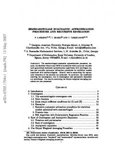
up to a multiplicative constant as n → ∞. These time-nets are introduced, for example, in [9, Chapter 6] and Theorem 7 implies that this choice is precisely deterθ mined by the spaces B2,2 (γ). As we will see the typical property of the time-nets τn

realizing the rate n−1/2 is that their knots concentrate more and more close to the time-horizon (see Figure 1. below). Theorem 7. [B, Theorem 3.2] Let θ ∈ (0, 1), f ∈ L2 (γ), and X be either the Brownian motion or the geometric Brownian motion. Then the following assertions are equivalent: θ (i) f ∈ B2,2 (γ).

(ii) There is a C2 > 0 such that, for all τ = (ti )ni=0 ∈ T , n X ∂ F (ti−1 , Xti−1 )(Xti − Xti−1 ) (f (W1 ) − Ef (W1 )) − ∂x i=1

≤ C2 sup

i=1,...,n

(ti − ti−1 )

(1 − ti−1 )

1 2

1−θ 2

.

(iii) There is a C3 > 0 such that, for all n = 1, 2, ..., n X ∂ (n,θ) F (ti−1 , Xt(n,θ) )(Xt(n,θ) − Xt(n,θ) ) (f (W1 ) − Ef (W1 )) − i−1 i i−1 ∂x i=1

L2

L2

C3 ≤√ n

14 where the nets τnθ are given by (n,θ) ti

1  i θ . := 1 − 1 − n

Optimal net 1 0.8 0.6 0.4 0.2

0.2

0.4

0.6

0.8

1

Equidistant net

Figure 1. Equidistant nets vs. Optimizing nets for θ = 3/4.

3. Multi-dimensional case In the final chapter we work in the multi-dimensional setting, d = 1, 2, 3, . . . We start with the diffusion (Yt )t∈[0,T ] , T > 0, given as unique solution of Yti

=

y0i

+

Z

0

t

ˆbi (Yu )du +

d Z X j=1

0

t

σ ˆij (Yu )dWuj , i = 1, . . . , d, a.s.

where ˆbi (x), σ ˆij (x) ∈ Cb∞ (Rd ) P ˆik (x)ˆ σjk (x), is uniformly elliptic i.e. and σ ˆσ ˆ T , where (ˆ σσ ˆ T )ij (x) = dk=1 σ d X

(ˆ σσ ˆ T )ij (x)ξi ξj ≥ λ ||ξ||2 , for all x, ξ ∈ Rd and some λ > 0.

i,j=1

15 The reason to start with this process is that under the above assumptions the process Y has a transition density Γ with appropriate tail estimates (cf. [2] and [3]) needed to prove our results. The process X is now defined in two cases by (Bm) Xt := Yt , (gBm) Xt := eYt , where we set ey := (ey1 , . . . , eyd ) for y ∈ Rd . The first case is related to the Brownian motion and the second one is close to the geometric Brownian motion. Now for some vector b and matrix σ the process X is of form Xti

=

xi0

+

Z

t

bi (Xu )du + 0

d Z X j=1

t 0

σij (Xu )dWuj , i = 1, . . . , d, a.s.

where x0 ∈ Rd . We notice that here we also allow a drift term in the underlying diffusion process for our approximation problem (which is sometimes remarked, but not carried out, in the literature). The multi-dimensional case was studied before by Zhang [20] and Temam [19] for equidistant nets. For certain C 1 -functions Zhang established the rate n−1/2 . On the other side, Temam proved the rate n−1/4 for the European digital option. The article [C] improves, for example, the approximation rate of the European digital option in the multi-dimensional case from n−1/4 to n−1/2 by replacing the equidistant nets by general deterministic nets. From Theorem 8 below it follows for a certain class of functions f that one gets the L2 -approximation rate of n−1/2 by optimizing over all deterministic nets of cardinality n + 1. To present our result we assume, for some q ∈ [2, ∞) and C > 0, that |f (x)| ≤ C (1 + ||x||q ) , x ∈ E, where f : E → R is a Borel-function and the set E is defined by   Rd , in case (Bm) E :=  (0, ∞)d, in case (gBm). The functions Qi : Rd → R for i = 1, . . . , d are defined by   1, in case (Bm) Qi (x) :=  xi , in case (gBm)

16 and the random variable f (XT ) has a representation f (XT ) = F (0, X0 ) +

d Z X k=1

T 0

∂ F (u, Xu )dXuk a.s. ∂xk

where F (t, x) := E(f (ZT )|Zt = x) with Z = (Zt )t∈[0,T ] being a solution of Zti

=

xi0

+

d Z X

0

j=1

t

σij (Zu )dWuj , i = 1, . . . , d, a.s.

Using this notation we have Theorem 8. [C, Theorem 1] Assume that for all x ∈ E ∂s Qi (x) q ∂x ∂ r σij (x) ≤ C1 Qq (x)Qr (x) , q + r = s, q, r, s ∈ {0, 1, 2} , β xα α β |bi (x)| ≤ C1 Qi (x) and (σσ T )ii (x) ≥

1 Q2 (x) C1 i

for i ∈ {1, . . . , d} and some fixed

C1 > 0. Moreover, assume that " sup E α,β

2 # 2 C2 ∂ F (t, Xt ) ≤ , θ ∈ [0, 1), (3.1) (σσ T )αα (Xt )(σσ T )ββ (Xt ) ∂xα xβ (T − t)2θ

for some C2 > 0. Then  2  12  d Z tη ∧t  n X X i D1 ∂ ∂ E sup F (u, Xu ) − F (tηi−1 , Xtηi−1 ) dXuk  ≤ √ , ∂xk ∂xk n t∈[0,T ] i=1 k=1 tηi−1 ∧t where

τnη :=

T

 1 !!n  i 1−η 1− 1− n

i=0

  η = 0, θ ∈ [0, 21 ) and  η ∈ (2θ − 1, 1), θ ∈ [ 1 , 1) 2

and D1 > 0 depends at most on η, C1 , C2 , d and T . In addition assume that

inf H 2 (u) = CH > 0,

u∈(r,s)

(3.2)

for some 0 ≤ r < s < T , where H is defined by H (u) := E 2

d X

(σσ T )αβ (Xu )(σσ T )ik (Xu )

α,β,i,k=1

Then we have following two cases:

∂2 ∂2 F (u, Xu) F (u, Xu ), u ∈ [0, T ). ∂xα xi ∂xβ xk (3.3)

17 (1) If θ ∈ [0, 3/4), then we have for any sequence of time-nets 0 = tn0 ≤ tn1 ≤ . . . ≤ tnn = T with supi=1,...,n (tni − tni−1 ) ≤ Cτ /n, Cτ > 0, that

n d Z n  2  12  t ∧t √ ∂ ∂ X X i k   F (u, Xu ) − F (ti−1 , Xti−1 ) dXu lim inf n E sup n→∞ ∂xk ∂xk t∈[0,T ] i=1 tn i−1 ∧t 

k=1

(3.4)

≥

1 . D2 (2) If θ ∈ [3/4, 1), then we have that

2  21  n X d Z tη,n ∧t  X i √ ∂ ∂ η,n k   η,n F (u, Xu) − F (ti−1 , Xti−1 ) dXu lim inf n E sup n→∞ ∂xk ∂xk t∈[0,T ] i=1 k=1 tη,n i−1 ∧t 

(3.5)

≥

1 . D2 The constant D2 > 0 depends at most on C1 , C2 , CH , d and T . We finish by some remarks concerning Theorem 8. The same results as in [9]

can be proved for the multi-dimensional case under the additional assumptions, for example, that σ ˆ is a diagonal matrix and that the process X does not have a drift. In the general multi-dimensional case the results from [9] cannot be straightforwardly extended because part of the arguments from the 1-dimensional case do not seem to apply in the multi-dimensional situation. The restriction θ ∈ [0, 3/4) in item (1) of Theorem 8 contradicts the intuitive understanding since larger θ should correspond to a worse approximation, however, we need the restriction for technical reason (but believe that it can be removed). Moreover, in reference [9] in the 1-dimensional case it has been shown that the error can be completely controlled by a certain deterministic function and that the optimal convergence rate is n−1/2 when optimized over deterministic nets of cardinality n + 1. The candidate for this function in the multi-dimensional case seems to be the function H defined in (3.3). Hence, for the future work, it would be worthy to clarify where this function H guarantees the same results as in [9], which would remove the restriction θ ∈ [0, 3/4) in item (1) of Theorem 8.

18 References [1] C. Bennett, R. Sharpley: Interpolation of Operators. Academic Press, 1988. [2] A. Friedman. Partial Differential Equations of Parabolic Type. Prentice-Hall, 1964. [3] A. Friedman. Stochastic Differential Equations and Applications. Academic Press, Vol. 1, 1975. [4] H. F¨ollmer, P. Leukert: Efficient hedging: Cost versus shortfall risk. Finance and Stochastics 4:117-146, 2000. [5] H. F¨ollmer, P. Leukert: Quantile hedging. Finance and Stochastics 3:251-273, 1999. [6] C. Geiss, S. Geiss. On approximation of a class stochastic integrals and interpolation. Stochastics and Stochastic Reports, 76 (4):339-362, 2004. [7] C. Geiss, S. Geiss. On an approximation problem for stochastic integrals where random time nets do not help. Stochastic Processes and their Applications, 2005. [8] S. Geiss. On quantitative approximation of stochastic integrals with respect to the geometric Brownian motion. Report Series: SFB Adaptive Information Systems and Modelling in Economics and Management Science, Vienna University, 43, 1999. [9] S. Geiss: Quantative approximation of certain stochastic integrals. Stochastics and Stochastics Reports, 73:241-270, 2002. [10] S. Geiss: Weighted BMO and discrete time hedging within the Black-Scholes model. Probability Theory and Related Fields 132:13-38, 2005. [11] E. Gobet, E. Temam: Discrete time hedging errors for options with irregular payoffs. Finance and Stochastics, 5:357-367, 2001. [12] T. Hayashi, P. Mykland: Evaluating hedging errors: an asymptotic approach. Mathematical finance, 15 (2):309-343, 2005. [13] D. Bertsimas, L Kogan, A. Lo: When is time continuous? Journal of Financial Economics, 55:173-204, 2000. [14] D. Bertsimas, L Kogan, A. Lo: Hedging derivative securities and incomplete markets: an ε-arbitrage approach. Operations Research, 49 (3):372-397, 2001. [15] I. Karatzas, S. Shreve: Brownian motion and stochastic calculus. Springer-Verlag 1988. [16] D. Lamberton, B. Lapeyre: Introduction to stochastic calculus applied to finance. Chapman & Hall, 1996. [17] H. Rootzen: Limit distributions for the error in approximations of stochastic integrals. Ann. Prob. 8:241-251, 1980. [18] M. Schweizer: A guided tour through quadratic hedging approaches. Handbooks in Mathematical Finance: Option Pricing, Interest Rates and Risk Management. Cambridge University Press, 2001. [19] E. Temam. Analysis of error with malliavin calculus: Application to hedging. Mathematical Finance, 13 (1):201-214, 2003.

19 [20] R. Zhang: Couverture approche des options Europennes. PhD Thesis, Ecole Nationale des Ponts et Chauss´ees, Paris, 1998.