Dec 14, 1995 - In the literature on counting string solutions to Bethe equations, distinct integers ...... [32] P. Goddard, A. Kent and D. Olive, Comm. Math. Phys.
arXiv:hep-th/9512095v2 14 Dec 1995
On the combinatorics of row and corner transfer (1) matrices of the An−1 restricted face models Srinandan Dasmahapatra Department of Mathematics, City University, London, EC1V 0HB, UK December 1995 Abstract We establish a weight-preserving bijection between the index sets of d the spectral data of row-to-row and corner transfer matrices for Uq sl(n) restricted interaction round a face (IRF) models. The evaluation of momenta by adding Takahashi integers in the spin chain language is shown to directly correspond to the computation of the energy of a path on the weight lattice in the two-dimensional model. As a consequence we derive fermionic forms of polynomial analogues of branching functions for the (1)
cosets
(1)
(An−1 )ℓ−1 ⊗(An−1 )1 (1) (An−1 )ℓ
, and establish a bosonic-fermionic polynomial
identity.
1
Introduction and Summary
The basic object of interest in the statistical mechanics of a large number of classically interacting degrees of freedom in d Euclidean space-time dimensions is the partition function, which is the generating function of all correlation functions. The calculation of the partition function requires the (Boltzmann) weighted sum over all configurations of the system, and can be generated by a transfer matrix. From the transfer matrix, it is possible to extract the definition of an interacting hamiltonian for a quantum system in (d − 1) spatial dimensions. Even though the physical interpretation in the two cases is often very different, techniques developed for investigation in one framework can be adapted to extract useful information in another. For d = 2, there have been very striking recent advances in the study of exactly solvable models which do precisely this.
1
The method of introducing the corner transfer matrix (CTM) [1] for the calculation of order parameters [2, 3, 4, 5] has spawned the development of quantum affine Lie algebraic tools for the study of correlation functions, after the realization that the CTM density is closely related to the derivation in the affine algebra [6, 7]. These have then been applied to the study of XXZ (for c2 )) and higher rank infinitely long quantum chains. Among other results, Uq (sl this method has provided a mathematical (representation theoretic) grounding to the notion of a “quasi-particle” [8] in this model [7]. The concept of a quasi-particle is a key physical ingredient in the intuition built into the search for collective modes which appear as summands in the additive decomposition of the energy and momentum of the many-body system in the thermodynamic limit. In the context of the ferromagnetic XXX Heisenberg chain, a magnon or spin-wave describes a linear combination of states that have this additive character, and is called an elementary excitation. For the anti-ferromagnetic chain, the Bethe ansatz approach requires filling the “Fermi sea”1 with “pseudo-particles” (magnonic or spin-wave states) and looking for “dressed” particle and “hole” excitations (filling an unfilled state, or evacuating an occupied one), above the Fermi sea. The concept of “spinons” that emerged from this picture [8] was put into the language of representation theory in [7], in terms of the span of a momentum-indexed set of eigenstates related by nonAbelian symmetries of the hamiltonian. There has been another set of developments in the past few years which have conjectured [9, 10] (and proven in some cases [11, 12]) that certain generating functions of momenta of fermionic quasi-particle excitations above a ground state in quantum chains coincide with the low-temperature expansions of the order parameter in the associated 2-dimensional models. In the case of quantum spin chains, the eigenvalues of the row transfer matrix (RTM) were studied. It was the observation that these order parameters of the 2-dimensional models were, in fact, branching functions of cosets of affine Lie algebras that led to the development and implementation of ideas from representation theory. It seems equally likely that the calculation of the spectrum of the RTM approach may be similarly recast in more mathematically precise terms. Both the CTM and RTM calculations under consideration are essentially combinatoric in nature, i.e. both involving counting objects in a certain class. Namely, in the CTM approach, what is evaluated is a weighted sum of a set of paths on the weight lattice of the appropriate quantum affine algebra which index the eigenvectors of the CTM, whereas in the RTM calculations, the weighted sum performed is over the configurations of strings and holes which characterize solutions to the Bethe equations, on which the eigenvalues of the RTM depend. In this paper, we pursue the idea that since both these combinatorial approaches give the same answer, there must be a bijection between the sets being counted. In a number of cases [12] bijective proofs have been provided for polynomial 1 This
terminology is borrowed from the description of many-fermion systems.
2
analogues of these branching function identities. However, they do not address the issue of mapping the objects counted in the two different cases into each other. It was observed in [13, 14] however, that one could write down an explicit bijection between these two sets of objects, based on an algorithmic construction given in a remarkable paper [15]. The face models that were studied were (1)
related to the cosets
(1)
(An−1 )ℓ−1 ⊗(An−1 )1 (1) (An−1 )ℓ
, for the cases arbitrary n, ℓ = 2 and
arbitrary ℓ, n = 2. The present paper extends this idea to arbitrary (n, ℓ). The two solutions, for the CTM and RTM approaches, that exist in the literature for these models are those of the order parameters in [5] and the spectrum and thermodynamics in [16].
1.1
Finite size approximations
The bijection [15] of this paper and [14] is established for finite chains, where we do not have the full affine symmetry. This may be viewed as an approximation of the infinite lattice case in a certain sense to be explained below. Reference [15] established a bijection between the “rigged configurations” which parametrize Bethe vectors, which are highest weight vectors of gl(n) (for gl(n) invariant models) and the well-known index set of highest weight states of gl(n), namely, Young tableaux [17]. These “rigged configurations” were based on the ‘string hypothesis’ [19] form of the solutions of the Bethe equations, the counting method of [20] generalized for the higher rank models [21]. By Schur-Weyl duality, the cardinality of these sets is the dimension of the irreducible representation of SL , the symmetric group on L letters (L is the size of the system), labelled by the partition λ of L. This is called the Kostka number, Kλµ the number of tableaux of shape λ and weight µ, where µ = 1L and λ ⊢ L. It can be expressed in terms of a vector partition function π(µ), defined by Y
α∈R+
X 1 = π(µ)eµ , α 1−e µ
which counts the number of ways of writing a weight µ as a sum of positive roots α ∈ R+ . The Kostant multiplicity formula2 X � nµ (Γλ ) = (−1)l(w) π w(λ + ρ¯) − (µ + ρ¯) , (1) ¯ w∈W
gives the number of times the weight µ occurs in the irreducible representation Γλ labelled by the highest weight λ. Here ρ¯ is half the sum of the positive ¯ is the Weyl group for the root system of the Lie algebra, and and any roots, W ¯ w ∈ W can be expressed as a product of l(w) elementary reflections, where l(w) ¯ . For the An−1 root system, nµ (Γλ ) = Kλµ is called the length of the word in W ¯ and W is isomorphic to the symmetric group. 2 This
is in fact equivalent to the Weyl character formula.
3
The bijection of reference [15] established the “completeness” of Bethe ansatz states by demonstrating that the number of Bethe states was indeed equal to the Kostka number. In other words, this established that the “bare” or “pseudoparticle” description of the spectrum, as an assembly of spin-wave-like states accounted for all the states in any finite system, 3 so that the “dressed” quasiparticle states above the ground state would guarantee the completeness of the particle picture in the emergent theory in the thermodynamic limit. The spectral decomposition of all correlation functions in this theory would involve summing over these quasi-particle states. The vector partition function may be refined as follows: Y X 1 = πq (µ)e(µ), 1 − qe(α) + µ α∈R
where the coefficient of q k in πq (µ) counts the number of ways a weight µ can be expressed as a sum of k positive roots α ∈ R+ . The q-analogue of the Kostant multiplicity formula, X � (2) ε(w)πq w(λ + ρ¯) − (µ + ρ¯) , Kλµ (q) = ¯ w∈W
is the Kostka-Foulkes polynomial.4 Kλµ (q) are the entries of the transition matrix between two bases in the ring of symmetric functions in a denumerably infinite set of independent variables X = x1 , x2 , . . ., namely the Schur function sλ (X), and Pλ (X; q) called the Hall-Littlewood function X sλ (X) = Kλµ (q)Pλ (X; q). (3) µ
Explicitly, for xn+i = 0 for i = 1, 2, . . . in X and λ = (λ1 , . . . , λn ) a partition of length ≤ n. Y xi − qxj � X � 1 w xλ1 1 · · · xλnn Pλ (X; q) = vλ (q) xi − xj i 1. Note the cyclic property of the Dynkin diagram Λi+kn = Λi for all integer k. Thus, the multiplicities of weights in the module of the affine algebra may be approximated by a consideration of corresponding Kostant formulas for the finite dimensional modules of Uq sln . In fact, such an analog of Kostant’s qmultiplicity formula has been considered in [5] where the weight (the exponent of q) is given by the ‘energy function’ obtained by taking the q = 0 limit of the Boltzmann weights of these restricted models. This is used to evaluate the eigenvalue of the CTM at q = 0, when the paths diagonalize the CTM hamiltonian. It was established in [5] that for a finitized path, or sequence of Pn−1 weights µ = (µ0 , µ1 , . . . , µL , µL+1 ), such that eachP µj is of the form i=0 mi Λi and the mi s are non-negative integers satisfying i mi = ℓ, and µi+1 − µi = Λj −Λj+1 for some j, the following is true. For a section of a path (µi , µi+1 µi+2 ) where µj ∈ P , one can define a local energy function H, from the q = 0 (low temperature) limit of the Boltzmann weights: H(Λ, Λ + ˆ, Λ + ˆ + ˆı) = θ(ı − ), where ˆ := (Λj+1 − Λj ) for = 0, 1, . . . , n − 1 and θ is the step function given by � 0 (z > 0) θ(z) = 1 (z ≤ 0). In order to compute the one-point functions of the restricted face models of the following weighted sum over the set of paths µ was calculated in [5]: PL−1 X q k=0 (k+1)H(µk ,µk+1 ,µk+2 ) , (6) XL (a, b, c; q) =
(1) An−1 ,
{µ|µ0 =a,µL =b,µL+1 =c}
6 This
is developed further in refs. [31] where the theory of perfect and affine crystals is introduced.
6
where the steps µk of the path belong to the set P + (n; ℓ) = {Λ =
n−1 X
mi Λi |mi ∈ Z, mi ≥ 0,
n−1 X
mi = ℓ}
i=0
i=0
of dominant integral weights. For b = ξ + σ L (η), for ξ ∈ P + (n; ℓ − 1), η ∈ P + (n; 1),
c = b + Λk+1 − Λk ,
it was found that XL (a, b, c; q) =
X
1
(−1)l(w) q 2 |ξ+ρ−w(a+ρ)|
2
+cL
w∈W
where {αi } satisfies the relations n−1 X
αi = L, and
i=0
ρ= and
Pn−1 i=0
n−1 X
[L]! , Qn−1 i=0 [αi ]!
(7)
αi (Λi+1 − Λi ) ≡ b + ρ − w(a + ρ) mod δ,
i=0
Λi = ρ¯+ nΛ0 , W is the affine Weyl group, l(w) is the length function,
1 (L − j)(L + n − j). 2n The inner product on the weight lattice used above is given by cL (j) =
hΛi , Λj i = min(i, j) −
(8)
ij =: G−1 ij , hδ, δi = 0 and hδ, Λi i = 1. n
By the isomorphism between the crystal graph of the highest weight repcn and the appropriate construction of the action of the resentations of Uq sl Kashiwara endomorphisms on the CTM paths [29], the L → ∞ limit of these (1)
polynomials gives the branching functions of the cosets χξ (z1 , . . . , zn ; q)χη (z1 , . . . , zn ; q) =
X
(1)
(An−1 )ℓ−1 ⊗(An−1 )1 (1) (An−1 )ℓ
:
bξη a (q)χa (z1 , . . . , zn ; q),
a
in the principal specialization (zi = q 1/n ) where χα are the characters of the irreducible modules with highest weight α. (For expressions for χa and babc , see [5].) Explicitly, we have lim q φL XL (a, b, c; q) = bξη a (q)
L→∞
� where φL = L (L/n) − 1 /2 + γ(ξ, η, a), γ(ξ, η, a) :=
|ξ + ρ|2 |η + ρ|2 |a + ρ|2 |ρ|2 + − − . 2(ℓ + n − 1) 2(n + 1) 2(ℓ + n) 2n 7
(9)
The presence of alternating signs in (7) which carries over to the branching functions in the limit, is explained as the elimination of states from the (n − 1) free bosonic Fock space realization of the Verma modules [34, 33], and is hence called a bosonic form of the branching function. In this paper, we prove the equality of the polynomials XL (ℓΛ0 , ℓΛ0 , (ℓ − 1)Λ0 + Λ1 )(q) and the sum (28) below, whose terms have manifestly positive coefficients, called a fermionic form. This polynomial was first written down in [35] and its equality with (7) conjectured in [36], in the spirit of [37]. The proof is based on two observations. It is well known [18] that for standard tableaux, the statistics charge (mentioned earlier) and p introduced in [40] are equidistributed. It was observed in [14] that p evaluated on a standard tableau designed to encode a path is identical to the energy function P L−1 j=0 (j + 1)H(µj , µj+1 , µj+2 ) evaluated on the same path. The second observation is the property of the bijection of [15] that it respects the level of the integral weights in a certain sense. Namely, for a tableau encoding a restricted path of level ℓ, it can be proved that the maximum length of string allowed in the bijectively associated configuration of strings and holes is ℓ, as was conjectured in [16] after numerical investigation of the solutions of Bethe’s equations. This immediately leads to the proof of the polynomial identity, Theorem 1 (bosonic-fermionic polynomial identity) 1
L
q − 2 L( n −1) XL−1 =
ℓ X n−1 YY
1
q 2 (h|h)
{ν} a=1 j=1
where (h|h) =
X
�
(a)
hj
+
P P b
(b) −1 k Gab Cjk hk (a) hj
�
,
(10)
(a) (b)
G−1 ab Cjk hj hk ,
ab ; jk
and Cjk = (2δjk − δj(k−1) − δj(k+1) ). The paper is organized as follows. We give the basic definitions of the model and describe the CTM paths in section 2, and how to encode them as standard tableaux. In section 3, we define functionals on the set of paths and tableaux, and demonstrate the relationship between them. In section 4, we introduce the ‘rigged configurations’ and in sections 5 and 6, we describe the bijection of [15], and another version [38] of the same, which is cast in the familiar language of strings and holes, and has a pictorial character. In section 7, we evaluate the momenta of the Bethe states in terms of a sum of Takahashi integers, and prove that this gives the charge or p of the corresponding tableau. Here we give the proofs omitted in [22, 24]. This leads immediately to the proof of the equidistribution of energies of CTM paths and momenta of Bethe states. This is stated in section 8, after which we end with a small discussion.
8
2
The state space, tableaux and paths.
In RSOS models, the ‘spin’ degrees of freedom assigned at each node of the lattice take on any values from the set (state space) P + (n; ℓ), whose elements d Explicitly, we state are the level ℓ dominant integral weights (DIW) of sl(n). Definition 1 (State space) For Λi , i = 0, . . . , n − 1 the fundamental weights d and some natural number ℓ, of sl(n), P (n; ℓ) = {Λ =
n−1 X
mi Λi |mi ∈ Z,
n−1 X
mi = ℓ}
i=0
i=0
is the set of integral weights, and the state space is P + (n; ℓ) = {Λ =
n−1 X
mi Λi ∈ P (n; ℓ)|mi ≥ 0}.
i=0
Let ǫj = (0, · · · , 0, 1, 0, · · · , 0) be an n-dimensional vector with 1 in the j th position, j = 0, . . . , n − 1, and define the set A+ ℓ : A+ ℓ = {ν =
n−1 X
νi ǫi |νi ∈ Z, νi ≥ 0,
n−1 X
νi = ℓ}.
i=0
i=0
The subscript i of Λi , ǫi may be extended to i ∈ Z by setting Λi = Λj and ǫi = ǫj for i ≡ j (mod n). The configurations of states that label the eigenvectors of the corner transfer matrix (CTM) are those that dominate the partition function in the low temperature limit. These low-temperature configurations are best described by a set of paths which we define below. Definition 2 (Path, Λ-path) A path is a pair (µ, η) such that 1. µ = (µk )k≥0 , µk ∈ P (n; ℓ) 2. η = (ηk )k≥0 , ηk ∈ A+ ℓ and 3. µk+1 − µk = η¯k ∀k, where − : A+ ℓ → P0 is a Z-linear map which maps ǫj 7→ ǫ¯j = Λj+1 − Λj . A Λ-path is a path as above, such that µk = σ k (Λ) for k >> 0 and where σ(Λj ) = Λj+1 ∀j. In fact, the class of paths we shall focus on in this paper are a subset of those described above.
9
Definition 3 (Restricted paths [29]) Let Λ, Λ′ be dominant integral weights of level l, l′ respectively. A (Λ′ , Λ) path is defined as a pair of sequences (µ, η) such that 1. (µ − Λ′ , η) is a Λ-path, and 2. µk −ˇηk ∈ P + (n; ℓ′ ) ∀k ≥ 0, where ˇ: A → P is a Z-linear map which maps ǫj 7→ ˇǫj =Λj . Unpacking the definitions a little, we note that whereas a path is defined as a cn , the restricted paths are sequences of domisequence of integral weights of sl nant integral weights (often abbreviated as DIW). This is the key feature that distinguishes vertex from RSOS models. We can give an equivalent definition as follows of restricted paths emphasizing this difference. Definition 4 (Restricted paths, again) For DIWs Λ ∈ Pl+ , Λ′ ∈ Pl+ ′ , (µ, η) is a (Λ′ , Λ)-path iff + 1. µ = (µk )k≥0 µk ∈ Pl+l ′,
2. µk = Λ′ + σ k (Λ) for k >> 0, 3. η = (ηk )k≥0 ηk ∈ A+ l and 4. µk+1 − µk = η¯k , where A¯l and σ(Λ) are defined above. In this paper, we shall only consider the cases l′ = ℓ−1, l = 1. Therefore, only the specification of the sequence ηk ∈ {ǫj }0≤j≤(n−1) is sufficient to characterize a Λ-path. Let us denote the set of all such restricted paths as Pℓ (Λ′ , Λ). A ground state path for this class of (fundamental) models we shall consider in regime III of the parameter space, is a (Λ′ , Λ) path with η GS = (ηi+kn = ǫi ) for k ≥ 0 and 0 ≤ i ≤ (n − 1). In other words, µk = (Λ′ − Λ0 ) + σ k (Λ0 ) is a ground state path for any choice of Λ′ ∈ P + (n; ℓ). The set of all paths in Pℓ (Λ′ , Λ) for which (µk , ηk )k≥L+1 is a ground state path, is called a finitized path, and is denoted PℓL (Λ′ , Λ). It is customary to strip off the semi-infinite tail of the sequence which is indistinguishable from the ground state sequence. In this paper, we shall describe a state by a Young diagram, λ = (λ1 , . . . , λn ), where λ1 ≥ · · · ≥ λn and λ1 −λn ≤ ℓ. Let the set of all such diagrams be denoted Yn,ℓ . A dominant integral weight is represented by such a diagram, and the map wt:Yn,ℓ → P + (n; ℓ), defined as wt(λ) =
n−1 X
(λi − λi+1 )Λi ,
i=0
where λ0 := ℓ − (λ1 − λn ). 10
∅
Figure 1: The oriented graph G with the Young diagrams at the nodes representing DIWs. We shall translate the definition of restricted paths into the language of Young diagrams as follows. Let us introduce an oriented graph G, the set of whose nodes is P + (n; ℓ) and whose oriented bonds (or arrows) are drawn as follows. For a, b ∈ P + (n; ℓ), we draw an arrow between a and b if b − a = ǫ¯i = Λi+1 − Λi ∈ A¯+ 1 , for some i = 0, . . . , n − 1. ǫ¯j , for j = 1, . . . , n − 1 may be identified with the weights of the fundamental representation of sln (C). In terms of Young diagrams, α, β ∈ Yn,ℓ , with wt(α)= a and wt(β)= b are connected by an arrow from α to β if β is obtained by adding a box to the i + 1th row of α. Thus, for some k, µk = a = wt(α), µk+1 = b = wt(β) and ǫ¯i is described by the extra box in the i + 1th row.
2.1
Paths as tableaux
A standard Young tableau T is a Young diagram whose cells are occupied by integers that increase along rows and columns. Definition 5 (Lattice permutation) A word or multiset permutation w of the letters 0, . . . , (n − 1), is called a lattice permutation if, on reading from left to right, the number of occurences of i in w is no less than that of j, for all i < j. For a given sequence of integers labelling a path, η(p) is a multiset permutation. We shall encode such a path η(p) = (η1 , . . . , ηL ) as an array by the following procedure. We place the integer j in the (i + 1)th row of an array 11
iff ηj = ˆi. For restricted paths which are sequences of DIWs, the array thus formed is of partition shape, and are Young tableaux, and are thus lattice permutations. We can stick to normal standard tableaux in this paper (not skew shapes) unless we specify otherwise, with the first integer in η(p) = ˆ0. To a path p, we denote by Tp the tableau associated to it by this procedure,and to any tableau T , We call wT the lattice permutation corresponding to T , so that p = wTp . Example. The following sequence of Young diagrams ǫ¯
0 ∅ →
ǫ¯
0 →
ǫ¯
1 →
ǫ¯
ǫ¯
ǫ¯
1 →
0 →
2 →
ǫ¯
0 →
ǫ¯
1 →
ǫ¯
1 →
encodes the restricted path or sequence of DIWs ℓΛ0
ǫ¯
0 → (ℓ − 1)Λ0 + Λ1 ǫ¯2 → (ℓ − 1)Λ0 + Λ1 ǫ¯0 → (ℓ − 3)Λ0 + 2Λ1 + Λ2
ǫ¯
0 → (ℓ − 2)Λ0 + 2Λ1 ǫ¯0 → (ℓ − 2)Λ0 + 2Λ1 ǫ¯1 → ···
ǫ¯
1 → (ℓ − 2)Λ0 + Λ1 + Λ2 ǫ¯1 → (ℓ − 2)Λ0 + Λ1 + Λ2
as does the following Young tableau 1 3 4
2 5 6 8
7 .
We also note that any tableau T representing some path p ∈ PℓL contains L boxes, and any partial tableau T (k) of T is the sub-diagram that contains the first k integer entries. For example, for T as above, L = 8 and the partial tableau T (5) is 1 2 5 T (5) = 3 . 4 Also, for most of the paper we shall be focusing on the vacuum module for (1)
the cosets
(1)
(An−1 )ℓ−1 ⊗(An−1 )1 (1) (An−1 )ℓ
and therefore [29], we focus on PℓL (ℓΛ0 , Λ0 ). In
terms of Young diagrams this means that a path begins at the empty diagram ∅ and after L = kn steps (for some positive integer k), comes back to ∅. Therefore, η contains an equal number of ǫj s for j = 0, 1, . . . , n − 1, and the shapes of the corresponding tableaux are thus rectangular, (k n ). The physical model is defined by the Boltzmann weights, and these are non-zero for a given specification of states on the adjacent sites of the physical (two-dimensional) lattice. This condition on nearest neighbour states can be expressed in terms of the oriented graph structure on P + (n; ℓ). Namely, for some given natural number f , a(n ordered) pair of states can occupy nearest neighbour sites on the lattice, if it takes at most f steps to go from a to b in P. f is called the degree of fusion, and as mentioned before, we shall only consider the case f = 1 in this paper. 12
3
Functionals on paths and tableau
We define an energy function H on a path as follows. Definition 6 (energy of a path) The energy of a path p, E(p) is given by the the evaluation of a functional H(p), H(p) =
L X
jθ(ηj − ηj−1 ),
(11)
j=1
relative to its evaluation on the ground state path p¯: E(p) = H(p) − H(¯ p) and θ is the step function given by � 0 θ(z) = 1
(12)
(z > 0) (z ≤ 0).
(13)
It is also useful to state the following convention for later usage: for a section of a path (µi , µi+1 µi+2 ) given by the three integral weights (λ1 , Λ2 = Λ1 + ǫ¯j , Λ3 = Λ1 + Λ2 + ǫ¯k ), one can define a local energy function: H(Λ1 , Λ1 + ǫ¯j , Λ1 + ǫ¯j + ǫ¯k ) := θ(k − j). Note that for a given p, the contribution to E(p) of each step j of the path is zero if the integer (j + 1) lies below j in Tp . With this property in mind, we introduce two integer-valued functionals or statistics on tableaux, c(T ) and p(T ). Definition 7 (Charge of a tableau [23]) For a row of a tableau T , assign an index i to each ai as follows. if 0 index(x) + 1 if index(aj = x + 1) := index(x) otherwise
word πT = a1 a2 . . . aL x=0 ai = x and i < j .
The charge c(πT ) of a word w = πT is
charge(πT ) :=
L X
index(ai ),
i=1
and the charge of a tableau c(T ) = c(πT ). In words, if the number x has index i, then x + 1 will have index i + 1 if it is to the right of x, and i otherwise. In order to define the statistic p(T ) it is necessary to set up the following definitions. For any permutation w of {1, 2, . . . , L} introduce the following sets:
13
Definition 8 (D(w), Dt (T )) (i) If j and j + 1 are both in w, D(w) = {j|j + 1 lies to the left of j in w}. P We also set d(w) = |D(w)| and des(w) = j∈D(w) j. (ii) For a tableau T , Dt (T ) = {j|j + 1 lies below j in T }. Definition 9 (Row word of a tableau [39]) For a tableau T , the row word πT of T is the permutation πT = Rn Rn−1 . . . R1 where Ri , i = 1, . . . , n are the rows of T read from left to right. Example. 1 T = 2 8
3 5 4 7
6 πT = 82471356
Note that Dt (T ) = D(πT ), and we shall drop the superscript on Dt and use the same notation D to refer to the map on both domains, words and tableaux. Also, set d(T ) = d(πT ) and des(T ) = des(πT ). Example. For T as above, D(T ) = D(πT ) = {1, 3, 6, 7}, d(πT ) = 4 and des(πT ) = 17. Remark. The row word of a tableau is a convenient index [39] for a Knuth (or plactic) equivalence class. This is a set of words that are related to each other by the Knuth relations [42] (or plactic monoid). Every word in each Knuth class gives the same P tableau under the Robinson-Schensted-Knuth correspondence. Definition 10 (statistic p(T) [40]) For a tableau T , introduce the set ET = {j|j + 1lies to the right of j in T }, P and define p(T ) := j∈ET j.
Remark. Observe that for a standard tableau T , D(T ) ∩ ET = ∅. In words, for every entry j in a standard tableau, (j + 1) lies either to the right of or below j, but not both. Example. For T as above, the indices for 1, 2, . . . , 8 are 0, 0, 1, 1, 2, 3, 3, 3 respectively, and c(T ) = 13. Remark. The statistics c(T ) and p(T ) are invariant under the Knuth relations.
14
3.1
Energy of a path as statistic p
Observe that for a path η GS := (0, 1, . . . , n − 1, 0, 1, . . . , n − 1, . . . , 0, 1, . . . , n − 1), of length L = nx (say), if the corresponding tableau is Tgs , then ETgs = {n, 2n, . . . , (x − 1)n}. Note, that if we treat every path p as a finite one, then L 6∈ ETp . Proposition 1 For a path η = (η1 , . . . , ηL ) encoded as a Young tableau T with |shT | = L = nx for x a natural number. The energy of the path E(η) is then E(η) = p(T ) −
L L ( − 1). 2 n
Proof: Observe p(Tp ) = H(p). For ease of computation, it is convenient to note
2
Proposition 2 (i) c(T)= 21 L(L − 1) − Ld(T ) + des(T ); (ii) p(T)= 12 L(L − 1) − des(T ). Proof: (i) Observe � that the contributions to c come from the sum 0 + 1 + · · · + L − d(πT ) − 1 and also from the set D(πT ). Namely, if x is the ith element of D(πT ), then index(x)= (x − i). Thus � c = 0 + 1 + · · · + (L − d − 1) + des(πT ) − (1 + 2 + · · · + d) ,
and the result follows. (ii) See the remark following the definition of p(T).
2 For future reference we shall introduce the following notation. Definition 11 For a standard tableau T , with |sh T | = L, � 1 I(T, L) := des(T ) − Ld(T ) . 2 Therefore, we can write c(T ) = p(T ) =
3.2
1 2L 1 2L
� L − 1 − d(T )� + I(T, L) . L − 1 − d(T ) − I(T, L)
(14)
An involution on tableaux: evacuation
The involution we shall describe is a special case of a family of operations which are indexed by points p ∈ Z × Z occupied by an ordered set of objects on which they act injectively. These were defined by Sch¨ utzenberger and are called jeu de taquin. For the involution S on standard tableaux, (also called evacuation), 15
the point in question is the top left corner (1, 1), e.g., the cell occupied by the number 1 in our example above. The operation S is defined by the following set of moves. First, remove the entry in cell (1, 1). Move the smaller of the two integers immediately below or to the right of it to occupy the cell (1, 1). This leaves a vacancy in the cell from which the integer was moved. Then look for the smallest integer immediately below or to the right of this freshly vacated cell, and move that one in to squat in it. This leaves a new cell empty. In general, whenever the cell (i, j) is empty, and t(i1 , j1 ) = min(t(i + 1, j), t(i, j + 1)), slide the integer from (i1 , j1 ) to (i, j). And so on, until there are no more cells to the right and below the cell vacated. In this last cell insert the number n with parentheses around it, to distinguish it from the n that is already present in the tableau. Now, remove the (new) integer from the cell (1, 1), and repeat this game, inserting (n − 1) in the last cell. And so on, until all the entries of the original tableau are deleted, and we have parentheses around the integers in the new standard tableau, which we then remove. Example. [evacuation] In the tableau T above, remove the entry from the cell (1, 1) and start the game: · 3 5
2 4 6 9 7
8
2 → 3 5
· 6 7
4 8 2 4 9 → 3 6 5 7
· 8 2 9 → 3 5
4 8 6 9 7
• .
Replace the • by (9). Iterating this one more time, we get · 3 5
4 8 6 9 7
(9)
3 4 → · 6 5 7
8 (9) 3 4 9 → 5 6 · 7
8 (9) 3 4 9 → 5 6 7 •
8 (9) 9 .
After a couple of more steps, we have 3 5 7
4 8 (9) 4 6 8 (9) 5 6 8 (9) 6 9 9 (7) → 5 9 (7) → 7 , (8) 7 (8) (6) (8)
and so on until
1 3 TS = 2 4 6 8
5 9 7 .
Check that S is an involution, i.e. S 2 = 1, or (T S )S = T . Proposition 3 For tableaux T and T S related by the evacuation involution, c(T ) = p(T S ). Proof: See [41]. Give proof here. Remark. As a trivial corollary to the above, note that I(T, L) = −I(T S , L). 16
2 (15)
4
Introducing Rigged Configurations.
Let λ and µ be partitions such that |λ| = |µ| and the number of parts ℓ(λ) d ℓ−f ⊗ of λ is no bigger than n. Since we are interested in the cosets (sl(n)) d f /(sl(n)) d ℓ for the fusion level f = 1 in this paper, we choose µ = (1L ) to (sl(n)) indicate that the state space is chosen from the summands in the decomposition of an L-fold tensor product of fundamental representations of sln (C). For a given λ one can define a sequence of partitions ~ν = (ν (0) , ν (1) , . . . , ν (n−1) ) which satisfy the condition |ν (a) | =
X
λk .
(16)
k≥a+1
We set ν (0) = µ = 1L . We shall call the rows of a partition ν (a) strings of colour a. Let l∗ be the maximum allowed length of string, sj (ν (a) ) be the number of (a) strings of colour a and length j, and Qj (ν) be the number of cells in the first P∗ (a) (a) min(i, j)si . j columns of diagram ν (a) , i.e. Qj = li=1 (a)
To every string in ν (a) is assigned an integer Jj,α , α = 1, . . . , sj (ν (a) ), a = (a)
1, . . . , n − 1 and j = 1, . . . , l∗ , called a rigging. These integers Jj,α are chosen (a)
(a)
from the set {0, 1, . . . , hj }. The maximum allowed integer, hj number of holes of colour a and length j, and is determined by: (a)
hj (a)
We must have hj
(a−1)
= Qj
(a)
(a+1)
− 2Qj + Qj
is called the
,
(17)
≥ 0 for a configuration to be admissible.
Definition 12 (rigged configurations) A configuration of partitions ν whose (a) (a) rows are indexed by non-negative (i.e., admissible) integers Jj,µ , µ = 1, . . . , sj (a)
(a)
no larger than hj for 1, ≤ j ≤ l∗ where hj is calculated as above is called a rigged configuration. We shall denote a rigged configuration by (~ν , {J}) where {J} denotes the set of rigging integers. The total number of admissible rigged configurations is given by l∗ � (a) (a) � X n−1 YY sj + h j . (a) sj {ν} a=1 j=1
(18)
Recall that the number of holes is calculated once the number of strings is known, using X (a+1) (b) (a) (a−1) (a) = Lδa1 − Gab Qj , − 2Qj + Qj hj = Q j b
17
where Gab are the matrix elements of the Cartan matrix of sln . Inverting the above equation, we get X (a) (b) Qj = LG−1 G−1 a1 − ab hj , b
P (a) (a) (a) which, together with the relation Qj − Qj−1 = k≥j sk , may be used to express the number of strings in terms of the number of holes. Note, X X (b) ¯ (a) := h(a) − h(a) = Gab sk , (19) h j+1 j j b
so that
(a)
sj
= =
(a)
(a)
k≥j+1
(a)
(a)
(Qj − Qj−1 ) − (Qj+1 − Qj ) P P −1 (b) LG−1 a1 δj1 − b k Gab Cjk hk ,
(20)
where Cjk = (2δjk − δj (k−1) − δj (k+1) ). Remark. In the literature on counting string solutions to Bethe equations, distinct integers are assigned to strings [20], unlike the rigging defined here. The relation between the distinct (also called fermionic) (half-)integer branches (a) (a) Ij,α and the not necessarily distinct rigging integers Jj,α is given by 1 (a) (a) (a) (a) Ij,α = Jj,α + α − (hj + sj + 1). 2
5
(21)
The Kerov-Kirillov-Reshetikhin Algorithm
In a remarkable paper [15], a bijection between standard Young tableaux and rigged configurations was established. In [22] and [24] this was extended to a charge preserving bijection between tableau of shape λ and weight µ a partition. We shall concentrate only on standard tableaux for the purpose of this paper. We shall describe this bijection in this section. Let SYT(λ) be the set of standard Young tableau of shape λ and Rλ be the set of admissible rigged configurations {~ν , {J}} satisfying the condition (16). We shall describe the monomorphisms (injective maps) τ : Rλ −→ SY T (λ) and ρ : SY T (λ) −→ Rλ , with τ ◦ ρ = ρ ◦ τ =id. We shall usually drop the subscript on R.
5.1
ρ : SY T (λ) −→ R.
We shall describe the map from wT , T ∈ SY T (λ) to an admissible rigged configuration. The construction is inductive – let there be a rigged configuration constructed by the first k − 1 steps of the sequence, i.e. a1 a2 . . . ak−1 . We shall 18
describe how to make the k th step. For the description of the map ρ, it is convenient to arrange the integers in the rows of the same length j in ν (a) ∀j such that the integer riggings read from the top are in weakly decreasing order. Definition 13 (Edge string) A row of ν (a) for any a = 1, . . . , (n−1) is called (a) (a) an edge string if its integer rigging is the maximum allowed, ı.e. Jn,α = hn . Remark. In [15, 22], this is referred to as a singular string, while in [24], it is called a special string. Let ak = a∗ , 0 ≤ a∗ ≤ n − 1. In the diagram ν (a∗ ) , consider the longest and highest edge string, and let this length be ζ a∗ . Note that ζ a∗ could be 0. For each of the diagrams ν (b) , 0 < b < a∗ , let ζ b be the length of the longest and highest edge string such that ζ b ≤ ζ b+1 . Add a cell to the right of each (a) of these rows ζ b , j = 1, . . . a∗ , and calculate the values of hx for x = 1, . . . , l∗ and a = 1, . . . , n − 1 for the new set of diagrams ~ν after k steps. Note that if ζ b = 0, we create a string of length 1. Set the integer entries of the chosen (a) (a) elongated strings to be such that they are again edge, i.e., Jζ j +1,α = hζ j +1 , the maximum allowed, for a = 1, . . . a∗ . Also make ν (0) = (1k ). Let the integers in all the other strings remain unchanged. Rearrange the resulting configuration, so that the integers are again in non-increasing order. This is the new rigged configuration after k steps. (a) It is easy to work out (see [22]), that the change in hj because of the change (a)
in the number of cells (and in Qj ) in the sequence of diagrams ~ν is summed up as follows: 0 (j ≥ ζ a+1 ) a −1 (ζ ≤ j < ζ a+1 ) (a) (a) hj 7→ hj + +1 (ζ a−1 ≤ j < ζ a ) 0 (j < ζ a−1 ) This ensures that the new configuration thus constructed is an admissible one, (a) i.e. hj ≥ 0. Example. Consider the following rigged configuration, formed after 7 steps: 1 (17 ) 0 2 3 1
0 0 0
0 0
Suppose the next step is a 2. This means we have to choose the longest edge row in ν (2) (length 1), and the longest edge row in ν (1) which is shorter or as long as the one we just picked out in ν (2) (length 0). To each of these, add a cell to the right, and insert the value of the maximum allowed integer. The configuration thus formed is: (18 )
0 1 2 2 2 1
0 0 0 1
19
0 0
5.2
τ : R −→ SY T (λ).
Let us now describe how to go from a rigged configuration to a lattice permutation wT , from which it is straightforward to recover the appropriate Young tableau T . For this map, we shall order the integers in the rows of equal length so that they are weakly increasing from the top downwards. The idea is to read off from a given rigged configuration (~ν , {J}), a given number r called the rank of a configuration, and give a prescription to modify the configuration, called a ramification rule. This modification gives rise to a new configuration (~ν ,g {J}) with a new rank, r˜, and so on. This sequence of ranks gives a lattice permutation. In the diagram ν (1) , consider the shortest and lowest edge string of length 1 ξ ≥ 1. Form a chain of length ξ 1 ≤ ξ 2 ≤ . . . ξ r , such that there are no edge strings of lengths greater than or equal to ξ r in the diagram ν (r+1) . If ν (0) = (1j ), set aj = r. Now delete the rightmost cell from each of these chosen (a) edge strings, and also set ν (0) = (1j−1 ). Recompute the set of hx for the new i configuration. Note that strings of length ξ = 1 disappear. Make the newly (a) (a) shortened strings edge, i.e., set the integers Jξi −1,α = hξi −1 , the maximum allowed, for i = 1, . . . , r, and leave the rest of the integer labels unchanged. This gives rise to the new rigged configuration, and we may now read off the value of the rank aj−1 . We can thus construct the word u = a1 , a2 , . . . aL . It is easy to check that under the changes of configurations described above, 0 (j ≥ ξ a+1 ) a +1 (ξ ≤ j < ξ a+1 ) (a) (a) hj 7→ hj + −1 (ξ a−1 ≤ j < ξ a ) 0 (j < ξ a−1 ) (a)
so that hi remains non-negative. Example. Consider the following configuration: (18 )
0 1 1 2 2 2
0 0 1 1
0 0
Note that the rank of the above is 3, and we delete cells to obtain (17 )
0 1 1 2 2
0
0 .
The reader can verify that these maps are indeed reversible, ρ ◦ τ = τ ◦ ρ = id, and we shall refer to the bijections thus described as kkr. It is important to note that the word u gives rise to an admissible rigged configuration if and only if it is a lattice permutation. 20
Proposition 4 A rigged configuration is admissible if and only if the multiset permutation of integers 0, . . . , (n − 1) in bijective correspondence with it is a lattice permutation. Proof: We shall prove that if we have an admissible configuration, the associated word which is the sequence of ranks read off in succession by ramification is a lattice permutation. Since kkr is a bijection, the only if part follows. In fact, we shall prove that if the array encoding the word is not of partition shape, i.e. (a) λa < λa+1 , then the configuration is not admissible, i.e., in particular, hl∗ < 0, where l∗ is the longest length of string in ν (a) . (a) (a−1) (a) (b) − Q l∗ ≤ For any colour b, Ql∗ ≤ |ν (b) |, and Ql∗ = |ν (a) |. Therefore, Ql∗ (a)
(a+1)
λa and Ql∗ − Ql∗ (a)
≥ λa+1 . Thus,
(a−1)
hl∗ = (Ql∗
(a)
(a)
(a+1)
− Ql∗ ) − (Ql∗ − Ql∗
) ≤ (λa − λa+1 ) < 0. 2
6
Strings and Holes: A pictorial construction
The picture of strings and holes is vital to the physical interpretation of the Bethe ansatz computations. Key physical ideas like the notion of “filling the Dirac sea”, “hole-excitations”, “edge of the Brillouin zone” etc., are conveniently expressed in pictorial terms. In this section, we shall present a pictorial representation of the rigged configurations which is closer to this picture of strings and holes. It becomes easy to reformulate the “ramification rule” and its inverse (the τ and ρ maps of the kkr bijection) in pictorial terms. This reformulation is presented in [38]. (a) Let us focus on strings of any particular colour a and length l. Draw sl (a) crosses and hl circles in a line to represent the strings and holes and their (a) relative positions are determined by the integer riggings Jα , α = 1, . . . , sl . The number of holes (◦’s) to the left of a particular string (×) is the rigging (a) integer Jj,µ . Example. 0 0 1 3 4 × × ◦ × ◦ ◦ × × ×◦ ⇐⇒ 3 3 This translation can be effected on the complete rigged configuration where each linear distribution of crosses and circles are placed in a rectangular grid, with the colour and length indices increasing along the Cartesian x and y axes 21
respectively, i.e. from left to right and from bottom to top. A line of strings and holes of a particular colour and length is said to occupy a zone. We shall denote by the same symbol ν (a) , the set of zones of colour a. We introduce an additional set of zones in order to accommodate a set of holes of colour n such that the condition X (a) ahj = L a
is satisfied.
6.1
Ramification rule.
Let us look at an example of the ramification rule of the map τ in pictures. For the two rigged configurations shown in Figure 6.1 (a), we draw the corresponding configurations of strings and holes in Figure 6.1 (b) below. Note that the line drawn through the configuration, called the rank path has the following properties. Algorithm 1 (Rank path) The rank path is drawn between the zones of a configuration of strings and holes, and the rules for navigating the zones are such that 1. it starts at the bottom left and 2. it moves under a zone and to the right if the last letter in that zone is a ×, and 3. it goes in front of a zone and upwards if the last letter of that zone is a ◦. Note that the tail of the rank path points upwards and out of the configuration. From the figure above, we can abstract the two basic ingredients of the ramification rule that goes into the construction of the map τ from a configuration of strings and holes to a lattice permutation which is canonically associated to a Young tableau. These are: Algorithm 2 (Ramification rule) For any two arbitrary distributions of × and ◦, w and w′ in neighbouring zones as depicted below, the last × and ◦ are displaced according to the rules enumerated below: 1. for all zones except those of length 1 strings, w× w −→ =⇒ −→ w′ w′ × 2. for all zones except those of colour 1 strings, w ↑ w′ ◦ =⇒ w◦ ↑ w′ 22
(118 )
0 0 2 0 0 1 4 3 3 3
(117 )
0 0 0 1 0 0 1 3 3 3 3
0
0 2
2
0
1 2
2
1
(a)
×
×
◦◦◦◦◦◦
◦
◦
◦◦◦◦◦
×◦◦ ×18
×17
××◦×◦◦× ××◦
◦◦× ◦◦◦◦
◦◦◦◦ ◦◦
·
◦
×
◦×
◦◦◦◦◦
×◦
◦◦×
◦◦◦◦
××◦×◦◦×××
◦◦◦◦
◦◦◦◦◦
◦◦
(b) Figure 2: (a) The rigged configurations and (b) the string-hole configurations for L=18 and L=17.
23
·
◦◦
×
◦×◦
×◦ ×16
××◦×◦◦××◦
◦◦ ◦◦ ◦◦◦◦
◦◦◦
◦◦◦
◦◦◦×
◦◦
Figure 3: Ramification rules implemented, following on from Figure 2. The rank of this configuration is 1. 3. for strings of length 1, w× w =⇒ −→ −→ 4. for zones of colours 0 and 1, if x denotes a collection of ×’s x ↑ w◦ =⇒ x ↑ w . Using the rules enumerated, the next configuration after ramification at length L = 16 is given in Figure 3. The reader can draw in the rank path and verfy that the rank is 1. The Young tableau to which the configuration corresponds to is 1 3 5 6 10 13 2 4 7 9 14 16 . 8 11 12 15 17 18
7
Filtration property of the bijection
In this section, we focus on rectangular tableaux, i.e. those having the shape λ = (λ1 , . . . , λn ), with λ1 = · · · = λn , and note that the filtration of paths by the level of the dominant weights translates into a filtration of rigged configurations of maximum allowed string lengths. In terms of Young diagrams, we have Yn,1 ⊂ Yn,2 ⊂ · · · ⊂ Yn,ℓ . If Rk denotes the configuration of strings and holes with the maximum length k of the strings, then we have R1 ⊂ R2 ⊂ · · · ⊂ Rlmax . 24
In order to see the relation between l1 and l2 in kkr Yn,l1 ←→ Rl2 , we need to consider a few lemmas before proving the principal result below. Lemma 1 If there is a string of length k in ν (a+1) , there must be one of length at least k in ν (a) . Proof: Let |λ| = np, p ∈ Z>0 , so |ν (a) | = (n − a)p. Let the length of the longest (a) string in ν (a) be k. Then Qk = |ν (a) |. Assume that ν (a+1) has at least one (a+1) (a) (a+1) < |ν (a+1) | = (n − a − 1)p, and Qk − Qk > p. string of length > k, so Qk (a−1) (a−1) (a) Also, Qk ≤ |ν (a−1) |, so Qk − Qk ≤ p. Thus, (a)
(a−1)
hk = (Qk
(a)
(a)
(a+1)
− Qk ) − (Qk − Qk
and so ν is not an admissible configuration.
) < 0,
(22) 2
Lemma 2 If the longest string in any configuration (~ν , {J}) corresponding to |λ| = np, p ∈ Z is of length l∗ , then the longest row in ν (n−1) is of length l∗ too. Proof: Let the maximum length of strings for colour a∗ be l∗ , and assume that the length of the longest string for colour a∗ + 1 is l′ < l∗ . By (22), (a +1) (a ) hl∗ ∗ = 0 = hl∗ ∗ , since by Lemma 1, none of the strings in ν (b) , b > a∗ + 1 can have string lengths greater than l′ . However, if at any stage of ramification, the topmost zone of ν (a∗ ) were to be above the rank path, the highest zone of ν (a∗ +1) is then empty, and consequently undefined and illegal. It cannot have a (a +1) = 0, so it must have a cross. Similarly, for all ν (b) , b > a∗ +1. circle, since hl∗ ∗ 2 Proposition 5 (String length and level restrictions) For Λ′ ∈ P + n; (ℓ− � + 1) , Λ ∈ P (n; 1), let a path (µ, η) = η ∈ PℓL (Λ′ , Λ) with µ0 = ℓΛ0 be encoded as a (normal) standard tableau Tη , which is then mapped into a rigged configuration (~ν , {J})η . The longest string length allowed in (~ν , {J})η is ℓ, and there are no holes in the zones containing ℓ-strings. Proof: We shall prove this by induction. It is easy to see that it is true for ℓ = 1, where only strings of length 1 are produced. Let the tableau corresponding to a level ℓ path be T , (dropping the subscripts) with λ = (λ1 , . . . , λn ) =shT , λ1 − λn = 0, and |λ| = (L + n). The shape λ and the shape of the subtableau of T with L nodes are both rectangular. For some k < L, the partial tableau T (k) of T with entries 1, . . . , k has shape λk = (λk1 , . . . , λkn ), λk1 − λkn = ℓ. Let the rigged configuration ρ(T (k) ) be such that after the steps wk+1 . . . wL , the configuration has the longest strings of length ℓ with no holes in the zone for 25
strings of length ℓ, by induction. Just as for ℓ = 1, the steps wL+1 , . . . wL+n , merely add a set of strings of length 1, and ρ(T ) too has no holes in the zone ′ ′ for the ℓ-strings. Modify the path w 7→ w′ , by setting wk+1 = 0, and wi+1 = wi ′ for i = k + 1, . . . , L, and wL+j = wL+j for j = 2, . . . , n. Let the tableau corresponding to w′ be T ′ . ′ At the (k + 1)th step, wk+1 = 0, so a hole (◦) is introduced to the right of (1) each zone in ν . This is the only effect on the configuration. For the steps k + 2, . . . , L + 1, of the modified sequence w′ , the corresponding changes to the configurations of strings and holes is exactly as for w. However, the tableau T ′ is not rectangular − the first row is longer than all the others by 1. Now compare the strings and holes after L + 1 steps for the two cases w and w′ . Both configurations have the same number of ×’s and ◦’s, but they are differently arranged in the zones for colour (1). Recall that in the zone for length ℓ strings, there were no holes after wL = n − 1, by the induction hypothesis, but after wL+1 = 0, there is a hole (◦) at the end. Any rearrangement of this distribution ′ must necessarily contain an edge string. Thus, after wL+1 = wL = (n − 1), the ′ (L+1) configuration ρ(T ) contains an edge string of length ℓ and colour 1, which ′ implies that with wL+2 = 1, a string of length ℓ + 1 is produced. By Lemma 2, strings of length (ℓ + 1) are produced for all colours, with no holes. This completes the induction step. 2
8
On weights: momenta of Bethe states
In the standard machinery related to the Bethe ansatz [20], the momenta and energies of the states are calculated from the data provided by the strings/holes ν , {J}), where picture. For every Bethe state, the momentum is given by 2π L I(~ (a)
I(~ν , {J}) =
sj � n−1 ℓ X XX a=1 j=1 µ=1
� 1 (a) (a) (a) (a) Ij,µ = Jj,µ + µ − (sj + hj + 1) . 2
(23) (a)
It is convenient to decompose the sum into a piece which has all the Jα = 0 (a) and a sum over the integers Jα . For regime III of the model, the appropriate variable for expressing the momenta in order to be amenable for the calculation (a) of the excitation spectrum is the number of holes, hj . Using (20), the sum reduces to (b)
s
I(~ν , {J}) =
j n−1 ℓ n−1 1 X X (a) (a) X X X (b) Jj,α sj h j + − 2 a=1 j j=1 α=1
b=1
(b)
s
=
j n−1 ℓ X n−1 XX L X −1 (a) 1 X −1 (b) (a) (b) Jj,α . − Ga1 h1 + Gab Cjk hj hk + 2 a=1 2 j=1 α=1
ab ; jk
b=1
(24) 26
Our main concern in this section is to demonstrate the following equality (Proposition 6): I(~ν , {J}) = I(T, L), (25) from which we can infer properties of the energy of a path in terms of the momentum of the state, or a configuration of strings and holes, the two being in bijective correspondence. We shall do this by an inductive argument, for which we need to evaluate ∂L I := I(~ν , {J}) − I(~ν ,g {J})
(0) | = where the configurations are related by ramification, |ν (0) | = L and |νg L − 1. From the algorithm described earlier, only the changes to the zones on either side of the rank path have to be considered. The local changes in I across a purely horizontal section, w× w −→ =⇒ −→ w′ w′ × are I(w) = I(w×) − 21 hw× I(w′ ×) = I(w′ ) + 21 hw′ .
Similarly, the changes across a purely vertical rank path, w ↑ w′ ◦ =⇒ w◦ ↑ w′ are
I(w◦) = I(w) − 12 sw I(w′ ) = I(w′ ◦) + 21 sw′ ◦ .
At a convex corner, The changes in I are:
, w× 7→ w◦, while at a concave corner,
, w◦ 7→ w×.
I(w◦) = I(w×) − 21 (sw× + hw× − 1) I(w′ ×) = I(w′ ◦) + 12 (sw′ ◦ + hw′ ◦ − 1). Thus, if we represent the sum of integers in two neighbouring zones by bracketing the two zones together, we can write the local change in ∂I across a horizontal section as follows. w×j+1 j+1 wj+1 1 ∂I −→ = I −→ − I −→ = (hj − hj+1 ), 2 wj′ j w′ ×j where j and (j + 1) denote the string lengths in the respective zones. The corresponding change in ∂I across a vertical section, � � 1 (a+1) � ∂I a ↑ a + 1 = I w(a) ↑ w′ ◦(a+1) − I w◦(a) ↑ w′ = (s(a+1) − s(a) ), 2 27
where only the colour index has been indicated. For convex and concave corners, both these effects add. As before, for the part of the rank path below the strings of length 1, the rules are different. But we shall return to that a little later. Lemma 3 (Deformation of rank path) Given a configuration of strings and holes and a rank path drawn through it, perform any rearrangement of the strings and holes such that the rank path needs to be deformed. For any such deformation the net change in I during ramification unchanged, unless the modification is such that the strings of colour 1 and length 1 lie above the rank path in one case, and below it in the other. In this latter instance, there is a net change of 1 2 (L − 1) for L the length before ramification. Proof: Let the initial rank path end up at the value of the rank set at b. Introduce a kink such that the modified rank path deviates from the initial from string length k and ends up at b + 1. (See figure.) b
b b+1 k
=⇒
The only change this deformation induces in ∂I is −
1 X (b+1) 1 X (b+2) 1 (b+1) (b+1) (b) (b+1) ). ) + (hk−1 − hk − sj ) + − sj (sj (sj 2 2 2 j≥k
j≥k
Using (19), this leads to the result that the net difference in ∂I across the two rank paths is zero. However, if the rank line is modified so as to go under the zone for stirngs of length 1 and colour 1, i.e., k = 1, b = 0, there is a residual + 12 from the pairwise cancellations of the factors of 12 from w× 7→ w◦ and w◦ 7→ w×, and note that (1) only h1 comes with the additive piece, L. 2 Lemma 4 The net change in I during a ramification for which the length L 7→ L − 1 is: (1) � (i) 12 (L − 1) − Q1 if the rank path goes below the zone for strings of length 1, and (1) (ii) − 21 Q1 otherwise. 28
◦ ◦ ◦ ◦ ◦ × ◦ ◦ ◦ ◦ × × × ◦ × ◦ ◦ × × × ◦
Figure 4: This figure shows the last entry (× or ◦) in each zone on either side of the rank path after ramification. Proof: Consider a configuration of rank 0. The change in I across the (vertical) P (1) rank path is − 12 k sk . There are two possibilities for modifying the rank path, both covered by Lemma 3. The results follow. 2 Lemma 5 For a standard tableau T in bijective correspondence with a rigged configuration, (1) d(T ) = |D(T )| = Q1 .
(1)
Proof: Note that Q1 counts the number of crosses (×) in the zones for colour 1 (i.e. ν (1) ). In Figure 4, a ramification is depicted where the lengths before and after are L and L − 1, and where a × disappears from the zone for strings (1) of length 1, i.e., Q1 is reduced by 1. We have also indicated the last letters (× or ◦) of each zone after the ramification. Observe that the ◦’s form a wall which prevents the rank path from going beyond it. The new rank must necessarily be less than before. In other words, L − 1 is added to D(T ). 2 Proposition 6 For T ↔ (~ν , {J}), related by kkr with |sh T | = L, I(~ν , {J}) = I(T, L)
29
(26)
× × ◦ × ◦ ◦ × × ×◦
◦ × × × ◦ ◦ × ◦ ××
⇐⇒
0 0 1 3 3 3
4
1 1 1 3 4 4
4
⇐⇒
Figure 5: An involution (reflection) acting on a rigged configuration. Proof: Let the entry L be deleted from T to give the tableau T˜. Then either (L − 1) is in a higher row in T than L, in which case D(T˜) = D(T ) \ {L − 1}, or D(T˜) = D(T ) otherwise. In the first case, I(T, L)−I(T˜, L − 1) = 21 (L − d(T ) − 1), whereas for the latter the net change in I is − 21 d(T ). The result follows from Lemmas 4, 5. 2 This result prompts us to define an involution on a rigged configuration as follows. Definition 14 (Involution) Given an admissible rigged configuration (~ν , {J}), we define another, (~ν , {J σ }) by performing the following operations (involutions) Qn−1 Qℓ Qsj(a) (a) (a) σj,α , (1 ≤ a ≤ (n−1); 1 ≤ j ≤ ℓ, 1 ≤ α . . . , sj ) and σ := a=1 α=1 σj,α : j=1 (a)
σj,µ : {J} −→ {J} (a) (a) σ (a) (a) Jj,µ 7→ Jj,µ = hj − J (a)
j,sj +1−µ
.
(a) 2
Note that σj,α = σ 2 =id. In pictorial terms, this involution is nothing but a reflection about the centre of the line of noughts and crosses, so that in terms of Takahashi integers, σ : {I} −→ {−I}. Example. The action of the involution on the (section of) the rigged configuration above is depicted in Figure 5. Proposition 7 ([22]) For T, T S ∈ SY T (λ) related by the evacuation involu-
30
tion, the following diagram is commutative: S
T ←→ TS kkr l l kkr σ (ν, {J}) ←→ (ν, σ ◦ {J}) Proof: Follows from Propositions 6 and 15. 2 Remark. The relation between I(~ν , {J}) and −I(~ν , {J}) is one of computing momenta by strings or by holes. Replacing a string by a hole (× ↔ ◦) and interchanging rows and columns is the effect of implementing level-rank duality, i.e. going from regime III to regime II.
9
Polynomial identities and branching functions
The results of the previous section allow us to make this section rather short! Recall, eq. (7) gives the H-weighted sum over restricted paths in Pℓ (Λ, Λ′ ). We have demonstrated that these are in bijection with configurations of strings and holes, and that the momentum of the Bethe states can be used to compute the statistic p of the corresponding tableau, or, equivalently, H of the corresponding path. Putting everything together, we arrive at: � Proposition 8 For Λ′ ∈ P + n; (ℓ − 1) , Λ ∈ P + (n; 1), let a path (µ, η) = η ∈ PℓL (Λ′ , Λ) with µ0 = ℓΛ0 be encoded as a (normal) standard tableau Tη , which is then mapped into a rigged configuration (~ν , {J})η . Then, (a)
s
j n−1 ℓ X XX 1 (a) (1) Ijµ H(η) = p(Tη ) = L(L − Q1 − 1) + 2 a=1 j=1 µ=1
(27)
Proof: Follows from the definition of p(T) (eq. 14) and proposition 6. The corresponding generating functions are therefore equal:
2
Proposition 9 (polynomial identity) Let {ν} denote the set of rigged configurations (~ν , {J}) obtained via the kkr map, (~ν , {J}) = ρ(T ), and T be such that wT = η such that (µ, η) ∈ PℓL (ℓ − 1)Λ0 , Λ0 ) with µ0 = ℓΛ0 . Also, set (h|h) =
X
(a) (b)
G−1 ab Cjk hj hk ,
ab ; jk
and FLℓ (q) =
ℓ YY X n−1
{ν} a=1 j=1
1
q 2 (h|h)
�
(a)
hj
31
+
P P b
(b) −1 k Gab Cjk hk (a) hj
�
.
(28)
Then, X X L L q c(T ) = q p(T ) = q 2 ( n −1) FLℓ (q) = XL (ℓΛ0 , ℓΛ0 , (ℓ − 1)Λ0 + Λ1 ; q) (29) T
T
Proof: Using eq. (20), we get (1)
Q1 = LG−1 11 −
n−1 X
(a)
G−1 1a h1 .
(30)
a=1
The result then follows from (23), and the previous proposition. 2 The excitation spectra are computed by taking the deviations of the distribution of strings from the ground state, following the early computations of [43]. This requires the subtraction of the momenta of the holes from the Fermi momentum, which determines the edge of the Brillouin zone for the single particle states. We thus need to know the ground state configuration for the model in regime III, the case we are focusing on for this paper. For the ground state defined in the CTM language as the sequence (µGS , η GS ) with µGS = (ℓ − 1)Λ0 + Λk , the corresponding rigged configuration is one in k which there are strings of length 1 only. For the case µL = ℓΛ0 (L = nx, integer x) we have a L (a) (a) sj = δj1 (1 − )L, hj = δan δj1 , (31) n n and so for the zones of interest a = 1, . . . , n − 1, there are no holes in the ground state for regime III of the model. This is also the observation of reference [16, 35]. It is convenient [16, 35] to write out everything in terms of the number (a) of holes hj , and we therefore have to take the following sum in order to get the momentum of the excited states, P~ , after subtracting off the Fermi momentum: h
(a)
j n−1 ℓ 1 XXX LG−1 P~ (~ν , {J}) = I(~ν , {J}) − a1 δj1 . 2 a=1 j=1 µ=1
(32)
Working this out, we find that both descriptions, setting a suitable zero of the excitation momentum as well as subtracting off the energy contribution of the ground state CTM path (recall the definition of the energy H(p) �of a path p), gives rise to the same term to be subtracted, namely L (L/n) − 1 /2. This leads to the proof of Theorem 1, as mentioned in Section 1 (the introduction).
10
Discussion
For the polynomials corresponding to paths other than those for which µ0 = µL = ℓΛ0 , we note that kkr gives an algorithm for obtaining the fermionic form 32
� for XL ℓΛ0 , Λ′ , Λ′ + (Λi+1 − Λi ) . The shape of the tableau is determined by Λ′ . As for µ0 6= ℓΛ0 , we have to consider skew tableau, of shape (say) λ/ν. Recall that for the unrestricted (or ℓ → ∞) case, the Kostka-Foulkes polynomials for skew and normal shapes are related by the Littlewood-Richardson coefficients by the following argument. For sτ /ν (X), the Schur function indexed by the skew diagramPτ /ν, we note that it may be expressed as the linear combination sτ /ν (X) = µ cτνµ sµ (X). cτνµ is the Littlewood-Richardson coefficient, which (equivalently) describes the decomposition Γν ⊗ Γµ = ⊕cτνµ Γτ of gl(n) highest weight modules indexed by partitions, given by [18] cτνµ = |{T |shT = τ /ν, wtT = µ, chargeT = 0}|. Therefore, sτ ν (X) =
X
cτνµ
µ
X λ
� Kµλ (q)Pλ (X; q) ,
so that if we define skew Kostka polynomials by X sτ ν (X) = Kτ /ν λ (q)Pλ (X; q), λ
we obtain Kτ /ν λ (q) =
X
cτνµ Kµλ (q).
µ
The combinatorial definition for skew tableaux in terms of p and the charge is analogous to that for normal shapes [41], so the energy function is faithfully evaluated by the statistics on skew tableaux. The only difference for the restricted case is that the Littlewood-Richardson coefficients are replaced by the fusion rules [44]. However, for the paths described by Young diagrams Yn,ℓ , the two sets of coefficients are the same [45]. We hope to use this data in a future publication to obtain explicit fermionic forms for the other polynomials which give the rest of the branching functions for the cosets under consideration. Also, for fusion models, we expect that the proofs should follow in a straightforward manner, similar to those in this paper. The action of the vertex operators on the path basis can be lifted over to the string-hole configurations by the bijection described. This must surely be the most exciting prospect that has opened up.
11
Acknowledgements
I would like to thank Omar Foda for discussions, and collaboration; this work is a direct extension of ideas worked out in Melbourne while I was visiting University of Melbourne. I would also like to thank him for his hospitality as well. I would also like to acknowledge useful discussions with Kailash Misra, 33
Masato Okado and Ole Warnaar. Special thanks to Babak Razzaghe-Ashrafi for getting me the references [15, 22]. I would like to thank the EPSRC for financial support in the form of the grants GRJ25758 and GRJ29923.
References [1] R.J.Baxter, Exactly Solved Models in Statistical Mechanics (Academic Press, New York, 1982). [2] G. E. Andrews, R. J. Baxter and P. J. Forrester, J. Stat. Phys. 35 (1984) 193. [3] E. Date, M. Jimbo, T. Miwa and M. Okado, Phys. Rev. B35, 2105 (1987). [4] M. Jimbo, A. Kuniba, T. Miwa and M. Okado, Comm. Math. Phys., 119 (1988), 543. [5] M. Jimbo, T. Miwa and M. Okado, Nucl. Phys. B300 [FS22], 74 (1988). [6] O. Foda and T. Miwa, in Int. J. Mod. Phys. A 7, Suppl. 1A (1992), 279. [7] B. Davies, O. Foda, M. Jimbo, T. Miwa and A. Nakayashiki, Comm. Math. Phys. 151 (1993), 89. [8] L.D. Faddeev and L. Takhtajan, J. Sov. Math 24 (1984), 241. [9] R. Kedem, B.M. McCoy, J. Stat. Phys. 71 883 (1993). [10] S. Dasmahapatra, R. Kedem, B.M.McCoy, E. Melzer, J. Stat. Phys. 74 239 (1994). [11] A. Berkovich, Nucl. Phys. B 431 , (1994), 315. O. Foda, Y-H. Quano, hepth/9408086. G. Georgiev, hep-th/9412054, q-alg/9504024. A. Nakayashiki and Y. Yamada, hep-th/9505083. A. Berkovich, B.M. McCoy, W. Orrick, hep-th/9505072. A. Schilling, hep-th/9508050. T. Arakawa, T. Nakanishi, K. Oshima, A. Tsuchiya, q-alg/9507025. [12] O. Foda, S.O. Warnaar, hep-th/9501088. S.O. Warnaar, J. Stat. Phys. hep-th/9501134, hep-th/9508079. O. Foda, M. Okado, S.O. Warnaar, qalg/9507014. [13] S. Dasmahapatra and O. Foda, in preparation. [14] S. Dasmahapatra and O. Foda, “Strings, paths and standard tableaux” preprint CMPS/95-113. [15] S. Kerov, A. N. Kirillov and N. Yu. Reshetikhin, J. Sov. Math. 41 (1988), 916. 34
[16] V. V. Bazhanov and N. Yu. Reshetikhin, J. Phys. A 23 (1990), 1477. [17] W. Fulton and J. Harris, Representation Theory − A First Course, Springer-Verlag, Readings in Mathematics, 1991. [18] I.G. Macdonald, Symmetric Functions and Hall Polynomials, Clarendon Press, Oxford, 1979. [19] H. A. Bethe, Z. Phys. 71 (1931), 205. [20] M. Takahashi, Prog. Theo. Phy. 46 (1971), 401. [21] P.P. Kulish and N.Yu. Reshetikhin, JETP 53 (1981), 108. [22] A. N. Kirillov and N. Yu. Reshetikhin, J. Sov. Math. 41 (1988), 925, [23] A. Lascoux and M.-P. Sch¨ utzenberger, C.R. Acad. Sci. Paris 268A (1978), 323 (in French). [24] A. N. Kirillov, J. Geom. Phys. 5 (1988), 365. [25] V. Chari and A. Pressley, A Guide to Quantum Groups, Cambridge University Press (1994). [26] H. Wenzl, Inv. Math. 92 (1988), 349. [27] F.M. Goodman and T. Nakanishi, Phys. Lett.B 262 (1991), 259. [28] O. Mathieu, “On the dimension of some modular irreducible representations of the symmetric group,” preprint. G. Georgiev and O. Mathieu, Contemp. Math. 175 (1994),89. [29] M. Jimbo, K. Misra, T. Miwa and M. Okado, Comm. Math. Phy. 136, (1991), 543. [30] K.C. Misra and T. Miwa. Comm. Math. Phy. 134, (1990), 79. [31] S.-J. Kang, M. Kashiwara, K.C. Misra, T. Miwa, T. Nakashima and A. Nakayashiki, Int. J. Mod. Phys. A 7 Suppl. 1A, (1992), 449. [32] P. Goddard, A. Kent and D. Olive, Comm. Math. Phys., 103 (1986), 105. [33] B.L. Feigin and D.B. Fuchs, Funct. Anal. Appl. 17, (1983), 241. [34] V.A. Fateev and S. Lukyanov. Int. J. Mod. Phys. A3 (1988) 507 Sov. Sci. Rev. A 15 Physics, (1990) 1. [35] S. Dasmahapatra, ICTP preprint IC/93/91, hep-th/9305024; S. Dasmahapatra, Int. J. Mod. Phys. A 10 (1995) 875, hep-th/9404116. [36] S.O. Warnaar and P. Pearce, hep-th/9411009. 35
[37] E. Melzer, Int. J. Mod. Phys. A 9 (1994), 1115. [38] G.-N. Han, S´eminaire Lotharingien de Combinatoire, B31a (1994), Publ. I.R.M.A. Strasbourg, 1994/021, p. 71-85 (in French). [39] C. Greene, Adv. in Math. 14 (1974), 254. [40] G. P. Thomas, in Combinatoire et Repr´esentation du Groupe Sym´etrique, Strasbourg 1976 (ed.) D. Foata, Springer-Verlag (1977) p. 155, Springer Lecture Notes 579. [41] L. M. Butler, Subgroup Lattices and Symmetric Functions, Memoirs of the AMS, No. 539, Vol. 112 (1994). [42] D. E. Knuth, Pacific J. Math. 34 (1970), 709. [43] E. Lieb, Phys. Rev. 130 (1961), 1616. [44] E. Verlinde, Nucl. Phys.B 300 (1988), 360. [45] F.M. Goodman and H. Wenzl, Adv. Math 82 (1990), 244.
36