computational cost of module checking against ATL and ATLâ, whose upper bounds are based on an automata-theoretic ... rectness of systems [10, 27]. .... Let AP be a finite nonempty set of atomic propositions, Ag be a finite nonempty set of ...
On the Complexity of ATL and ATL∗ Module Checking Laura Bozzelli
Aniello Murano
University of Napoli “Federico II”, Napoli, Italy
Module checking has been introduced in late 1990s to verify open systems, i.e., systems whose behavior depends on the continuous interaction with the environment. Classically, module checking has been investigated with respect to specifications given as CTL and CTL∗ formulas. Recently, it has been shown that CTL (resp., CTL∗ ) module checking offers a distinctly different perspective from the better-known problem of ATL (resp., ATL∗ ) model checking. In particular, ATL (resp., ATL∗ ) module checking strictly enhances the expressiveness of both CTL (resp., CTL∗ ) module checking and ATL (resp. ATL∗ ) model checking. In this paper, we provide asymptotically optimal bounds on the computational cost of module checking against ATL and ATL∗ , whose upper bounds are based on an automata-theoretic approach. We show that module-checking for ATL is E XPTIME-complete, which is the same complexity of module checking against CTL. On the other hand, ATL∗ module checking turns out to be 3E XPTIME-complete, hence exponentially harder than CTL∗ module checking.
1
Introduction
Model checking is a well-established formal-method technique to automatically check for global correctness of systems [10, 27]. In this verification method, the behavior of a system, formally described by a mathematical model, is checked against a behavioral constraint specified by a formula in a suitable temporal logic. Originally, model checking was introduced to analyze finite-state closed systems whose dynamic behavior is completely determined by their internal states and transitions. In this specific setting, system models are usually given as labeled-state transition-graphs equipped with some internal degree of nondeterminism (e.g., Kripke structures). An unwinding of the graph results in an infinite tree, properly called computation tree, that collects all the possible evolutions of the system. Model checking of a closed system amounts to check whether the computation tree satisfies the specification. Properties for model checking are usually specified in temporal logics such as LTL, CTL, and CTL∗ [26, 11], or alternating-time temporal logics such as ATL and ATL∗ [3], the latter ones being extensions of CTL and CTL∗ , respectively, which allow for reasoning about the strategic capabilities of groups of agents. In the last two decades, interest has arisen in analyzing the behavior of individual components (or sets of components) in systems with multiple entities. The interest began in the field of reactive systems, which are characterized by a continuous interaction with their (external) environments. One of the first approaches introduced to model check finite-state reactive systems is module checking [18]. In this setting, the system is modeled as a module that interacts with its environment, and correctness means that a desired property must hold with respect to all possible interactions. Technically speaking, the module is a transition system whose states are partitioned into those controlled by the system and those controlled by the environment. The latter ones intrinsically carry an additional source of nondeterminism describing the possibility that the computation, from these states, can continue with any subset of its possible successor states. This means that while in model checking, we have only one computation tree representing the possible evolution of the system, in module checking we have an infinite number of trees to handle, one for each possible behavior of the environment. Deciding whether a module satisfies a property amounts to check that all such trees satisfy the property. This makes the module-checking problem harder to deal with. Indeed, while CTL (resp., CTL∗ ) model checking is P TIME-complete (resp., c L. Bozzelli & A. Murano P. Bouyer, A. Orlandini & P. San Pietro (Eds.): 8th Symposium on Games, Automata, Logics and Formal Verification (GandALF’17) This work is licensed under the Creative Commons EPTCS 256, 2017, pp. 268–282, doi:10.4204/EPTCS.256.19 Attribution-Noncommercial-No Derivative Works License.
L. Bozzelli & A. Murano
269
P SPACE-complete) [11], CTL (resp., CTL∗ ) module checking is E XPTIME-complete (resp., 2E XPTIMEcomplete) [18] with a P TIME-complete complexity for a fixed-size formula. For a long time, there has been a common belief that module checking of CTL/CTL∗ is a special case of model checking of ATL/ATL∗ . Because of that, active research on module checking subsided shortly after its conception. The belief has been recently refuted in [15]. There, it was proved that module checking includes two features inherently absent in the semantics of ATL/ATL∗ , namely irrevocability and nondeterminism of strategies. This result has brought back the interests in module checking as an interesting formalism for the verification of open systems. In particular, in [15], several scenarios were discussed to show the usefulness of considering the features of both settings combined together. This has led to an extension of the module-checking framework to ATL/ATL∗ specifications [15, 16]. Notably, it has been showed that ATL/ATL∗ module checking is strictly more expressive than both CTL/CTL∗ module checking and ATL/ATL∗ model checking [15, 16]. The computational complexity aspects have been shortly discussed in [16], where it is claimed that the complexity of ATL/ATL∗ module checking is not worse than that of CTL/CTL∗ module checking. In this paper, we demonstrate that the claim made in [16] is not correct for ATL∗ . While ATL module checking has the same complexity as CTL module checking, ATL∗ module checking turns out to be exponentially harder than CTL∗ module checking, and precisely, 3E XPTIME-complete with a P TIMEcomplete complexity for a fixed-size formula1 . The upper bounds are obtained by applying an automatatheoretic approach. The matching lower bound for ATL∗ is shown by a technically non-trivial reduction from the word problem for 2E XPSPACE-bounded alternating Turing Machines. Related work. Module checking was introduced in [18], and later extended in several directions. In [19], the basic CTL/CTL∗ module-checking problem was extended to the setting where the environment has imperfect information about the state of the system. In [7], it was extended to infinite-state open systems by considering pushdown modules. The pushdown module-checking problem was first investigated for perfect information, and later, in [4, 6], for imperfect information; the latter variant was proved in general undecidable in [4]. [13] address module checking against µ-calculus specifications, and in [25], the module-checking problem was studied for bounded pushdown modules (or hierarchical modules). From a more practical point of view, [23] built a semi-automated tool for module checking against the existential fragment of CTL, both in the perfect and imperfect information setting. A tableaux-based approach to CTL module-checking was also exploited in [5]. Finally, an extension of module checking was used to reason about three-valued abstractions in [2, 14].
2
Preliminaries
We fix the following notations. Let AP be a finite nonempty set of atomic propositions, Ag be a finite nonempty set of agents, and Ac be a finite nonempty set of actions that can be made by agents. For a set A ⊆ Ag of agents, an A-decision dA is an element in AcA assigning to each agent a ∈ A an action dA (a). For A, A0 ⊆ Ag with A ∩ A0 = 0, / an A-decision dA and A0 -decision dA0 , dA ∪ dA0 denotes the (A ∪ A0 )-decision defined in the obvious way. Let Dc = AcAg be the set of full decisions of all the agents in Ag. Let N be the set of natural numbers. For all i, j ∈ N, with i ≤ j, [i, j] denotes the set of natural numbers h such that i ≤ h ≤ j. For an infinite word w over an alphabet Σ and i ≥ 0, w(i) denotes the ith letter of w and w≥i the suffix of w given by w(i)w(i + 1) . . .. Given a set ϒ of directions, an (infinite) ϒ-tree T is a prefix closed subset of ϒ∗ such that for all ν ∈ T , 1 The incorrect claim in [16] was due to a misleading interpretation of the result due to Schewe regarding 2E XPTIME completeness for the ATL∗ satisfiability problem [29].
On the Complexity of ATL and ATL∗ Module Checking
270
ν · γ ∈ T for some γ ∈ ϒ. Elements of T are called nodes and ε is the root of T . For ν ∈ T , the set of children of ν in T is the set of nodes of the form ν · γ for some γ ∈ ϒ. A infinite path of T is an infinite sequence π of nodes such that π(i + 1) is a child in T of π(i) for all i ≥ 0. For an alphabet Σ, a Σ-labeled ϒ-tree is a pair hT, Labi consisting of a ϒ-tree and a labelling Lab : T 7→ Σ assigning to each node in T a symbol in Σ. We extend the labeling Lab to infinite paths in the obvious way, i.e. Lab(π) denotes the infinite word over Σ given by Lab(π(0))Lab(π(1)) . . .. The labeled tree hT, Labi is complete if T = ϒ∗ .
2.1
Concurrent Game Structures
Concurrent game structures (CGS) [3] generalize labeled transition systems to a setting with multiple agents (or players). They can be viewed as multi-player games in which players perform concurrent actions, chosen strategically as a function of the history of the game. Definition 1 (CGS). A CGS (over AP, Ag, and Ac) is a tuple G = hS, s0 , Lab, τi, where S is a set of states, s0 ∈ S is the initial state, Lab : S 7→ 2AP maps each state to a set of atomic propositions, and τ : S × Dc 7→ S ∪ {>} is a transition function that maps a state and a full decision either to a state or to the special symbol > (> is for ‘undefined’) such that for all states s, there exists d ∈ Dc so that τ(s, d) ∈ S. The CGS G is finite if S is finite. Given a set A ⊆ Ag of agents, an A-decision dA , and a state s, we say that dA is available at state s if there exists an (Ag \ A)-decision dAg\A such that τ(s, dA ∪ dAg\A ) ∈ S. We denote by DcA (s) the nonempty set of A-decisions available at state s. For a state s and an agent a, state s is controlled by a if there is a unique (Ag\{a})-decision available at state s. Agent a is passive in s if there is a unique {a}-decision available at state s. A multi-agent turn-based game is a CGS where each state is controlled by an agent. We now recall the notion of strategy and counter strategy in a CGS G = hS, s0 , Lab, τi. For a state s, the set of successors of s is the set of states s0 such that s0 = τ(s, d) for some full decision d. A play is an infinite sequence of states s1 s2 . . . such that si+1 is a successor of si for all i ≥ 1. A path (or track) ν is a nonempty prefix of some play. Let Trk be the set of paths in G . Given a set A ⊆ Ag of agents, a strategy for A is a mapping fA : Trk 7→ AcA assigning to each path ν an A-decision available at the last state, denoted lst(ν), of ν. For a state s, the set out(s, fA ) of plays consistent with fA starting from state s is given by {s1 s2 . . . | s1 = s and ∀i ≥ 1 ∃d ∈ AcAg\A . si+1 = τ(si , fA (s1 . . . si ) ∪ d)}. A counter strategy fAc for A is a mapping assigning to each track ν a function fAc (ν) : DcA (lst(ν)) 7→ Ag\A Ac , where the latter assigns to each A-decision dA available at lst(ν) an (Ag \ A)-decision dAg\A such that τ(lst(ν), dA ∪ dAg\A ) ∈ S. For a state s, the set out(s, fAc ) of plays consistent with the counter strategy fAc starting from state s is given by: {s1 s2 . . . | s1 = s and ∀i ≥ 1 ∃d ∈ DcA (si ). si+1 = τ(si , d ∪ [ fAc (s1 . . . si )](d))} Definition 2. For a set ϒ of directions, a Concurrent Game ϒ-Tree (ϒ-CGT) is a CGS hT, ε, Lab, τi, where hT, Labi is a 2AP -labeled ϒ-tree, and for each node x ∈ T , the set of successors of x corresponds to the set of children of x in T . Every CGS G = hS, s0 , Lab, τi induces a S-CGT Unw(G ) obtained by unwinding G from the initial state. Formally, Unw(G ) = hT, ε, Lab0 , τ 0 i, where T is the set of elements ν in S∗ such that s0 · ν is a track of G , and for all ν ∈ T and d ∈ Dc, Lab0 (ν) = Lab(lst(ν)) and τ 0 (ν, d) = τ(lst(ν), d), where lst(ε) = s0 .
2.2
Alternating-Time Temporal Logics ATL∗ and ATL
We recall the alternating-temporal logics ATL∗ and ATL proposed by Alur et al. [3] as extensions of the standard branching-time temporal logics CTL∗ and CTL [11], where the path quantifiers are replaced
L. Bozzelli & A. Murano
271
by more general parameterized quantifiers which allow for reasoning about the strategic capability of groups of agents. For the given sets AP and Ag of atomic propositions and agents, ATL∗ formulas ϕ are defined by the following grammar: ϕ ::= true | p | ¬ϕ | ϕ ∨ ϕ | Xϕ | ϕ U ϕ | hhAiiϕ where p ∈ AP, A ⊆ Ag, X and U are the standard “next” and “until” temporal modalities, and hhAii is the “existential strategic quantifier” parameterized by a set of agents. Formula hhAiiϕ expresses that the group of agents A has a collective strategy to enforce property ϕ. We use some shorthands: the universal strategic quantifier [[A]]ϕ := ¬hhAii¬ϕ, expressing that no strategy of A can prevent property ϕ, the eventually temporal modality Fϕ := true U ϕ, and the always temporal modality Gϕ := ¬F¬ϕ. A state formula is a formula where each temporal modality is in the scope of a strategic quantifier. A basic formula is a state formula of the form hhAiiϕ. The logic ATL is the fragment of ATL∗ where each temporal modality is immediately preceded by a strategic quantifier. Note that CTL∗ (resp., CTL) corresponds to the fragment of ATL∗ (resp., ATL), where only the strategic modalities hhAgii and hh0ii / (equivalent to the existential and universal path quantifiers E and A, respectively) are allowed. Given a CGS G with labeling Lab and a play π of G , the satisfaction relation G , π |= ϕ for ATL∗ is defined as follows (Boolean connectives are treated as usual): G ,π G ,π G ,π G ,π
|= p |= Xϕ |= ϕ1 U ϕ2 |= hhAiiϕ
⇔ p ∈ Lab(π(0)), ⇔ G , π≥1 |= ϕ, ⇔ ∃ j ≥ 0 : G , π≥ j |= ϕ2 and G , π≥k |= ϕ1 for all k ∈ [0, j − 1] ⇔ for some strategy fA for A, G , π 0 |= ϕ for all π 0 ∈ out(π(0), fA ).
For a state s of G , G , s |= ϕ if there is a play π starting from s such that G , π |= ϕ. Note that if ϕ is a state formula, then for all plays π and π 0 from s, G , π |= ϕ iff G , π 0 |= ϕ. G is a model of ϕ, denoted G |= ϕ, if for the initial state s0 , G , s0 |= ϕ. Note that G |= ϕ iff Unw(G ) |= ϕ. Remark 1. By [29], for a state formula of the form [[A]]ϕ, G , s |= [[A]]ϕ iff there is a counter strategy fAc for A such that for all π ∈ out(s, fAc ), G , π |= ϕ.
2.3 ATL∗ and ATL Module checking Module checking was proposed in [18] for the verification of finite open systems, that is systems that interact with an environment whose behavior cannot be determined in advance. In such a framework, the system is modeled by a module corresponding to a two-player turn-based game between the system and the environment. Thus, in a module, the set of states is partitioned into a set of system states (controlled by the system) and a set of environment states (controlled by the environment). The modulechecking problem takes two inputs: a module M and a branching-time temporal formula ψ. The idea is that the open system should satisfy the specification ψ no matter how the environment behaves. Let us consider the unwinding Unw(M) of M into an infinite tree. Checking whether Unw(M) satisfies ψ is the usual model-checking problem. On the other hand, for an open system, Unw(M) describes the interaction of the system with a maximal environment, i.e. an environment that enables all the external nondeterministic choices. In order to take into account all the possible behaviors of the environment, we have to consider all the trees T obtained from Unw(M) by pruning subtrees whose root is a successor of an environment state (pruning these subtrees correspond to disabling possible environment choices). Therefore, a module M satisfies ψ if all these trees T satisfy ψ. It has been recently proved [15] that module checking of CTL/CTL∗ includes two features inherently absent in the semantics of ATL/ATL∗ , namely irrevocability of strategies and nondeterminism of strategies. On the other hand, temporal logics
On the Complexity of ATL and ATL∗ Module Checking
272
like CTL and CTL∗ do not accommodate strategic reasoning. These facts have motivated the extension of module checking to a multi-agent setting for handling specifications in ATL∗ [16]. We now recall this setting which turns out to be more expressive than both CTL∗ module checking and ATL∗ model checking [15, 16]. In this framework, one considers a generalization of modules, namely open CGS (called multi-agent modules in [16]). Definition 3 (Open CGS). An open CGS is a CGS G = hS, s0 , Lab, τi containing a special agent called “the environment” (env ∈ Ag). Moreover, for every state s, either s is controlled by the environment (environment state) or the environment is passive in s (system state). For an open CGS G = hS, s0 , Lab, τi, the set of (environment) strategy trees of G , denoted exec(G ), is the set of S-CGT obtained from Unw(G ) by possibly pruning some environment transitions. Formally, exec(G ) is the set of S-CGT T = hT, ε, Lab0 , τ 0 i such that T is a prefix closed subset of the set of Unw(G )-nodes and for all ν ∈ T and d ∈ Dc, Lab0 (ν) = Lab(lst(ν)), and τ 0 (ν, d) = τ(lst(ν), d) if ν · τ(lst(ν), d) ∈ T , and τ(lst(ν), d) = > otherwise, where lst(ε) = s0 . Moreover, for all ν ∈ T , the following holds: • if lst(ν) is a system state, then for each successor s of lst(ν) in G , ν · s ∈ T ; • if lst(ν) is an environment state, then there is a nonempty subset {s1 , . . . , sn } of the set of lst(ν)successors such that the set of children of ν in T is {ν · s1 , . . . , ν · sn }. Intuitively, when G is in a system state s, then all the transitions from s are enabled. When G is instead in an environment state, the set of enabled transitions from s depend on the current environment. Since the behavior of the environment is nondeterministic, we have to consider all the possible subsets of the set of s-successors. The only constraint, since we consider environments that cannot block the system, is that not all the transitions from s can be disabled. For an open CGS G and an ATL∗ formula ϕ, G reactively satisfies ϕ, denoted G |=r ϕ, if for all strategy trees T ∈ exec(G ), T |= ϕ. Note that G |=r ϕ implies G |= ϕ (since Unw(G ) ∈ exec(G )), but the converse in general does not hold. The (finite) module-checking problem against ATL (resp., ATL∗ ) is checking for a given finite open CGS G and an ATL formula (resp., ATL∗ state formula) ϕ whether G |=r ϕ.
3
Decision procedures
In this section, we provide an automata-theoretic framework for solving the module-checking problem against ATL and ATL∗ , which is based on the use of parity alternating automata for CGS (parity ACG) [30]. The proposed approach consists of two steps. For a finite CGS G and an ATL formula (resp., ATL∗ state formula) ϕ, one first builds a parity ACG A¬ϕ accepting the set of CGT which satisfy ¬ϕ. Then G |=r ϕ iff no strategy tree of G is accepted by A¬ϕ . The rest of the section is organized as follows. In Subsection 3.1, we recall the framework of ACG and provide a translation of ATL∗ state formulas into equivalent parity ACG involving a double exponential blowup. For ATL, a linear-time translation into equivalent parity ACG of index 2 directly follows from [30]. Then, in Subsection 3.2, we show that given a finite CGS G and a parity ACG A , checking that no strategy tree of G is accepted by ACG can be done in time singly exponential in the size of A and polynomial in the size of G .
3.1
From ATL∗ to parity ACG
First, we recall the class of parity ACG [30]. For a set X, B+ (X) denotes the set of positive Boolean formulas over X, i.e. Boolean formulas built from elements in X using ∨ and ∧.
L. Bozzelli & A. Murano
273
A parity ACG over 2AP and Ag is a tuple A = hQ, q0 , δ , αi, where Q is a finite set of states, q0 ∈ Q is the initial state, δ : Q × 2AP → B+ (Q × {�, ♦} × 2Ag ) is the transition function, and α : Q 7→ N is a parity acceptance condition over Q assigning to each state a color. The transition function δ maps a state and an input letter to a positive Boolean combination of universal atoms (q, �, A) which refer to all successors states for some available A-decision, and existential atoms (q, ♦, A) which refer to some successor state for all available A-decisions. The index of A is the number of colors in α, i.e., the cardinality of α(Q). The size |A | of A is |Q| + |Atoms(A )|, where Atoms(A ) is the set of atoms of A , i.e. the set of tuples in Q × {�, ♦} × 2Ag occurring in the transition function δ of A . We interpret the parity ACG A over CGT. Given a CGT T = hT, ε, Lab, τi over AP and Ag, a run of A over T is a (Q × T )-labeled N-tree r = hTr , Labr i, where each node of Tr labelled by (q, ν) describes a copy of the automaton that is in the state q and reads the node ν of T . Moreover, we require that r(ε) = (q0 , ε) (initially, the automaton is in state q0 reading the root node), and for each y ∈ Tr with r(y) = (q, ν), there is a set H ⊆ Q × {�, ♦} × 2Ag such that H is model of δ (q, Lab(ν)) and the set L of labels associated with the children of y in Tr minimally satisfies the following conditions: • for all universal atoms (q0 , �, A) ∈ H, there is an available A-decision dA in the node ν of T such that for all the children ν 0 of ν which are consistent with dA , (q0 , ν 0 ) ∈ L; • for all existential atoms (q0 , ♦, A) ∈ H and for all available A-decisions dA in the node ν of T , there is some child ν 0 of ν which is consistent with dA such that (q0 , ν 0 ) ∈ L. The run r is accepting if for all infinite paths π starting from the root, the highest color of the states appearing infinitely often along Labr (π) is even. The language L (A ) accepted by A consists of the CGT T over AP and Ag such that there is an accepting run of A over T . It is well-known that ATL∗ satisfiability has the same complexity as CTL∗ satisfiability, i.e., it is 2E XPTIME-complete [29]. In particular, given an ATL∗ state formula ϕ, one can construct in singly exponential time a parity ACG accepting the set of CGT satisfying some special requirements (depending on ϕ) which provide a necessary and sufficient condition for ensuring the existence of some model of ϕ [29]. These requirements are based on an equivalent representation of the models of a formula obtained by a sort of widening operation. When applied to the strategy trees of a finite CGS, such an encoding is not regular since one has to require that for all nodes in the encoding which are copies of the same environment node in the given strategy tree, the associated subtrees are isomorphic. Hence, the approach exploited in [29] cannot be applied to the module-checking setting. Here, by adapting the construction in [29], we provide a double exponential-time translation of ATL∗ state formulas into equivalent parity ACG. In particular, we establish the following result, where for a finite set B disjunct from AP and a CGT T = hT, ε, Lab, τi over AP, a B-labeling extension of T is a CGT over AP ∪ B of the form hT, ε, Lab0 , τi, where Lab0 (ν) ∩ AP = Lab(ν) for all ν ∈ T . Theorem 1. For an ATL∗ state formula Φ over AP, one can construct in doubly exponential time a parity ACG AΦ over 2AP∪BΦ , where BΦ is the set of basic subformulas of Φ, such that for all CGT T over AP, T is a model of Φ iff there exists a BΦ -labeling extension of T which is accepted by AΦ . Moreover, AΦ O(|Φ|·log(|Φ|)) has size O(22 ) and index 2O(|Φ|) . We now illustrate the proof of Theorem 1. For an ATL∗ formula ϕ over AP, a first-level basic subformula of ϕ is a basic subformula of ϕ for which there is an occurrence in ϕ which is not in the scope of any strategy quantifier. Note that an ATL∗ formula ϕ can be seen as a standard LTL formula [26], denoted [ϕ]LTL , over the set AP augmented with the set of first-level basic subformulas of ϕ. In particular, if ϕ is a state formula, then [ϕ]LTL is a propositional formula. Fix an ATL∗ state formula Φ over AP, and let BΦ be the set of basic subformulas of Φ. Given a basic subformula hhAiiψ ∈ BΦ and a CGT T = hT, ε, LabΦ , τi over AP ∪ BΦ , T is positively (resp., negatively) well-formed with respect to hhAiiψ if:
274
On the Complexity of ATL and ATL∗ Module Checking • for all nodes ν ∈ T such that hhAiiψ ∈ LabΦ (ν) (resp., hhAiiψ ∈ / LabΦ (ν)), there exists a strategy fA (resp., counter strategy fAc ) in T for the set A of agents such that for all plays π in T starting from ν which are consistent with fA (resp., fAc ), it holds that LabΦ (π) is a model of the LTL formula [ψ]LTL (resp., [¬ψ]LTL ).
The CGT T is well-formed with respect to Φ if: (i) for all basic subformulas hhAiiψ ∈ BΦ , T is both positively and negatively well-formed w.r.t. hhAiiψ ∈ BΦ , and (ii) LabΦ (ε) is a model of the propositional formula [Φ]LTL . The following proposition easily follows from the semantics of ATL∗ and the remark at the end of Section 2.2. Proposition 1. Given a CGT T over AP, T is a model of Φ iff there exists a BΦ -labeling extension of T which is well-formed w.r.t. Φ. We show the following result that together with Proposition 1 provides a proof of Theorem 1. Theorem 2. Given an ATL∗ state formula Φ, one can construct in time doubly exponential in the size of Φ, a parity ACG AΦ over 2AP∪BΦ accepting the set of CGT over AP ∪ BΦ which are well-formed w.r.t. Φ. O(|Φ|·log(|Φ|)) ) and index 2O(|Φ|) . Moreover, AΦ has size O(22 In order to prove Theorem 2, we exploit the well-known translation of LTL into B¨uchi nondeterministic word automata (B¨uchi NWA) [31]. In particular, given an LTL formula ψ, one can construct in singly exponential time a B¨uchi NWA accepting the set of infinite words which are models of ψ [31]. In order to handle a basic subformula of the form hhAgiiψ and its negation (hhAgii and ¬hhAgii correspond to the existential and universal path quantifiers of CTL∗ ), it suffices to use the B¨uchi NWA Aψ associated with [ψ]LTL and the dual A˜ψ of Aψ , respectively (A˜ψ is a universal co-B¨uchi word automaton). Indeed, for checking that hhAgiiψ holds at the current node ν of the input, the ACG simply guesses an infinite path π from ν and simulates a run of Aψ over the labeling of π, and checks that it is accepting by using its parity acceptance condition. Similarly, for the formula ¬hhAgiiψ, the ACG simulates the universal co-B¨uchi word automaton A˜ψ for checking that all the plays starting from ν satisfy the LTL formula [¬ψ]LTL . This reasoning is the key for translating CTL∗ formulas into equivalent parity alternating tree automata with a single exponential blowup [20]. However, for handling more general basic subformulas hhAiiψ and their negations, we need to use deterministic word automata for the LTL formulas [ψ]LTL and [¬ψ]LTL . This because the choices of an ACG are local, and the set of plays starting from the current input node which are consistent with a strategy (resp., counter strategy) of A may be infinite and properly contained in the set of all the plays starting from ν. The determinization of a B¨uchi NWA involves an additional exponential blowup [28].
3.2
Upper bounds for ATL and ATL∗ module checking
In this section, we establish the following result. Theorem 3. Given a CGS G over AP, a finite set B disjunct from AP, and a parity ACG A over 2AP∪B , checking whether there are no B-labeling extensions of strategy trees of G accepted by A can be done in time singly exponential in the size of A and polynomial in the size of G . By [29], ATL can be translated in linear time into equivalent parity ACG of index 2. Thus, by Theorem 1 and Theorem 3, and since the CTL module-checking problem is E XPTIME-complete, and P TIME-complete for a fixed CTL formula, we obtain the following corollary. Corollary 1. The ATL∗ module-checking problem is in 3E XPTIME while the ATL module-checking problem is E XPTIME-complete. Moreover, for a fixed ATL∗ state formula (resp., ATL formula), the modulechecking problem is P TIME-complete.
L. Bozzelli & A. Murano
275
In Section 4, we provide a lower bound for the ATL∗ module-checking problem matching the upper bound in the corollary above. We now illustrate the proof of Theorem 3. We assume that the set B in the statement of Theorem 3 is empty (the general case where B 6= 0/ is similar). Let G = hS, s0 , Lab, τi be a finite CGS over AP. Note that the transition function τ 0 of a strategy tree T = hT, ε, Lab0 , τ 0 i of G is completely determined by T and the transition function τ of G . Hence, for the fixed CGS G , T can be simply specified by the underlying 2AP -labeled tree hT, Lab0 i. We consider an equivalent representation of hT, Lab0 i by the (2AP ∪ {⊥})-labeled complete S-tree hS∗ , Lab⊥ i, called the ⊥-completion encoding of T (⊥ is a fresh proposition used to denote “completion” nodes), defined as: for each concrete node ν ∈ T , Lab⊥ (ν) = Lab0 (ν), while for each completion node ν ∈ S∗ \ T , Lab⊥ (ν) = {⊥}. By the semantics of ACG, given a parity ACG A with n states and index k, we can easily construct in polynomial time a standard parity alternating tree automaton (ATA) AG over the alphabet S×(2AP ∪{⊥}) and the set S of directions, having O(n)-states and index k, accepting the set of S × (2AP ∪ {⊥})-labeled complete S-trees hS∗ , Labi such that for each ν ∈ T , the S-label of ν coincides with the direction lst(ν), and the labeled tree obtained from hS∗ , Labi by removing the S-labeling component is the ⊥-completion encoding of a strategy tree of G accepted by A . However, this approach has an inconvenient. Indeed, in order to check emptiness of the parity ATA AG , one first construct an equivalent parity nondeterministic tree automaton (NTA) AG0 , and then check for emptiness of AG0 . By [12, 32], AG0 has index polynomial in the size of the ACG A , and number of states which is singly exponential both in the size of A and in the number of directions, which in our case, coincides with the number of G -states. We show that due to the form of the transition function of an ACG (it is independent of the set of directions), the exponential blowup in the number of G -states can be avoided. In particular, by adapting the construction provided in [32] for converting parity two-way ATA into equivalent parity NTA, we provide a direct translation into parity NTA as established in the following Theorem 4. Since nonemptiness of parity NTA with n states and index k can be solved in time O(nk ) [17], by Theorem 4, Theorem 3 (for the case B = 0) / directly follows. Theorem 4. Given a finite CGS G = hS, s0 , Lab, τi over AP and an ACG A = hQ, q0 , δ , αi over 2AP with index k, one can construct in singly exponential time, a parity NTA AG over 2AP ∪ {⊥} and the set S of directions such that AG accepts the set of 2AP ∪ {⊥}-labeled complete S-trees which are the ⊥-completion encodings of the strategy trees of G which are accepted by A . Moreover, AG has index 2 O(k|A |2 ) and O(S · (k|A |2 )O(k|A | ) ) states.
4
3E XPTIME–hardness of ATL∗ module checking
In this section, we establish the following result. Theorem 5. Module checking against ATL∗ is 3E XPTIME–hard even for two-player turn-based open CGS of fixed size. Theorem 5 is proved by a polynomial-time reduction from the word problem for 2E XPSPACE– bounded alternating Turing Machines. Formally, an alternating Turing Machine (TM, for short) is a tuple M = hΣ, Q, Q∀ , Q∃ , q0 , δ , Fi, where Σ is the input alphabet, which contains the blank symbol #, Q is the finite set of states which is partitioned into Q = Q∀ ∪ Q∃ , Q∃ (resp., Q∀ ) is the set of existential (resp., universal) states, q0 is the initial state, F ⊆ Q is the set of accepting states, and the transition function δ is a mapping δ : Q × Σ → (Q × Σ × {L, R})2 . Configurations of M are words in Σ∗ · (Q × Σ) · Σ∗ . A configuration C = η · (q, σ ) · η 0 denotes that the tape content is η · σ · η 0 , the current state (resp., input symbol) is q (resp., σ ), and the reading head is at position |η| + 1. From configuration C, the machine M nondeterministically chooses a triple (q0 , σ 0 , dir) in δ (q, σ ) = h(ql , σl , dirl ), (qr , σr , dirr )i, and then
On the Complexity of ATL and ATL∗ Module Checking
276
moves to state q0 , writes σ 0 in the current tape cell, and its reading head moves one cell to the left or to the right, according to dir. We denote by succl (C) and succr (C) the successors of C obtained by choosing respectively the left and the right triple in h(ql , σl , dirl ), (qr , σr , dirr )i. The configuration C is accepting (resp., universal, resp., existential ) if the associated state q is in F (resp., in Q∀ , resp., in Q∃ ). Given an input α ∈ Σ∗ , a (finite) computation tree of M over α is a finite tree in which each node is labeled by a configuration. The root of the tree corresponds to the initial configuration associated with α. An internal node that is labeled by a universal configuration C has two children, corresponding to succl (C) and succr (C), while an internal node labeled by an existential configuration C has a single child, corresponding to either succl (C) or succr (C). The tree is accepting iff every leaf is labeled by an accepting configuration. An input α ∈ Σ∗ is accepted by M iff there is an accepting computation tree of M over α. If M is 2E XPSPACE–bounded, then there is a constant k ≥ 1 such that for each α ∈ Σ∗ , the space |α|k
needed by M on input α is bounded by 22 . It is well-known [8] that 3E XPTIME coincides with the class of all languages accepted by 2E XPSPACE–bounded alternating Turing Machines (TM). Moreover, the considered word problem remains 3E XPTIME-complete even for 2E XPSPACE–bounded TM of fixed size. Fix a 2E XPSPACE–bounded TM M = hΣ, Q, Q∀ , Q∃ , q0 , δ , Fi and an input α ∈ Σ∗ . Let n = |α|. W.l.o.g. we assume that the constant k is 1. Hence, any reachable configuration of M over α can n be seen as a word in Σ∗ · (Q × Σ) · Σ∗ of length exactly 22 . In particular, the initial configuration is n (q0 , α(0))α(1) . . . α(n − 1) · (#)2 −n . Note that for a TM configuration C = u1 u2 . . . u22n and for all i ∈ n [1, 22 ] and dir ∈ {l, r}, the value u0i of the i-th cell of succdir (C) is completely determined by the values ui−1 , ui and ui+1 (taking ui+1 for i = 2n and ui−1 for i = 1 to be some special symbol, say ⊥). We denote by nextdir (ui−1 , ui , ui+1 ) our expectation for u0i (this function can be trivially obtained from the transition function of M ). According to the above observation, we use the set Λ of triples of the form (u p , u, us ) where u ∈ Σ ∪ (Q × Σ), and u p , us ∈ Σ ∪ (Q × Σ) ∪ {⊥}. In the following, we prove the following result from which Theorem 5 directly follows. Theorem 6. One can construct, in time polynomial in n and the size of M , a finite turn-based open CGS G and an ATL∗ state formula ϕ over the set of agents Ag = {sys, env} such that M accepts α iff there is a strategy tree in exec(G ) that satisfies ϕ iff G 6|=r ¬ϕ. Moreover, the size of G depends only on the size of M . In order to prove Theorem 6, we first define a suitable encoding of the accepting computation trees of M over α. Encoding of computation trees of M over α. In the encoding of a TM configuration, as usual, for each TM cell, we record both the content of the cell and the location (cell number) of the cell on the TM tape. We also record the contents of the previous and next cell (if any). Since the cell number is in the range n [0, 22 − 1], it can be encoded by a 2n -bit counter. Moreover, we need an n-bit counter in order to keep track of the position (index) of each bit of our 2n -bit counter. Formally, we exploit the following set AP of atomic propositions AP := Λ ∪ {0, 1, ∀, ∃, l, r, f , beg, end, check, sb-beg, sb-end, sb-beg-check, sb-mark} where 0 and 1 are used to encode the cell numbers, and the meaning of the letters in {∀, ∃, l, r, f , beg, end, check, sb-beg, sb-end, sb-beg-check, sb-mark} will be explained later. The value b ∈ {0, 1} and the index i ∈ [0, 2n − 1] of a bit in the 2n -bit counter is encoded by a TM sub-block sb, which is a word of the form sb = Type · tag · {b} · {b1 } · . . . · {bn } · {sb-end}, where Type ∈ {{sb-beg}, {sb-beg-check}}, tag ∈ {0, / {sb-mark}}, and b1 · . . . · bn ∈ {0, 1}n is the binary code of the index i. We say that b (resp., i) is the content (resp., number) of sb. Moreover, sb is a main (resp.,
L. Bozzelli & A. Murano
277
Figure 1: Encoding of computation trees of M = System node
= Environment node beg check 0/
∀ r
l
λ ∈ Λ (content)
beg end beg
check
marked main sub-block sb-end 0/ ω
sb-beg non-marked main sub-block sb-end
λ ∈ Λ (content) marked check sub-block sb-end 0/ ω
sb-beg end ∃ ∈ {l, r}
sb-end 0/ ω
sb-end end
sb-beg-check non-marked check sub-block sb-end sb-beg-check
sb-end 0/ ω
sb-end end 0/ ω
(a) Fragment of Tree-code
(b) Tree encoding of TM cell
(c) Block Check-tree
check) sub-block if beg = {sb-beg} (resp., beg = {sb-beg-check}), and sb is marked (resp., non-marked) if tag = {sb-mark} (resp., tag = 0). / A TM cell is in turn encoded by a TM block, which is a word bl of the form bl = {beg} · tag · λ · sb1 · . . . · sbk · {end} for some k ≥ 1, where tag ∈ {0, / {check}}, λ ∈ Λ is the content of bl, and sb1 , . . . , sbk are non-marked main sub-blocks if tag = 0/ (in this case, bl is a main block), and sb1 , . . . , sbk are nonmarked check sub-blocks otherwise (in this case, bl is a check block). If k = 2n and for each i ∈ [1, 2n ], the number of sbi is i − 1, we say that bl is well-formed. In this case, the number of bl is the integer in n [0, 22 − 1] whose binary code is given by b1 . . . b2n , where for all i ∈ [1, 2n ], bi is the content of sbi . Note that if the content λ of bl is of the form (u p , u, us ), then u represents the value of the encoded TM cell, while u p (resp., us ) represents the value of the previous (resp., next) cell in the TM configuration. n TM configurations C = u1 u2 . . . uk (note that here we do not require that k = 22 ) are then encoded by words wC of the form wC = tag1 · bl1 · . . . · blk · tag2 , where tag1 ∈ {{l}, {r}}, for each i ∈ [1, k], bli is a non-marked main TM block whose content is (ui−1 , ui , ui+1 ) (where u0 = ⊥ and uk+1 = ⊥), tag2 = { f } if C is accepting, tag2 = {∃} if C is non-accepting and existential, and tag2 = ∀ otherwise. The symbols l and r are used to mark a left and a right TM successor, respectively. We also use the symbol l to mark the n initial configuration. If k = 22 and for each i ∈ [1, k], bli is a well-formed block having number i − 1, then we say that wC is a well-formed code of C. A sequence wC1 · . . . · wCp of well-formed TM configuration codes is faithful to the evolution of M if for each 1 ≤ i < p, either wCi+1 is marked by symbol l and Ci+1 = succl (Ci ), or wCi+1 is marked by symbol r and Ci+1 = succr (Ci ). In the encoding of the computation trees of M , marked sub-blocks are used as additional branches for ensuring by a CTL∗ formula that the TM blocks are well-formed (i.e., the n-counter is properly updated) and the TM configurations codes are well-formed as well (i.e., the 2n -counter is properly updated). Moreover, suitable tree encodings of check TM blocks, called block check-trees (see Figure 1(c)) are exploited as additional subtrees for ensuring by an ATL∗ formula that the encoding is faithful to the evolution of M . Intuitively, a block check-tree corresponds to a check TM block bl extended with additional branches which represent marked copies of the sub-blocks of bl. Definition 4 (Block Check-trees). A block check-tree is a 2AP -labeled tree hT, Labi such that there is an infinite path π from the root so that Lab(π) is of the form bl · 0/ ω , where bl is a check block (bl is the block encoded by hT, Labi), and the following holds:
278
On the Complexity of ATL and ATL∗ Module Checking
• each node x of π labeled by {sb-beg-check} (the first symbol of a sub-block of bl) has two children, and for the child y of x which is not visited by π, there is a unique infinite path π 0 from x and visiting y. Moreover, Lab(π 0 ) is of the form sb · 0/ ω , where sb is a marked check sub-block (sb is the companion of the main sub-block of π associated with node x); • each node of π which is not labeled by {sb-beg-check} has exactly one child. hT, Labi is well-formed if, additionally, Lab(π) encodes a well-formed check block and for each subblock sb along π, the companion sb0 of sb has the same content and number as sb. We now define an encoding of the computation trees of M (see Figure 1), where, intuitively, the computations paths (main paths) are extended with additional branches (marked main sub-blocks) and additional subtrees (block check-trees). Definition 5 (Tree-Codes). A tree-code is a 2AP -labeled tree hT, Labi such that there is a set Π of infinite paths from the root, called main paths, so that for each π ∈ Π, Lab(π) = wπ · 0/ ω where wπ is a sequence of codes of TM configurations C1 , . . . ,Cp , C1 has the form (q0 , α(0))α(1) . . . α(n − 1) · (#)k for some k ≥ 0, Cp is accepting, Ci is not accepting for all i ∈ [1, p − 1], and the following holds for each node x along π: • if x has label {∀}, then x has two children, with labels {l} and {r}, respectively, and for the child y of x which is not visited by π, there is a main path visiting y; • if x has label {sb-beg}, then x has two children, and for the child y of x which is not visited by π, there is a unique infinite path π 0 starting from x and visiting y. Moreover, Lab(π 0 ) is of the form sb · 0/ ω , where sb is a marked main sub-block (sb is the companion of the non-marked main sub-block along π associated with node x); • if x has label {beg}, then x has two children, and if we remove the child of x visited by π and all its descendants, then the resulting subtree rooted at node x is a block check-tree; • if the label of x is not in {{∀}, {beg}, {sb-beg}}, then x has exactly one child. A tree-code hT, Labi is well-formed if for each main path π, the following additionally holds: • (i) TM configuration codes along wπ are well-formed, (ii) for each sub-block sb along π, the companion of sb has the same content and number as sb, and (iii) for each block bl along π, the associated block check-tree is well-formed and encodes a check block having the same number and content as bl. A tree-code is fair, if for each main path π, wπ is faithful to the evolution of M . Evidently, there is a fair well-formed tree-code iff there is an accepting computation tree of M over α. Construction of the open CGS G and the ATL∗ formula ϕ in Theorem 6. By the definition of treecodes, the following result (Lemma 1), concerning the construction of the open CGS in Theorem 6, trivially follows, where a minimal 2AP -labeled tree is a 2AP -labeled tree hT, Labi whose root has label {l} and satisfying the following: • (i) for each node x, the children of x have distinct labels and Lab(x) is either empty or a singleton; (ii) each node labeled by {sb-beg} (resp., {beg}) has two children, one with empty label and the other one with label {sb-mark} (resp., {check}); and (iii) each node labeled by {∀} has two children, with labels {l} and {r}, respectively. Lemma 1. One can construct in time polynomial in |AP|, a finite turn-based open CGS G over AP and Ag = {env, sys} satisfying the following: • Unw(G ) = hT, Lab, τi, where hT, Labi is a minimal 2AP -labeled tree; • for each tree-code hT 0 , Lab0 i, there is a strategy tree in exec(G ) of the form hT 0 , Lab0 , τ 0 i; • each state which is labeled by either {beg} or {sb-beg} or {∀} is controlled by the system; • each state whose label is not in {{beg}, {sb-beg}, {∀}} is controlled by the environment.
L. Bozzelli & A. Murano
279
According to Lemma 1, a minimal 2AP -labeled tree can be interpreted as a two-player turn-based CGT between the environment and the system, where the nodes having label in {{beg}, {beg}, {∀}} are controlled by the system, while all the other nodes are controlled by the environment. With this interpretation, we now establish the following result that together with Lemma 1 provide a proof of Theorem 6. Lemma 2. One can construct in time polynomial in n and |AP|, an ATL∗ state formula ϕ over AP and Ag = {env, sys} such that for each minimal 2AP -labeled tree hT, Labi, hT, Labi is a model of ϕ iff hT, Labi is a fair well-formed tree-code. Proof. The ATL∗ formula ϕ is given by ϕ := ϕTC ∧ ϕWTC ∧ ϕfair , where: (i) ϕTC is a CTL∗ formula which is satisfied by a minimal 2AP -labeled tree hT, Labi iff hT, Labi is a tree-code, (ii) ϕWTC is a CTL∗ formula requiring that each tree-code is well-formed, and (iii) ϕfair is an ATL∗ formula ensuring that a wellformed tree-code is fair. Here, we focus on the construction of the ATL∗ formula ϕfair . Let hT, Labi be a well-formed tree-code, π be a main path of hT, Labi, and wC be a non-terminal well-formed configuration code along π associated with a TM configuration C. Assume that the last symbol of wC is ∀, i.e., C is universal (the other case, where the last symbol is ∃ being similar). Let x be the node associated with the last symbol of wC . Then, there are two configuration codes wCl and wCr associated with configurations Cl and Cr , respectively, such that the first symbol of wCl (resp., wCr ) is {l} (resp., {r}). Moreover, one of the codes follows wC along π, while the other one follows wC along a main path which visits the child of node x which is not visited by π. We have to require that for all dir ∈ {l, r}, Cdir = succdir (C). This reduces to check that for each block bl of wC , denoted by bldir the block of wCdir having the same number as bl, and by (u p , u, us ) (resp., (u0p , u0 , u0s )) the content of block bl (resp., bldir ), the following holds: u0 = nextdir (u p , u, us ). For this check, we exploit the block check-tree, say BCT, associated with the main block bldir , whose encoded check TM block (the companion of bldir ) has the same content and number as bldir . Recall that all the nodes in BCT but the root (which is a {beg}-labeled node) are controlled by the environment. Moreover, the unique nodes in hT, Labi controlled by the system are the ones having label in {{∀}, {beg}, {sb-beg}}. Let xbl be the starting node for the selected block bl of wC . Then, there is a strategy fbl of the player system such that • (i) each play consistent with the strategy fbl starting from node xbl gets trapped in the check-tree BCT, and (ii) each infinite path starting from node xbl and leading to some marked sub-block of BCT is consistent with the strategy fbl . Note that each strategy of the system selects exactly one child for each node controlled by the system. Thus, the ATL∗ formula ϕfair “guesses” the strategy fbl and ensures that the guess is correct by verifying the following conditions on the outcomes of fbl from node xbl : 1. each outcome visits a {check}-node whose parent belongs to a block of wCdir . This ensures that all the outcomes get trapped in the same block check-tree associated with some block of wCdir . Moreover, for the label (u0p , u0 , u0s ) of the node following the {check}-node along the outcome, u0 = nextdir (u p , u, us ), where (u p , u, us ) is the content of bl. 2. for each outcome π 0 which leads to a marked sub-block sb0 (note that this sub-block is necessarily in BCT), denoting by sb the sub-block of bl having the same number as sb, it holds that sb and sb0 have the same content. The first (resp., second) condition is implemented by the LTL formula ψdir (resp., ψcor ) in the definition of ϕfair below. � ^ �� ϕfair := AG (beg ∧ EF dir) −→ hhsysii ψdir ∧ ψcor dir∈{l,r}
On the Complexity of ATL and ATL∗ Module Checking
280 _
ψdir :=
� X2 (u p , u, us ) ∧
(u p ,u,us ),(u0p ,u0 ,u0s )∈Λ: u0 =nextdir (u p ,u,us )
h �i� (¬l ∧ ¬r) U dir ∧ X((¬l ∧ ¬r) U (check ∧ X(u0p , u0 , u0s ))) � � � ψcor := Fsb-mark → ¬end ∧ (sb-beg → Xθcor ) U end θcor :=
�i=n ^ _
� ((Xi+1 b) ∧ F(sb-mark ∧ Xi+1 b)) −→
i=1 b∈{0,1}
_
((X b) ∧ F(sb-mark ∧ Xb))
b∈{0,1}
This concludes the proof of Lemma 2.
5
Conclusion
Module checking is a useful game-theoretic framework to deal with branching-time specifications. The setting is simple and powerful as it allows to capture the essence of the adversarial interaction between an open system (possibly consisting of several independent components) and its unpredictable environment. The work on module checking has brought an important contribution to the strategic reasoning field, both in computer science and AI [3]. Recently, CTL/CTL∗ module checking has come to the fore as it has been shown that it is incomparable with ATL/ATL∗ model checking [15]. In particular the former can keep track of all moves made in the past, while the latter cannot. This is a severe limitation in ATL/ATL∗ and has been studied under the name of irrevocability of strategies in [1]. Remarkably, this feature can be handled with more sophisticated logics such as Strategy Logics [9, 24], ATL with strategy contexts [22], and quantified CTL [21]. However, for such logics, the relative model checking question turns out to be non-elementary. In this paper, we have addressed and carefully investigated the computational complexity of the module-checking problem against ATL and ATL∗ specifications. We have shown that ATL modulechecking is E XPTIME-complete, while ATL∗ module-checking is 3E XPTIME-complete. The latter corrects an incorrect claim made in [16]. Note that following [22], ATL∗ (resp., ATL) module-checking can be reduced to model checking against quantified CTL∗ (resp., quantified CTL), but this approach would lead to non-elementary algorithms for the considered problems. This work opens to several directions for future work. Mainly, we aim to investigate the same problem in the imperfect information setting as well as for infinite-state open systems.
References ˚ [1] T. Agotnes, V. Goranko & W. Jamroga (2007): Alternating-time temporal logics with irrevocable strategies. In: TARK’07, pp. 15–24, doi:10.1145/1324249.1324256. [2] L. de Alfaro, P. Godefroid & R. Jagadeesan (2004): Three-Valued Abstractions of Games: Uncertainty, but with Precision. In: LICS’04, IEEE, pp. 170–179, doi:10.1109/LICS.2004.1319611. [3] R. Alur, T. A. Henzinger & O. Kupferman (2002): Alternating-time temporal logic. Journal of the ACM 49(5), pp. 672–713, doi:10.1145/585265.585270. [4] B. Aminof, A. Legay, A. Murano, O. Serre & M. Y. Vardi (2013): Pushdown module checking with imperfect information. Inf. Comput. 223(1), pp. 1–17, doi:10.1016/j.ic.2012.11.005. [5] S. Basu, P. S. Roop & R. Sinha (2007): Local Module Checking for CTL Specifications. ENTCS 176 (2), pp. 125–141, doi:10.1016/j.entcs.2006.02.035. [6] L. Bozzelli (2011): New results on pushdown module checking with imperfect information. In: GandALF’11, EPTCS 54, pp. 162–177, doi:10.4204/EPTCS.54.12.
L. Bozzelli & A. Murano
281
[7] L. Bozzelli, A. Murano & A. Peron (2010): Pushdown Module Checking. Formal Methods in System Design 36(1), pp. 65–95, doi:10.1007/s10703-010-0093-x. [8] A.K. Chandra, D.C. Kozen & L.J. Stockmeyer (1981): Alternation. Journal of the ACM 28(1), pp. 114–133, doi:10.1145/322234.322243. [9] K. Chatterjee, T. A. Henzinger & N. Piterman (2010): Strategy logic. Inf. Comput. 208(6), pp. 677–693, doi:10.1016/j.ic.2009.07.004. [10] E.M. Clarke & E.A. Emerson (1981): Design and Synthesis of Synchronization Skeletons Using Branching Time Temporal Logic. In: LP’81, LNCS 131, pp. 52–71, doi:10.1007/BFb0025774. [11] E.A. Emerson & J.Y. Halpern (1986): ”Sometimes” and ”Not Never” revisited: on branching versus linear time temporal logic. Journal of the ACM 33(1), pp. 151–178, doi:10.1145/4904.4999. [12] E.A. Emerson & C.S. Jutla (1988): The Complexity of Tree Automata and Logics of Programs. In: FOCS’88, pp. 328–337, doi:10.1109/SFCS.1988.21949. [13] A. Ferrante, A. Murano & M. Parente (2008): Enriched µ-Calculi Module Checking. Logical Methods in Computer Science 4(3:1), pp. 1–21, doi:10.2168/LMCS-4(3:1)2008. [14] P. Godefroid (2003): Reasoning about Abstract Open Systems with Generalized Module Checking. In: EMSOFT’03, LNCS 2855, Springer, pp. 223–240, doi:10.1007/978-3-540-45212-6 15. [15] W. Jamroga & A. Murano (2014): On module checking and strategies. In: AAMAS’14, IFAAMAS/ACM, pp. 701–708. [16] W. Jamroga & A. Murano (2015): Module Checking of Strategic Ability. In: AAMAS’15, ACM, pp. 227– 235. [17] O. Kupferman & M. Y. Vardi (1998): Weak Alternating Automata and Tree Automata Emptiness. In: STOC’98, ACM, pp. 224–233, doi:10.1145/276698.276748. [18] O. Kupferman & M.Y. Vardi (1996): Module Checking. In: CAV’96, LNCS 1102, Springer, pp. 75–86, doi:10.1007/3-540-61474-5 59. [19] O. Kupferman & M.Y. Vardi (1997): Module Checking Revisited. In: CAV’97, LNCS 1254, Springer, pp. 36–47, doi:10.1007/3-540-63166-6 7. [20] O. Kupferman, M.Y. Vardi & P. Wolper (2000): An Automata-Theoretic Approach to Branching-Time Model Checking. Journal of the ACM 47(2), pp. 312–360, doi:10.1145/333979.333987. [21] F. Laroussinie & N. Markey (2014): Quantified CTL: Expressiveness and Complexity. Logical Methods in Computer Science 10(4), doi:10.2168/LMCS-10(4:17)2014. [22] F. Laroussinie & N. Markey (2015): Augmenting ATL with strategy contexts. Inf. Comput. 245, pp. 98–123, doi:10.1016/j.ic.2014.12.020. [23] F. Martinelli & I. Matteucci (2007): An Approach for the Specification, Verification and Synthesis of Secure Systems. ENTCS 168, pp. 29–43, doi:10.1016/j.entcs.2006.12.003. [24] F. Mogavero, A. Murano, G. Perelli & M. Y. Vardi (2014): Reasoning About Strategies: On the ModelChecking Problem. ACM Trans. Comput. Log. 15(4), pp. 34:1–34:47, doi:10.1145/2631917. [25] A. Murano, M. Napoli & M. Parente (2008): Program Complexity in Hierarchical Module Checking. In: LPAR’08, LNCS 5330, Springer, pp. 318–332, doi:10.1007/978-3-540-89439-1 23. [26] A. Pnueli (1977): The Temporal Logic of Programs. doi:10.1109/SFCS.1977.32.
In:
FOCS’77, IEEE, pp. 46–57,
[27] J.P. Queille & J. Sifakis (1982): Specification and verification of concurrent programs in Cesar. In: SP’82, LNCS 137, Springer, pp. 337–351, doi:10.1007/3-540-11494-7 22. [28] S. Safra (1988): On the Complexity of ω-Automata. doi:10.1109/SFCS.1988.21948.
In:
FOCS’88, IEEE, pp. 319–327,
[29] S. Schewe (2008): ATL* Satisfiability Is 2EXPTIME-Complete. In: ICALP’08, LNCS 5126, Springer, pp. 373–385, doi:10.1007/978-3-540-70583-3 31.
282
On the Complexity of ATL and ATL∗ Module Checking
[30] S. Schewe & B. Finkbeiner (2006): Satisfiability and Finite Model Property for the Alternating-Time muCalculus. In: CSL’06, LNCS 4207, Springer, pp. 591–605, doi:10.1007/11874683 39. [31] M. Y. Vardi & P. Wolper (1994): Reasoning About Infinite Computations. Inf. Comput. 115(1), pp. 1–37, doi:10.1006/inco.1994.1092. [32] M.Y. Vardi (1998): Reasoning about the past with two-way automata. In: ICALP’98, LNCS 1443, Springer, pp. 628–641, doi:10.1007/BFb0055090.