AC0 (TC0) is the class of languages with polynomial-size constant-depth unbounded ... (folklore) Restricted to diagonal matrices, singular(Z) is in AC0 while.
On the Complexity of Matrix Rank and Rigidity Meena Mahajan
and
Jayalal Sarma M.N.
The Institute of Mathematical Sciences, Chennai 600 113, India. {meena,jayalal}@imsc.res.in Abstract We revisit a well studied linear algebraic problem, computing the rank and determinant of matrices, in order to obtain completeness results for small complexity classes. In particular, we prove that computing the rank of a class of diagonally dominant matrices is complete for L. We show that computing the permanent and determinant of tridiagonal matrices over Z is in GapNC1 and is hard for NC1 . We also initiate the study of computing the rigidity of a matrix: the number of entries that needs to be changed in order to bring the rank of a matrix below a given value. We show that some restricted versions of the problem characterize small complexity classes. We also look at a variant of rigidity where there is a bound on the amount of change allowed. Using ideas from the linear interval equations literature, we show that this problem is NP-hard over Q and that a certain restricted version is NP-complete. Restricting the problem further, we obtain variations which can be computed in PL and are hard for C= L.
1
Introduction
A series of seminal papers by a variety of people including Valiant, Mulmuley, Toda, Vinay, Grigoriev, Cook, and McKenzie, set the stage for studying the complexity of computing matrix properties (in particular, determinant and rank) in terms of logspace computation and poly-size polylog-depth circuits. This area has been active for many years, and an NC upper bound is known for many related problems in linear algebra; see for instance [All04]. Some of the major results in this area are that computing the determinant of integer matrices is GapL-complete and that testing singularity of integer matrices is C= L-complete. In particular, the complexity of computing the rank of a given matrix over Q has been well studied. For general matrices, checking if the rank is at most r is C= L-complete [ABO99]. Complete problems for complexity classes are always promising, since they provide a set of possible techniques that are associated with the problem to attack various questions regarding the complexity class. Such results can be expected to flourish when the complete problem has well-developed tools associated with it. With this motivation, we look at special 1
Matrix type (over Q) general (even 0-1)
rank bound C= L-complete [ABO99]
singular C= L-complete [ABO99]
symmetric non-neg.
C= L-complete
C= L-complete
symmetric non-neg. diag. dominant (d.d.) symmetric d.d. diagonal tridiagonal tridiagonal non-neg.
determinant GapL-complete [Dam91, Vin91] [Tod91, Val92] GapL-hard under ≤log T reductions [Kul07]
[ABO99] [ABO99] L-complete L-complete (Theorem 5) (Theorem 5) ? L-hard even when det ∈ {0, 1} (Thm. 10) ? 0 0 0 TC -complete AC TC -complete (Prop 1) (Prop 1) (Prop 1) ? C= NC1 (Theorem 11) GapNC1 (Thm. 11) non-negative perm equivalent to planar #BWBP (Thm. 11)
Table 1: rank bound, singular, and determinant for special matrices cases of the matrix rank problem and try to characterize small complexity classes. We consider restrictions which are combinations of non-negativity, 0-1 entries, symmetry, diagonal dominance, and tridiagonal support, and we consider the complexities of three problems: computing the rank, computing the determinant and testing singularity. These, though intimately related, can have differing complexities, as Table 1 shows. However, the corresponding optimization search problems can be considerably harder. Consider the following existential search question: Given a matrix M over a field K, a target rank r and a bound k, decide whether the rank of M can be brought down to below r by changing at most k entries of M. Intuitively, one would expect such a question to be in ∃ · NC: guess k locations where M is to be changed, guess the new entries to be inserted there, and compute the rank in NC ([Mul87]). However, this intuition, while correct for finite fields (this case was recently shown to be NP-complete [Des07]), does not directly translate to a proof for Q and Z 1 since the required new entries may not have representations polynomially-bounded in the input size. Using results about matrix completion problems, we can obtain upper bounds of PSPACE over reals and complex numbers, and decidability over p-adic numbers, [BFS99]. However, in the case of arbitrary infinite fields, the best upper bound we can see in the general case is recursive enumerability, and in particular, this is the situation over Q. We also do not know any lower bounds for this question over Q. In this paper, we explore the computational complexity of several variants of this problem. The above question is a computational version of rigidity of a matrix, which is the smallest value of k for which the answer to the above question is yes. The notion of rigidity was introduced by Valiant [Val77] and independently proposed by Grigoriev [Gri76]. The 1
Technically, rank over Z is not defined, since Z is not a field. In Section 2, we define a natural notion of rank over rings. Under this, since Z is an integral domain, the rank is the same as over the corresponding division ring Q.
2
main motivation for studying rigidity is that good lower bounds on rigidity give important complexity-theoretic results in other computational models, like linear algebraic circuits and communication complexity. Though the question we address is in fact a computational version of rigidity, it has no direct implications for these lower bounds. However, it provides natural complete problems based on linear algebra for important complexity classes. An important aspect of computing rigidity is its possible connection to the theory of natural proofs developed by Razborov and Rudich [RR97]. Valiant’s reduction [Val77] identifies “high rigidity” as a combinatorial property of functions, based on which he proves linear-size lower bounds for log-depth circuits. However, the model of arithmetic circuits has not been studied in sufficient detail such that in the setting of natural proofs this can directly provide some evidence about the power of the proof technique. Nevertheless, this could be thought of as motivation for the computational question of rigidity. Our question bears close resemblance to the body of problems considered under matrix completion, see for instance [BFS99, Lau01]. Given a matrix with indeterminates in some locations, can we instantiate them in such a way that some desired property (e.g. nonsingularity) is achieved? In Section 4, we discuss how results from matrix completion can yield upper bounds for our question. In this paper, we restrict our attention to Z and Q (some extensions to finite fields are discussed at the end). Since even an upper bound of NP is not obvious, we restrict the choice available in changing matrix entries. We consider two variants: (1). In the input, a finite subset S ⊆ K is given. M has entries over S, and the changed entries must also be from S; rank computation continues to be over K. (For instance, we may consider Boolean matrices, so S = {0, 1}, while rank computation is over K.) It is easy to see that this variant is indeed in NP. (2). In the input, a bound θ is given. We require that the changes be bounded by θ; we may apply the bound to each change, or to the total change, or to the total change per row/column. (See for instance [Lok95].) This version has close connections with another well-studied area called linear interval equations which arises naturally in the context of control systems theory (see [Roh89]). We obtain tighter lower and upper bounds for some of these questions. We show completeness for C= L when k ∈ O(1) in the first variant, for NP when the target rank r equals n in the second variant, and for C= L when r = n in the general case. Table 2 summarizes the results.
2
Preliminaries
Over any field F, the rank of a matrix M ∈ Fn×n (we consider only square matrices in this paper) has the following equivalent definitions : (1) The maximum number of linearly independent rows or columns in M. (2) The maximum size of a non-singular square submatrix of M (3) The minimum r such that M = AB for some A ∈ Fn×r and B ∈ Fr×n . (4) The minimum r such that M is the sum of r rank-1 matrices, where a rank-1 matrix is one for which there exists a vector v (not necessarily in the matrix) such that every row in the matrix can be expressed as a multiple of v. These definitions need not be equivalent when 3
K, S ⊂ K (if ∗, then S = K) Z or Q, {0,1} Z or Q, {0,1} Z or Q, ∗ Q, ∗ Z, ∗ Z or Q, ∗ Z or Q, ∗
restriction
bound
k ∈ O(1) k ∈ O(1) r=n r = n and k = 1 bounded rigidity, r = n bounded rigidity, r = n, k = 1
in NP C= L-complete (Thm 13) C= L-hard [ABO99] C= L-complete [ABO99] witness-search in LGapL (Thm 15) in LGapL (Thm 16) NP-complete (Thm 18) In PL, and C= L-hard (Thm 22)
Table 2: Our bounds on rigid when k ∈ O(1) or r = n the underlying algebraic structure is not a field. Hence, the notion of rank is not well-defined over arbitrary rings. However, if the ring under consideration is an infinite integral domain (like Z) (notice that a finite integral domain has to be a field), then the above definitions are indeed equivalent, and can be taken as a definition of rank. In fact, the rank in that case can be easily seen to be same as the rank over the corresponding quotient field; thus rank over Z as defined above is the same as rank over Q. Now we introduce the basic notions in complexity theory that we need. L and NL denote languages accepted by deterministic and nondeterministic logspace classes respectively, and FL is the class of logspace-computable functions. #L is the class of functions that count the number of accepting paths of an NL machine, and GapL is its closure under subtraction. Computing the determinant over Z is complete for GapL. In contrast, computing the permanent is complete for #P, the class of functions counting accepting paths of an NP machine. NC1 is the class of languages with polynomial-size logarithmic-depth Boolean circuits. #NC1 is the class of functions computed by arithmetic circuits (gates compute + and ×) with the same size and depth bounds as NC1 , and GapNC1 is its closure under subtraction. AC0 (TC0 ) is the class of languages with polynomial-size constant-depth unbounded fanin Boolean circuits, where gates compute and, or, not (and majority). For more details, see [Vol99]. A language L is in the exact counting logspace class C= L (or probabilistic logspace PL) if and only if it consists of exactly those strings where a certain GapL function is zero (positive, respectively). The languages singular(K) = {M | Over K, M is not full rank} rank bound(K) = {(M, r) | Over K, rank(M) < r} for K = Z or Q are complete for C= L [ABO99]. Note that for any type of matrices, and any complexity class C, C-hardness of singular implies C-hardness of rank bound. However the converse is not true: Proposition 1. (folklore) Restricted to diagonal matrices, singular(Z) is in AC0 while rank bound(Z) and determinant are TC0 -complete. 4
The rigidity function, and its decision version, are as defined below2 . (Here support(N) = #{(i, j) |N(i, j) 6= 0}.) def
RM (r) = min {support(N) : rank(M + N) < r} N
rigidK = {(M, r, k) | RM (r) ≤ k} Lemma 2. (Valiant, folklore) Over any field F, rank(M) − r ≤ RM (r + 1) ≤ (n − r)2 . The inequality on the left also follows from the following lemma which we will use later: Lemma 3. (folklore) Over any field F, for any two matrices M and N of the same order, support(M − N) = 1 =⇒ |rank(M) − rank(N)| ≤ 1 To see this, use the facts that rank is sub-additive and that rank(−A) = rank(A). Hence for any two matrices A and B, rank(A) − rank(B) ≤ rank(A + B) ≤ rank(A) + rank(B). Further, rank(A) ≤ support(A), yielding the claim.
3
Computing the rank for special matrices
Computation of rank is intimately related to computation of the determinant. Mulmuley [Mul87] showed that over arbitrary fields, rank can be computed in NC (with the the field operations as primitives). Over Z and Q, rank bound is C= L-complete ([ABO99]), and we wish to characterize its subclasses by restricting the types of matrices. A natural approach is to use characterizations of matrix rank in terms of associated combinatorial objects, like graphs. However, no known parameter of the graph of a matrix characterizes the matrix rank in general. The following is easy to see: Proposition 4. The languages rank bound(Z) and singular(Z) remain C= L-hard even if the instances are restricted to be symmetric 0-1 matrices. � � 0 A ′ Proof. Let A be the symmetric matrix . Since rank(A′ ) = 2(rank(A)), rank bound(Z) AT 0 remains C= L-hard when restricted to symmetric matrices. Further, determinant remains GapL-hard even when the matrices are restricted to be 0-1 (see for instance [Tod91]). Thus singular remains C= L-hard even when restricted to 0-1 matrices. Since M is in singular if and only if (M, n) is in rank bound if and only if (M ′ , 2n) is in rank bound, it follows that rank bound(Z) remains C= L-hard for symmetric 0-1 matrices as well. 2
In much of the rigidity literature, rank(M + N ) ≤ r is required. We use strict inequality to be consistent with the definition of rank bound from [ABO99].
5
determinant remains GapL-hard for 0-1 matrices, but it is not clear that symmetric instances are GapL-hard under many-one reductions. The above trick does not work for computing determinants, because det(A′ ) will equal ± det(A)2 and GapL is not known to be closed under taking square-roots. We do not know (any other way of showing) manyone hardness for symmetric determinant. Recently, Kulkarni [Kul07] has observed that symmetric instances are GapL-hard under Turing reductions. The idea is to first use Chinese Remaindering: any determinant can be computed in L if its residues modulo polynomially many primes are available. Small primes (logarithmically many bits) suffice and can be obtained explicitly. Now to find the determinant modulo a small prime p, range over all a ∈ {0, 1, . . . , p − 1} and test if it equals a modulo p. But this can be recast, using the GapL -completeness proofs of the determinant, as asking if a related determinant is 0 modulo p. Finally, using the idea in the proof of Proposition 4, we can ask the oracle for the determinant of a related symmetric matrix and test (in L) if it is 0 modulo p. We now consider an P additional restriction. A matrix M is said to be diagonally dominant if for every i, |mi,i | ≥ j6=i |mi,j |. (If all the inequalities are strict, then M is said to be strictly diagonally dominant.) We show: Theorem 5. singular(Z) restricted to non-negative diagonally dominant symmetric matrices is L-complete. The hardness is via uniform AC0 many-one reductions. Proof. This result exploits a very nice combinatorial connection between such matrices and graphs. For a non-negative symmetric diagonally-dominant matrix M, its support graph GM = (V, EM ) has V = {v1 , . . . vn }, and EM = {(vi , vj ) | i 6= j mi,j > 0} ∪ {(vi , vi ) | mi,i > P i6=j mi,j }. The following is shown in [Dah99] for R, and it can be verified that the same holds over Q.
Lemma 6 ([Dah99]). Let M be a non-negative symmetric diagonally dominant matrix of order n over Q or R. Then rank(M) = n − c, where c is the number of bipartite components in the support graph GM . Hardness: The reduction is from undirected forest accessibility UFA, which is L-complete and remains L -hard even when the graph has exactly 2 components [CM87]. Without loss of generality, we can assume that the input instances have a nice form, as stated in the following lemma. Lemma 7. ([CM87]) Given an undirected forest G, of bounded degree with exactly two components, and three special vertices s, t and q, with the guarantee that t and q are in different components, deciding which component s belongs to is L-hard. Proof. The reduction is from the machine model for L, and is essentially reproduced from [CM87]. We rephrase the proof here to highlight the fact that the normal form we need is indeed achievable. To begin with, modify the machine description such that whenever the computation is on an infinite loop, the machine clears off the work-tape and goes to an error state e. Thus there are only two possible final states for the machine, one is the error configurations e, and the other is the accepting configuration t. 6
The set of configurations of a Turing machine with a fixed input w forms the vertices of such a graph G, and the (unique) accepting configuration is accessible from the initial configuration if and only if the Turing machine accepts the input w. G can be made acyclic by associating a time stamp with the configurations, and insisting that an edge always joins a configuration at time i to a configuration at time i + 1. If p(n) is an upper bound on the computation time of the Turing machine with input w, then we let the node t in the graph be the accepting configuration with time stamp p(n), and s will be the initial configuration with time stamp 0. By definition, the number of possible (in/out)-neighbours of any node is bounded by a constant. In addition there are exactly two nodes of outdegree 0, and they correspond to the configurations e and t. Viewing each edge in the resulting digraph as undirected yields an undirected forest such that s and t belong to the same tree if and only if a directed path existed from s to t in the original digraph. Note that the resulting undirected forest has precisely two components, and the three vertices satisfy the required properties of the reduction. We now construct G′ as follows: Make two copies G1 and G2 of G. Add a new vertex u. Add edges (s1 , s2 ), (t1 , u), (t2 , u). Add self-loops at q1 and q2 . G′ has at most three components (copies of the components containing t join up via u). The component(s) containing copies of q are necessarily non-bipartite. If there is an s ; t path ρ in G, then in G′ the two copies of the path, along with the edges (s1 , s2 ), (t1 , u), (u, t2) create an odd cycle, so the new joined up component is also not bipartite. Hence G′ has no bipartite components. If there is no s ; t path in G, the component containing t1 and t2 will remain bipartite. Thus there is exactly one bipartite component now. To complete the proof, we need to produce a matrix M such that G′ is its support graph. We construct M as follows: � 1 if (i, j) ∈ E ′ For each i 6= j mi,j = otherwise � 0 P 1 + j6=i mi,j if (i, i) ∈ E ′ P For each i mi,i = otherwise j6=i mi,j From Lemma 6, M is singular if and only if there is no s ; t path in G. It is clear that M can be constructed from G′ , and hence from G, by a uniform TC0 circuit. Now we show that in fact it can be constructed in AC0 . First, observe that the forest that we start withP(as the L-hard P instance) has bounded degree. So we would like to rewrite the summation j6=i mi,j as j6=i;mi,j 6=0 mi,j . But how do we know a priori which entries are non-zero? For a node i, define Li to be the list of nodes for which mi,j can possibly be non-zero. Since the logspace Turing machine alters only a small part of the configuration in one step, this list is of bounded length, with the bound l depending only on the machine’s description and not on the input length. Let list(i, t) denote the tth element in a lexicographical enumeration of Li ; on input i, t, list(i, t) can be determined in AC0 . Now
7
P P the required summation is exactly j∈Li mi,j = lt=1 mi,list(i,t) , and thus it can be computed by an AC0 circuit. Membership in L : Given a matrix M satisfying the stated conditions, it is straightforward to construct the support graph GM . By [AG00, NTS95, Rei05], checking whether two vertices belong to the same component in an undirected graph, counting the number of components, and checking bipartiteness of a named component are all in L . Hence, by Lemma 6, rank(M) can be computed in L . Corollary 8. The language rank bound(Z), restricted to symmetric non-negative diagonally dominant instances, is L-complete. However, the hardness of rank bound(Z) is not derived just from the hardness of singular. An obvious way to obtain hardness at other values of rank (rather than r = n in the case of singular) is to pad out the matrix with zero rows and/or columns. We present here a slightly different proof of Theorem 5, establishing hardness of deciding whether the rank is n − 1 or n − 2. Proof. The reduction is again from undirected forest accessibility UFA, using nice instances as guaranteed by Lemma 7. Let G, s, t be an instance of UFA, where G has two trees. We construct a new graph ′ G = (V ′ , E ′ ) as follows: take two disjoint copies of G. Add a new vertex u and connect it to both copies of t. Connect the two copies of s. Also, add self-loops at both copies of t. If there is an s ; t path ρ in G, then G′ has three components: the copies of the component containing s and t join up, while the copies of the other component remain disconnected (and hence bipartite). The two copies of the path, along with the edges (s1 , s2 ), (t1 , u), (u, t2) create an odd cycle, so the new joined up component is not bipartite. Hence G′ has exactly two bipartite components. If there is no s ; t path in G, the component containing s1 and s2 will remain bipartite. The other component is not bipartite due to the self loops at t, t2 . Thus there is exactly one bipartite component now. To complete the proof, we need to produce a matrix M such that G′ is its support graph. This can be done in AC0 as described in the previous proof. Note that though rank for these matrices can be computed in L, we do not know how to compute the exact value of the determinant itself. (Note that by Theorem 5, this is hard for FL.) In a brief digression, we note the following: if a matrix is to have no trivial (allzero) rows, and yet be diagonally dominant, then it cannot have any zeroes on the diagonal. One may ask if it is easier to compute determinants when there can be no zeros on the main diagonal. We do not know if computing determinants of such matrices is complete under many-one reductions, although the following lemma shows that it is complete under a restrictive type of Turing reduction. Lemma 9. For every GapL function f and every input x, f (x) can be expressed as det(M)− 1, where M has no zeroes on the diagonal. M can be obtained from x via projections (each output bit is dependent on at most one bit of x). 8
Proof. Consider Toda’s proof [Tod91] for showing that determinant is GapL hard (see also [ABO99, MV97]). Given any GapL function f and input x, it constructs a directed graph G with self-loops at every vertex except a special vertex s. G also has the property that every non-trivial cycle (not a self-loop) in G passes through s. If A is the adjacency matrix of G, then the construction satisfies f (x) = det(A). Now consider the matrix B obtained by adding a self-loop at s. What additional terms does det(B) have that were absent in det(A)? Such terms must correspond to cycle covers using the self-loop at s; i.e. cycle covers in G \ {s}. But G \ {s} has no non-trivial cycles, so the only additional cycle cover is all self-loops, contributing a +1. Thus det(B) = 1 + det(A), and B is the required matrix. We also show via a somewhat different reduction that the L-hardness of singular in Theorem 5 holds even if we allow negative values, but disallow matrices with determinant other than 0 or 1. Theorem 10. singular(Z) for symmetric diagonally dominant matrices is L-hard, even when restricted to instances with 0-or-1 determinant. Proof. As in the proof of Theorem 5, we begin with an instance (G, s, t) of UFA where G has exactly two components. Add edge (s, t) to obtain graph H. By the matrix-tree theorem, (see for example Theorem II-12 in [Bol84]), if A is the Laplacian matrix of H (defined below), and B is obtained by deleting the topmost row and leftmost column of A, then det(B) equals the number of spanning trees of H. The Laplacian matrix A is defined as follows: ai,i = ai,j = ai,j =
the degree of vertex i in H −1 if i 6= j and (i, j) is an edge in H 0 if i 6= j and (i, j) is not an edge in H
Clearly, A is diagonally dominant (in fact, for each i, the constraint is an equality); also, since H is an undirected graph, A is symmetric. Now the number of spanning trees in H is 1 if s 6;G t (H itself is a tree) and is 0 if s ;G t (H still has two components, since the edge in H \ G joins vertices in the same component of G). The next restriction we consider is tridiagonal matrices: mi,j 6= 0 =⇒ |i − j| ≤ 1. We show that determinant and permanent are in GapNC1 , by using bounded-width branching programs BWBP . In the Boolean context, BWBP equals NC1 . However, in the arithmetic context, they are not that well understood. It is still open ([All04, CMTV98]) whether the containment #BWBP ⊆ #NC1 is in fact an equality (though it is known that GapBWBP = GapNC1 ). Layered planar BWBP are the G-graphs referred to in [AAB+ 99]. Counting paths in G-graphs may well be simpler than GapNC1 due to planarity. However [AAB+ 99] (see also [All04]) shows that even over width-2 G-graphs, it is hard for NC1 (under AC0 [5] reductions). We show that the permanent and determinant of tridiagonal matrices are essentially equivalent to counting in width-2 G-graphs. In what follows we have a weighted 9
BWBP, where the weight of a path is the product of the weights of the edges on the path. The value of a weighted BWBP is the sum, over all s-t paths, of the weights of the paths. Theorem 11. Computing the permanent and determinant of a tridiagonal matrix over Z is equivalent to evaluating a layered planar weighted BWBP of width 2. Proof. Given a tridiagonal matrix A, let Ai be the top-left submatrix of A of order i, and let Xn and Yn denote its permanent and determinant respectively. We have the following recurrences: X0 = Y 0 = 1 Xi = ai,i Xi−1 + ai−1,i ai,i−1 Xi−2
X1 = Y1 = a1,1 Yi = ai,i Yi−1 − ai−1,i ai,i−1 Yi−2
Figure 1 shows a weighted branching program for Xn that has width 2 and can be drawn in a layered planar fashion. The construction for the determinant Yn is similar, using some negative weights. This completes the proof of one direction. a21 X2 a42 X4 a12 //?? ? a34 //?? ◦// ◦// ?? ◦ ◦ ?? ? ?? ?? a22 a44 ?? ?? ? ? a11 ?? a33 ?? ?? ?? ?�� ?�� // // //
X0 ◦??
◦
X1
◦
a23
a32
◦
a45
X3
◦
◦// ?? Xn ann an,n−1
◦X
n−1
Figure 1: Width-2 branching program for tridiagonal permanent We remark that in the construction for the permanent (Xn ), when all entries are nonnegative, this problem reduces to counting paths in unweighted planar branching programs of width 5. To see this, replace each weighted edge in Figure 1 with a width-three gadget having the appropriate number of paths in a standard way. To see the other direction, notice that any layer of a planar width-2 BWBP should look like one of the following structures. ◦@@ a ◦//
◦
◦
◦
@@b @@ @@ //�� c
D
d
◦// ?? ~~ ~ ~~ ~~ // e
f
◦
U
Figure 2: Components of width-2 layered planar graphs Any width-2 graph G corresponding to the BP can be encoded as a sequence of D and U components as indicated in figure 2. First consider the case where the sequence consists of alternating D and U; that is consider sequences in (DU)∗ . Each such sequence looks exactly like the graph in figure 1. By just reading off the weights on the corresponding edges in 10
the graph, we can produce two matrices M1 and M2 such that permanent of M1 and the determinant of M2 (by putting in appropriate negations) equal the value of the weighted BWBP. Now it is sufficient to argue that the graph corresponding to any BWBP can be transformed to this form. If the string does not start with a D component, we will just put in a prefix D with abc = 101. Similarly, add a suffix U component with def = 101 if necessary. We need to handle the case when there are two consecutive components of the same type; UU or DD. Simply put in a D component with abc = 101 between two Us, and a U component with def = 101 between two Ds. Notice that the new width-2 graph when encoded will be an element of (DU)∗ , and the weights of the paths are preserved in the transformation. The above reduction now gives the two matrices M1 and M2 . In addition, observe that if the BWBP is unweighted, then the matrix M1 that we produce has only 0,1 entries, and M2 will have entries from {−1, 0, 1}. From Theorem 11 and the discussion preceding it, we have the following corollary. Corollary 12. Computing the permanent and determinant of a tridiagonal matrix over Z is in GapNC1 , and is hard for NC1 under AC0 [5] reductions.
4
Complexity results on rigidity
In this section we study the problem of computing matrix rigidity, rigidK , and also its restriction rigidK,S defined below, where the matrices can have entries only from S ⊆ K. � � M over S, ∃M ′ over S : rigidK,S = (M, r, k) rank(M ′ ) < r ∧ support(M − M ′ ) ≤ k
We will mostly consider S to be either all of K, or only B = {0, 1}. We also consider the complexity of rigid when k is fixed, via the following language: rigidK,S (k) = {(M, r) | (M, r, k) ∈ rigidK,S }
As mentioned in the introduction, matrix rigidity and matrix completion are related. The MinRank problem takes as input a matrix with variables, and asks for the minimum rank achievable under all instantiations of the variables in the underlying field, see for instance [BFS99]. 1-MinRank is its restriction where every variable occurs at most once, and is also called minimum rank completion. MaxRank and 1-MaxRank are similarly defined. The naive algorithm for rigidity, mentioned in the introduction, easily translates to an upper bound of NP(1-MinRank). More precisely, rigid is in ∃ · 1-MinRank. While MinRank over Z is undecidable [BFS99], this hardness proof does not carry over for 1-MinRank. Nonetheless, the best known upper bound for 1-MinRank is recursive enumerability. Thus the naive algorithm does not give any reasonable upper bound for rigid. Theorem 13. For each fixed k, rigidZ,B (k) is complete for C= L. 11
Proof. Membership: We show that for each k, rigidZ,B (k) is in C= L. An instance (M, r) is in rigidZ,B (k) if there is a set of 0 ≤ s ≤ k entries of M, which, when flipped, yield � a matrix of rank less than r. The number of such sets is bounded by Σks=0 ns = t ∈ nO(1) . Let the corresponding matrices be denoted M1 , M2 . . . Mt ; these can be generated from M in logspace. Now (M, r) ∈ rigidZ,B (k) ⇐⇒ ∃i : (Mi , r) ∈ rank bound(Z). Hence rigidZ,B (k) ≤log dtt rank bound(Z). Since rank bound(Z) is in C= L, and since C= L is closed under logspace disjunctive truth-table reductions (see [AO96]), it follows that rigidZ,B (k) is in C= L. Hardness: To show a corresponding hardness result, we use Lemma 3 below. The hardness for rigidZ,B (0) holds because singular remains C= L-hard even when restricted to 0-1 matrices (Proposition 4). Hardness for all the languages mentioned in the lemma also follows from this fact, and from the following claim: (1) M ∈ singular(Z) =⇒ (M ⊗ Ik+1 , n(k + 1) − k) ∈ rigidZ,B (0) ⊆ rigidZ,B (k) (2) M ∈ 6 singular(Z) =⇒ (M ⊗ Ik+1 , n(k + 1) − k) 6∈ rigidZ (k) Here ⊗ denotes tensor product and Ik+1 denotes the (k+1)×(k+1) identity matrix. Note that rank(M ⊗Ik+1 ) = (k +1)rank(M). To see the claim, observe that if M ∈ singular(Z), then rank(M) ≤ n−1 and so rank(M ⊗Ik+1 ) ≤ (k+1)(n−1) < n(k+1)−k. If M 6∈ singular(Z), then rank(M ⊗ Ik+1 ) = n(k + 1). Thus we want to reduce the rank by at least k + 1. By Lemma 3, we need to change at least k + 1 entries. Remark 14. The membership bound of Theorem 13 crucially uses the fact that C= L is closed under ≤log dtt reductions. We also observe that this result holds for any finite S, even if S is not fixed a priori but supplied explicitly as part of the input. The hardness of Theorem 13 essentially exploits the hardness of testing singularity. Therefore we now consider the complexity of rigid at the singular-vs-non-singular threshold, i.e. when r = n. From Lemma 2 we know that over any field F, (M, n, k) is in rigid whenever k ≥ 1. And (M, n, 0) is in rigid if and only if M ∈ singular(F). So the complexity of deciding this predicate over Q is already well understood. We then address the question of how difficult it is to come up with a witnessing matrix. Theorem 15. Given a non-singular matrix M over Q, a singular matrix N satisfying support(M − N) = 1 can be constructed in LGapL . Proof. For each (i, j), let M(i, j) be the matrix obtained from M by replacing mi,j with an indeterminate x. Then det(M(i, j)) is of the form ax + b, and a and b can be determined in GapL (see for instance [AAM03]). Since RM (n) = 1 (Lemma 2), there is at least one position (i, j) where the determinant is sensitive to the entry, and hence a 6= 0. Setting mi,j to be −b/a gives the desired N. Another question that arises naturally is the complexity of rigid at the singularity threshold over rings. Note that Lemma 2 does not necessarily hold for rings. For instance, changing 12
one entry of a non-singular rational matrix M suffices to make it singular. But even if M is integral, the changed�matrix�may not be integral, and over Z, RM (n) may well exceed 1. (It 2 3 .) Thus, the question of deciding RM (n) over Z is non-trivial. does, for the matrix 5 7 We show: Theorem 16. Given M ∈ Zn×n , deciding if (M, n, k) is in rigid(Z) is (1) trivial for k ≥ n, (2) C= L complete for k = 0, and (3) in LGapL for k = 1. Proof. (1) holds because zeroing out an entire row always gets singularity. (2) merely says that singular(Z) is C= L-complete. (3) follows from the proof of Theorem 15 and additionally checking the integrality of b/a. In particular, (3) above implies that if over Z, RM (n) = 1, then the non-zero entry of a witnessing matrix is polynomially bounded in the size of M. However, if RM (n) > 1 we do not know such a size bound. To demonstrate this difficulty, consider the case in which k = 2. Following the general idea in Theorem 15, for each choice of �two entries in the matrix, replace them by variables x and y. This defines a family of n = O(n2 ) matrices and a family P of bilinear bivariate polynomials representing the 2 corresponding determinants. The coefficients of each p ∈ P can be computed in GapL. Now, to test if RM (n) ≤ 2, it suffices to check if at least one of the Diophantine equations defined by p ∈ P (or equivalently, the single multilinear Diophantine equation q(x1 , x2 . . . , y1 , y2 . . .) = Q p∈P p(xp , yp ) = 0 ) has an integral solution. However, we do not know how to do this.
5
Computing Bounded Rigidity
We now consider the bounded norm variant of rigidity described in Section 1: changed matrix entries can differ from the original entries by at most a pre-specified amount θ. Formally, the functions of interest are the norm rigidity ∆M (r) and the bounded rigidity RM (r, θ), as defined in [Lok95], and their decision version, as given below. ( ) X def 2 ∆M (r) = inf |ni,j | : rank(M + N) < r N
i,j
def
RM (r, θ) = min {support(N) : rank(M + N) < r, ∀i, j : |ni,j | ≤ θ} N
b-rigidK = {(M, r, k, θ) | RM (r, θ) ≤ k} Over Z, the naive algorithm for b-rigidZ is now in NP . However over Q, the bound θ still does not imply an a priori poly-size bound on the changed entries. Thus, unlike in Section 4, here computation over Q appears harder than over Z. The following lemma shows that the bounded rigidity functions can behave very differently from the standard rigidity function. 13
Lemma 17. For any ǫ, and for any sufficiently large n such that logn n > ǫ + 1, there is an n × n matrix M over Q such that RM (n) = 1, ∆M (n) = Θ(4n ), and the bounded rigidity RM (n, nǫ ) is undefined. Proof. Let M be an n × n diagonal matrix with mi,i = 2n and mi,j = 0 for i 6= j. Clearly, RM (n) = 1; just zero out any diagonal entry. This involves a norm change of 4n . Can M be made singular by a smaller norm-change, even allowing more entries to be changed? Recall the definition of strict diagonal dominance from Section 3. We invoke the Levy-Desplanques theorem (see for instance Theorem 2.1 in [MM64]) that says that the determinant of a strictly diagonally dominant matrix is non-zero. Now, a total norm-change less than 4n will not destroy strict diagonally dominance, and the matrix will remain non-singular. Hence ∆M (n) = 4n , and RM (n, nǫ ) is undefined. Since for a given matrix M, a rank r and a bound θ, RM (r, θ) can be undefined, we examine how difficult is it to check this. We show the following: Theorem 18. 1. Given a matrix M ∈ Qn×n , and a rational number θ > 0, testing if RM (n, θ) is defined is NP-complete. 2. Given M and θ as above, and further given an integer k, testing if RM (n, θ) is at most k is NP-complete. Proof. To begin with, notice that RM (r, θ) is defined if and only if RM (r, θ) ≤ n2 . Membership: We first show the membership in NP for (2). Membership in (1) follows by using this with k = n2 . We use a result from the linear interval equations literature. For two matrices A and B, we say that A ≤ B if for each i,j, Aij ≤ Bij . For A ≤ B, the interval of matrices [A, B] is the set of all matrices C such that A ≤ C ≤ B. An interval is said to be singular if it contains at least one singular matrix; otherwise it is said to be regular. By Theorem 2.8 of [PR93] (or directly from Lemma 21), checking singularity of a given interval matrix is in NP. Given M, θ and k, we want to test whether RM (n, θ) is at most k. In NP, we guess k positions (i1 , j1 ), (i2 , j2 ), . . . (ik , jk ) and construct the matrix Vim jm = θ for all 1 ≤ m ≤ k and 0 elsewhere. Now let A = M − V and A = M + V . Then RM (n, θ) ≤ k if and only if for some such guessed V , the interval [A, A] is singular, and this can be tested in NP. Hardness: It suffices to prove hardness for (1), since hard instances of (1) along with k = n2 gives hard instances of (2). We start with the maximum bipartite subgraph problem: Given an undirected graph G = (V, E), with n vertices and m edges and a number k, check whether there is bipartite subgraph with at least k edges. This problem is known to be NP-complete (see [GJ79]). In [PR93], there is a reduction from this problem to computing the radius of non-singularity, defined as follows: Given a matrix A, its radius of non-singularity d(A) is the minimum ǫ > 0 such that the interval [A − ǫJ, A + ǫJ] is singular, where J is the all-1s matrix. We sketch the reduction of [PR93] below and observe that it yields NP-hardness for our problem as well. 14
Given an instance G, k of the maximum bipartite subgraph problem, we define the matrix N as, if i 6= j and i and j are adjacent in G −1 2m + 1 if i = j Nij = 0 otherwise Notice that since N is diagonally dominant, by Levy-Desplanques theorem (see for instance Theorem 2.1 in [MM64]), N is invertible. Let M = N −1 . By Theorems 2.6 and 2.2 of [PR93], (G, k) is a Yes instance ⇐⇒ 1/d(M) ≥ (2m + 1)n + 4k − 2m 1 ⇐⇒ d(M) ≤ θ = (2m+1)n+4k−2m ⇐⇒ the interval [M − θJ, M + θJ] is singular ⇐⇒ RM (n, θ) is defined.
Remark 19. 1. It is easy to see that, by clearing denominators, we have hard instances where M, θ take integral values. Thus, the hardness result holds for Z as well. 2. The matrices that are produced in the above reduction are all symmetric as well. Rohn [Roh94] considered the case when the interval of matrices under consideration is symmetric; that is both the boundary matrices are symmetric. Notice that the interval can still contain non-symmetric matrices. He proved that in such an interval, if there is a singular matrix, then there must be a symmetric singular matrix too. Unravelling the NP algorithm described in the membership part of Theorem 18, and its proof of correctness, is illuminating. Essentially, what is established in [Roh89] and used in [PR93] is the following: Lemma 20 ([Roh89]). If an interval [A, B] is singular, i.e. the determinant vanishes for some matrix C within the bounds A ≤ C ≤ B, then the determinant vanishes for a matrix D ∈ [A, B] which, at all but at most one position, takes an extreme value (dij is either aij or bij ). In particular, this implies that there is a matrix in the interval whose entries have representations polynomially long in that of A and B. To see this, let D be the matrix claimed to exist as above, and let k, l be the (only) position where akl < dkl < bkl . The other entries of D match those of A or B and hence are polynomially bounded anyway. Now replace dkl by a variable x to get matrix Dx . Its determinant is a univariate linear polynomial αx + β which vanishes at x = dkl . Now α and β can be computed from Dx in GapL, and hence are polynomially bounded. If α = 0, then β = 0 and the polynomial is identically zero. Otherwise, the zero of the polynomial is −β/α. Either way, there is a zero with a polynomially long representation. In [Roh89], the above lemma is established as part of a long chain of equivalences concerning determinant polynomials. However, it is in fact a general property of arbitrary multilinear polynomials, as we show below.
15
Lemma 21 (Zero-on-an-Edge Lemma). Let p(x1 . . . xt ) be a multilinear polynomial over Q. If it has a zero in the hypercube H defined by [ℓ1 , u1 ], . . . [ℓt , ut], then it has a zero on an edge of H, i.e. a zero (a1 , . . . , at ) such that for some k, ∀(i 6= k), ai ∈ {ℓi , ui }. Proof. The proof is by induction on the dimension of the hypercube. The case when t = 1 is vacuously true, since H is itself an edge. Consider the case t = 2. Let p(x1 , x2 ) be the multilinear polynomial which has a zero (z1 , z2 ) in the hypercube H; ℓi ≤ zi ≤ ui for i = 1, 2. Assume, to the contrary, that p has no zero on any edge of H. Define the univariate polynomial q(x1 ) = p(x1 , z2 ). Since q(x1 ) is linear and vanishes at z1 , p(ℓ1 , z2 ) and p(u1 , z2 ) must be of opposite sign. But the univariate linear polynomials p(ℓ1 , x2 ) and p(u1, x2 ) do not change signs on the edges either, and so p(ℓ1 , u2 ) and p(u1 , u2 ) also have opposite sign. By linearity of p(x1 , u2), there must be a zero on the edge x2 = u2 , contradicting our assumption. Let us assume the statement for hypercubes of dimension less than t. Consider the hypercube of dimension t and the polynomial p(x1 , . . . xt ). Let (z1 . . . zt ) be the zero inside the hypercube. The multilinear polynomial r corresponding to p(x1 , . . . xn−1 , zt ) has a zero inside the (t − 1)-dimensional hypercube H ′ defined by intervals [ℓ1 , u1], . . . [ℓt−1 , ut−1 ]. By induction, r has a zero on an edge of H ′ . Without loss of generality, assume that this zero is (z1′ , α2 . . . αt−1 ) where αi ∈ {ℓi, ui }. Thus the polynomial q(x1 , xt ) = p(x1 , α2 . . . αt−1 , xt ) has a zero in the hypercube defined by intervals [ℓ1 , u1 ], [ℓt , ut ]. Hence the base case applies again, completing the induction. Analogous to Theorems 13, 15 and 16, we consider b-rigidK when k ∈ O(1). Theorem 22. b-rigidQ and b-rigidZ are C= L-hard for each fixed choice of k, and remain hard when r = n. When k = 1 and r = n, b-rigidQ is in PL, while b-rigidZ is in LGapL . Proof. For any k, (M, n, k, 0) ∈ b-rigidK ⇐⇒ M is singular; hence C= L-hardness. To see the PL upper bound over Q, let θ = pq . For each element (i, j), define the (i, j)th element as variable x and then write the determinant as ax + b. Thus, if |x| = | ab | ≤ pq for at least one such (i, j) pair, we are done. This is equivalent to checking if (bq)2 ≤ (ap)2 . The values of a and b can be written as determinants, hence (ap)2 and (bq)2 are GapL functions, and comparison of two GapL functions can be done in PL. Since PL is closed under disjunction (see [AO96]), the entire computation can be done in PL. Over Z, q = 1 and θ = p, but we need an integral value for x as well. That is, we want an (i, j) pair where | ab | ≤ θ and a divides b. This can be checked in LGapL .
6
Discussion
While the matrix rigidity problem over finite fields is NP-complete ([Des07]), we can consider restricted versions there too. It is known [BDHM92] that singular(Fp ) is complete for Modp L (computing the exact value of the determinant over Fp is in Modp L), and that (see e.g. [All04]), for any prime p, rank bound(Fp ) is in Modp L. Using this, and closure properties of Modp L, we can obtain analogues of Theorem 13 and 15 over Fp : (1) for each k, and each 16
prime p, rigidFp (k) is complete for Modp L, and (2) given a non-singular matrix, a singular matrix can be obtained by changing just one entry, and the change can be computed in Modp L. We can also consider the complementary question to matrix rigidity, namely, computing the number of entries that need to be changed to increase the rank above a given value. Using arguments similar to the case of decreasing rank, we can obtain similar complexity results in this case also. However, notably in this case, we not only have decidability, we also have an upper bound of NP. This follows from the framework of maximum rank matrix completion, which is known to be in P [Gee99, Mur93]. For the most general question of testing rigidity over arbitrary infinite fields, as an optimization problem, a natural direction to explore is the existence of fixed parameter tractable algorithms. More specifically, given an n × n matrix, and rank r and a value k, is it possible to test RM (r) ≤ k in time nc .f (k) for a constant c and an arbitrary function f . However, in this problem we do not see how such additional time can used.
7
Acknowledgements
We thank V. Arvind, N.S. Narayanaswamy, R. Balasubramanian, Kapil Paranjape and Raghav Kulkarni for many insightful discussions. We thank the anonymous referees for useful comments which helped improve the readability of the paper. Further, one of the referees pointed out how to improve the bound on the reduction in Theorem 5 from TC0 to AC0 .
References [AAB+ 99] Eric Allender, Andris Ambainis, David A. Mix Barrington, Samir Datta, and Huong LeThanh. Bounded-depth arithmetic circuits: counting and closure. In Proc. 26th ICALP, LNCS 1644, pages 149–158, 1999. [AAM03]
Eric Allender, Vikraman Arvind, and Meena Mahajan. Arithmetic complexity, Kleene closure, and formal power series. Theory Comput. Syst., 36(4):303–328, 2003.
[ABO99]
Eric Allender, Robert Beals, and Mitsunori Ogihara. The complexity of matrix rank and feasible systems of linear equations. Computational Complexity, 8(2):99–126, 1999.
[AG00]
` C Alvarez and R Greenlaw. A compendium of problems complete for symmetric logarithmic space. Computational Complexity, 9:73–95, 2000.
[All04]
Eric Allender. Arithmetic circuits and counting complexity classes. In Jan Krajicek, editor, Complexity of Computations and Proofs, Quaderni di Matematica Vol. 13, pages 33–72. Seconda Universita di Napoli, 2004. 17
[AO96]
Eric Allender and Mitsunori Ogihara. Relationships Among PL, #l, and the Determinant. RAIRO - Theoretical Informatics and Applications, 30(1):1–21, 1996.
[BDHM92] G. Buntrock, C. Damm, U. Hertrampf, and C. Meinel. Structure and importance of logspace MOD-classes. Math. Systems Theory, 25:223–237, 1992. [BFS99]
Jonathan F. Buss, Gudmund Skovbjerg Frandsen, and Jeffrey Shallit. The computational complexity of some problems of linear algebra. Journal of the Computer and System Sciences, 58:572–596, 1999.
[Bol84]
B. Bollobas. Modern Graph Theory, volume 184 of GTM. Springer, 1984.
[CM87]
S A Cook and P McKenzie. Problems complete for L. Jl. of Algorithms, 8:385– 394, 1987.
[CMTV98] H. Caussinus, P. McKenzie, D. Th´erien, and H. Vollmer. Nondeterministic NC1 computation. Journal of the Computer and System Sciences, 57:200–212, 1998. [Dah99]
G. Dahl. A note on nonnegative diagonally dominant matrices. Linear Algebra and Applications, 317:217–224, April 1999.
[Dam91]
C. Damm. DET=L(#L) . Technical Report Informatik-Preprint 8, Fachbereich Informatik der Humboldt–Universit¨at zu Berlin, 1991.
[Des07]
Amit Deshpande. Sampling-based dimension reduction algorithms. PhD thesis, MIT, May 2007. expected.
[Gee99]
James F. Geelen. Maximum rank matrix completion. Linear Algebra and its Applications, 288(1–3):211–217, 1999.
[GJ79]
M. R. Garey and D. S. Johnson. Computers and Intractability: A Guide to the Theory of NP-Completeness. W.H.Freeman and Co., 1979.
[Gri76]
D. Yu Grigoriev. Using the notions of seperability and independence for proving the lower bounds on the circuit complexity. Notes of the Leningrad branch of the Steklov Mathematical Institute, Nauka, 1976. in Russian.
[Kul07]
Raghav Kulkarni. Personal communication, January 2007.
[Lau01]
M. Laurent. Matrix completion problems. In C.A. Floudas and P.M. Pardalos, editors, The Encyclopedia of Optimization, volume 3, pages 221–229. Kluwer, 2001.
[Lok95]
Satyanarayana V. Lokam. Spectral methods for matrix rigidity with applications to size-depth tradeoffs and communication complexity. In Proc. 36th FOCS, pages 6 – 15, 1995. JCSS 63(3):449-473, 2001. 18
[MM64]
Marvin Marcus and Henryk Minc. A Survey of Matrix Theorey and Matrix inequalities, volume 14 of The Prindle, Weber and Schmidt Complementary Series in Mathematics. Allyn and Bacon, Boston, 1964.
[Mul87]
K. Mulmuley. A fast parallel algorithm to compute the rank of a matrix over an arbitrary field. Combinatorica, 7:101–104, 1987.
[Mur93]
K. Murota. Mixed matrices - Irreducibility and decomposition. In R. A. Brualdi, S. Friedland, and V. Klee, editors, Combinatorial and Graph-Theoretic Problems in Linear Algebra, volume 50 of The IMA Volumes in Mathematics and Its Applications, pages 39 – 71. Springer, 1993.
[MV97]
M. Mahajan and V Vinay. Determinant: combinatorics, algorithms, complexity. Chicago Journal of Theoretical Computer Science, 1997:5, dec 1997.
[NTS95]
N. Nisan and A. Ta-Shma. Symmetric Logspace is closed under complement. Chicago Journal of Theoretical Computer Science, 1995.
[PR93]
S. Poljak and J. Rohn. Checking robust nonsingularity is NP-hard. Math. Control Signals Systems, 6:1–9, 1993.
[Rei05]
O. Reingold. Undirected st-conenctivity in logspace. In Proc. 37th STOC, pages 376–385, 2005.
[Roh89]
Jiri Rohn. Systems of Linear Interval Equations. Linear Algebra and Its Applications, 126:39–78, 1989.
[Roh94]
J. Rohn. Checking positive definiteness or stability of symmetric interval matrices is NP-hard. Commentationes Mathematicae Universitatis Carolinae, 35:795– 797, 1994.
[RR97]
Alexander A. Razborov and Steven Rudich. Natural proofs. Journal of the Computer and System Sciences, 55(1):24–35, 1997.
[Tod91]
S. Toda. Counting problems computationally equivalent to the determinant. Technical Report CSIM 91-07, Dept of Comp Sc & Information Mathematics, Univ of Electro-Communications, Chofu-shi, Tokyo, 1991.
[Val77]
L. G. Valiant. Graph theoretic arguments in low-level complexity. In Proc. 6th MFCS, volume 53 of LNCS, pages 162–176. Springer, Berlin, 1977.
[Val92]
Leslie G. Valiant. Why is Boolean complexity theory difficult? In Proceedings of the London Mathematical Society symposium on Boolean function complexity, pages 84–94, New York, NY, USA, 1992. Cambridge University Press.
[Vin91]
V. Vinay. Counting auxiliary pushdown automata and semi-unbounded arithmetic circuits. In Proc. 6th Structure in Complexity Theory Conference, volume 223 of LNCS, pages 270–284, Berlin, 1991. Springer. 19
[Vol99]
H. Vollmer. Introduction to Circuit Complexity: A Uniform Approach. Springer, 1999.
20