Jan 16, 2012 - degree at most 2 d. Keywords sparse polynomial multiplication, multivariate power series, ... In fact, the nature of the input supports plays a ... product for two polynomials supported by monomials of degree at most d â 1: if A ...
O n the com plexity of m ultivariate blockwise p olynom ial multiplication ∗ by Joris van der Hoeven and Grégoire Lecerf Laboratoire d’Informatique, UMR 7161 CNRS École polytechnique 91128 Palaiseau Cedex, France
{vdhoeven, lecerf}@lix.polytechnique.fr Preliminary version of January 16, 2012
ABSTRACT In this article, we study the problem of multiplying two multivariate polynomials which are somewhat but not too sparse, typically like polynomials with convex supports. We design and analyze an algorithm which is based on blockwise decomposition of the input polynomials, and which performs the actual multiplication in an FFT model or some other more general so called “evaluated model”. If the input polynomials have total degrees at most d, then, under mild assumptions on the coefficient ring, we show that their product can be computed with O(s1.5337) ring operations, where s denotes the number of all the monomials of total degree at most 2 d.
Keywords sparse polynomial multiplication, multivariate power series, evaluation-interpolation, algorithm
A.M.S. subject classification 68W30, 12-04, 30B10, 42-04
1. INTRODUCTION Let A be an effective ring , which means that we have a data structure for representing the elements of A and algorithms for performing the ring operations in A, including the equality test. The complexity for multiplying two univariate polynomials with coefficients in A and of degree d is rather well understood [11, Chapter 8]. Let us recall that for small d, one uses the naive multiplication, as learned at high school, of complexity O(d2). For moderate d, one uses the Karatsuba multiplication [21], of complexity O(dlog 3/log 2), or some higher order Toom-Cook scheme [4, 29], of complexity O(dα) with 1 < α < log 3/log 2. For large d, one uses FFT [3, 5, 27] and TFT [14, 15] multiplications, both of complexity O(d log d) whenever A has sufficiently many 2k-th roots of unity, or the Cantor-Kaltofen multiplication [3, 27] with complexity in O(d log d log log d) otherwise. Unfortunately most of the techniques known in the univariate case do not straightforwardly extend to several variables. Even for the known extensions, the efficiency thresholds are different. For instance, the naive product is generally softly optimal when sparse representations are used, because the size of the output can grow with the pro-
duct of the sizes of the input. In fact, the nature of the input supports plays a major role in the design of the algorithms and the determination of their mutual thresholds. In this article, we focus on and analyze an intermediate approach to several variables, which roughly corresponds to an extension of the Karatsuba and Toom-Cook strategies, and which turns out to be more efficient than the naive multiplication for instance if the supports of the input polynomials are rather dense in their respective convex hulls.
1.1 Ourcontributions
The main idea in our blockwise polynomial multiplication is to cut the supports in blocks of size b1 × × bn and to rewrite all polynomials as “block polynomials” in z1b1, , znbn with “block coefficients” in Bb
6
{P ∈ A[z1, , zn]: degz1 P < b1, , degzn P < bn }.
These block coefficients are then manipulated in a suitable “evaluated model”, in which the multiplication is intended to be faster than with the direct naive approach. The blockwise polynomials are themselves multiplied in a naive manner. The precise algorithm is described in Section 3.1, where we also discuss the expected speedup compared to the naive product. A precise complexity analysis is subtle because it depends too much on the nature of the supports. Although the worse case bound turns out to be no better than with the naive approach, we detail, in Section 3.2, a way for quickly determining a good block size, that suits supports that are not too small, not too thin, and rather dense in their convex hull. Our Section 4 is devoted to implementation issues. We first design a cache-friendly version of our blockwise product. Then we adapt a blockwise product for multivariate power series truncated in total degree. Finally, we discuss a technique to slightly improve the blockwise approach for small and thin supports. In Section 5 we analyze the complexity of the blockwise product for two polynomials supported by monomials of degree at most d − 1: if A contains Q in its center, then we show that their product can be computed with O(s1.5337) operations in A, where s denotes the number of all the monomials of degree at most 2(d − 1). Notice that the constant hidden behind the latter O does not depend neither on d nor on the number of the variables. With no hypothesis on A, the complexity bound we reach becomes in O(s1.5930), by a direct extension of the Karatsuba algorithm.
∗. This work has been partly supported by the French ANR-09-JCJC-0098-01 MaGiX project, and by the Digiteo 2009-36HD grant of the Région Ile-de-France.
1
Finally, we prove similar complexity results for truncated power series
Given P¯ , Q¯ ∈ B b[z b], we also notice that P¯ Q¯ ∈ B 2b−1[z b]. We let sb = b1 bn represent the size of the block b.
Algorithms for multiplying multivariate polynomials and series have been designed since the early ages of computer algebra [6, 7, 8, 20, 28]. Even those based on the naive techniques are a matter of constant improvements in terms of data structures, memory management, vectorization and parallelization [10, 18, 23, 24, 25, 26, 30]. With a single variable z, the usual way to multiply two polynomials P and Q of degree d − 1 with the Karatsuba algorithm begins with splitting P and Q into P0(z) + z h P1(z) and Q0(z) + z h Q1(z), where h 6 ⌊d/2⌋. Then P0 Q0, P1 Q1, and (P0 + P1) (Q0 + Q1) are computed recursively. This approach has been studied for several variables [22], but it turns out to be efficient mainly for plain block supports, as previously discussed in [8, Section 3]. For any kind of support, there exist general purpose sparse multiplication algorithms [2, 18]. They feature quasi-linear complexity in terms of the sizes of the supports of the input and of a given superset for the support of the product. Nevertheless the logarithmic overhead of the latter algorithms is important, and alternative approaches, directly based on the truncated Fourier transform, have been designed in [14, 15, 19] for supports which are initial segments of N n (i.e. sets of monomials which are complementary to a monomial ideal), with the same order of efficiency as the FFT multiplication for univariate polynomials. To the best of our knowledge, the blockwise technique was introduced, in a somewhat sketchy manner, in [13, Section 6.3.3], and then refined in [16, Section 6]. In the case of univariate polynomials, its complexity has been analyzed in [12], where important applications are also presented.
A univariate evaluation-interpolation scheme in size d ∈ N > on A is the data of • an algorithm for computing an evaluation function Evald: Bd−1 → AN(d), where Bd is the subset of polynomials in A[z] of degree at most d − 1, and where N(d) can be seen as the number of evaluation points, and • an algorithm for computing an interpolation function, written Evald−1, but which is not necessarily exactly the inverse of Evald, Evald−1: AN(d) → B2d−1,
1.2 Relatedworks
2. CONVENTIONSANDNOTATION
Throughout this article, we use the sparse representation for the polynomials, and the computation tree model with the total complexity point of view [1, Chapter 4] for the complexity analysis of the algorithms. Informally speaking, this means that complexity estimates charge a constant cost for each arithmetic operation and the equality test in A, and that all the constants are thought to be freely at our disposal.
2.2 Evaluation-interpolationschemes
such that Evald and Evald−1 are linear and
Evald−1(Evald(P ) ⊙ Evald(Q)) = P Q holds for all P and Q in Bd, where ⊙ denotes the entry-wise product in AN(d). We write E(d) for a common bound on the complexity of Evald and Evald−1, so that two polynomials in Bd can be multiplied in time 3 E(d) + N(d). For convenience we still write Evald and Evald−1 for extensions to any Ak seen as a ring endowed with the entry-wise product. Example 1. The Karatsuba algorithm for polynomials of degree 1 corresponds to d = 2, N(2) = 3, Eval2: P0 + P1 z Eval2−1: (C0, C1, C2)
We define its support by supp P = {i ∈ Nn: Pi � 0}, and denote its cardinality |supp P | by sP . We interpret sP as the sparse size of P . Given a vector b = (b1, , bn) ∈ (N >)n of positive integers, we define the set of block coefficients at order b by B b = {P ∈ A[z1, , zn]: degz1 P < b1, , degzn P < bn }.
Any polynomial P P can uniquely be rewritten as a block polynomial P¯ = ı¯∈N n P¯ı¯ z bı¯ ∈ Bb[z b] = B b[z1b1, , znbn], where X P¯ı¯ = Pb1 ı¯1 +i1, ,bn ı¯n +in z i. 06i1 )n, and that we have a fast way to compute the corresponding functions N(b) and E(b), at least approximately. We also assume that N(d)/d and E(d)/d are increasing functions.
3.1 Blockwise multiplication
Let us first assume that we have fixed a block size b. The first version of our algorithm for multiplying two multivariate polynomials P , Q ∈ A[z] summarizes as follows:
Algorithm block-multiply(P , Q, b) Input: P , Q ∈ A[z] and b ∈ (N >)n. Output: P Q ∈ A[z]. 1. Rewrite P and Q as block polynomials P¯ , Q¯ ∈ Bb[z b]. P 2. Compute Pˆ 6 Evalb P¯ 6 ı¯ Evalb(P¯ı¯) (z b) ı¯ and Qˆ 6 Evalb Q¯. 3. Multiply Rˆ 6 Pˆ Qˆ ∈ A N(b)[z b] using the naive algorithm. � P 4. Compute R¯ 6 Evalb−1 Rˆ 6 Evalb−1(R¯ı¯) (z b) ı¯ ∈ ı¯ b B 2b−1[z ]. 5. Reinterpret R¯ as a polynomial R ∈ A[z] and return R. ¯ | > sR¯ represent the size of R¯ if Let s∗R¯ = |supp P¯ + supp Q there is no coefficient of R¯ which accidentally vanishes.
Proposition 2. The algorithm block-multiply works correctly as specified, and performs at most N(b) sP¯ s Q¯ + E(b) (sP¯ + s Q¯ + 2 s∗R¯) operations in A. Proof. The correctness is clear from the definitions. Step 1 performs no operation in A. Steps 2 and 4 require E(b) (sP¯ + s Q¯ + s∗R¯) operations. Step 3 requires N(b) sP¯ s Q¯ operations. Step 5 takes at most 2k s∗R¯ 6 E(b) s∗R¯ operations in order to add up overlapping block coefficients, where k = |{i ∈ {1, , n}: bi > 1}|. � Unfortunately, without any structural knowledge about the supports of P¯ and Q¯, the quantity s∗R¯ requires a time sP¯ s Q¯ to be computed. In the next subsection we explain a heuristic approach to find a good block size b.
3.2 Heuristiccomputationof the blocksize
In order to complete our multiplication algorithm, we must explain how to set the block size. Computing quickly the block size that minimizes the number of operations in the product of two given polynomials P and Q looks like a difficult problem. In Section 5 we analyze it for asymptotically large simplex supports, but, in this subsection, we describe a heuristic for the general case. For approximating a good block size we first need to approximate the complexity in Proposition 2 by a function, written T (P , Q, b), which is intended to be easy to compute in terms of N(b), E(b), and the input supports. For instance one may opt for the formula T (P , Q, b) = (N(b) + 2 E(b)) (sP¯ + 1) (s Q¯ + 1). Nevertheless, if P and Q are expected to be not too sparse, then one may assume sR¯ . 2n (sP¯ + s Q¯) and use the formula T (P , Q, b) = N(b) sP¯ s Q¯ + 2n+1 E(b) (sP¯ + s Q¯ ).
Then we begin the approximating process with b = (1, , 1), and keep doubling the entry of b which reduces T (P , Q, b) as much as possible. We stop as soon as T (P , Q, b) cannot be further reduced in this way. Given b ∈ (N >)n and i ∈ {1, , n}, we write 2i(b) for (b1, , bi−1, 2 bi , bi+1, , bn). In order to make explicit the dependency in b during the execution of the algorithm, we write P [b] instead of P¯ . Algorithm block-size(P , Q) Input: P , Q ∈ A[z]. Output: a block size b ∈ (N >)n for multiplying P and Q.
Set b 6 (1, , 1). While P [b] and Q[b] are supported by at least two monomials repeat: Let i ∈ {1, , n} be such that T (P , Q, 2i(b)) is minimal. If T (P , Q, 2i(b)) > T (P , Q, b), then return b. Set b 6 2i(b).
In the computation tree model over A, the block-size algorithm actually performs no operation in A. Its complexity must be analyzed in terms of bit-operations, which means here computation trees over Z/2 Z. For this purpose we assume that the supports are represented by vectors of monomials, with each monomial being stored as a vector of integers in binary representation. Proposition 3. If P and Q have total degrees at most d, then the algorithm block-size performs O(n2 (sP + s Q) log 2 d) bit-operations, plus O(n2 log d) calls to the function T. Proof. To run the algorithm block-size efficiently, we maintain the sets SP ,b 6 supp P [b] and SQ,b 6 supp Q[b] throughout the main loop. Since SP ,2i(b) can be computed from SP ,b with O(sP [b] log d) bit-operations, each iteration requires at most O(n (sP [b] + s Q[b]) log d) bit-operations. The number of iterations is bounded by O(n log d). � Remark that in favorable cases the first few iterations are expected to approximately halve sP [b] at each stage. The expected total complexity thus becomes closer to O(n (sP + s Q) log d).
4. VARIATIONS 4.1 Implementationissues
Several problems arise if one tries to implement the basic blockwise multiplication algorithm from Section 3.1 without any modification: ˆ ˆ ˆ • The � mere storage of P , Q and R involves sPˆ + s Qˆ + s∗Rˆ N(b) coefficients in A. This number is usually much larger than sP + s Q + s∗R. • Coefficients in A N(b) usually will not fit into cache memory, which makes the algorithm highly cache inefficient. Both drawbacks can be removed by using a recursive multiplication algorithm instead, where the evaluation-interpolation technique is applied sequentially with respect to zi1, , zik for suitable pairwise distinct i1, , ik ∈ {1, , n}. Algorithm improved-block-multiply(P , Q, b, i1, , ik) Input: P , Q ∈ A[z], b ∈ (N >)n and pairwise distinct i1, , ik ∈ {1, , n}. 3
Output: P Q ∈ A[z]. 1. If k = 0 then return block-multiply(P , Q, b). � ×, 1, bi1, 1, , 1 and 2. Let c 6 1, (i1 −1) rewrite P and Q as block polynomials P¯ , Q¯ ∈ Bc[z c]. 3. Compute Pˆ 6 Evalc P¯ and Qˆ 6 Evalc Q¯. 4. For each j ∈ {1, , N(c)} do � Rˆj 6 improved-block-multiply Pˆj , Qˆj , b, i2, , ik , P where Rˆj is identified to ı¯∈N n (Rˆı¯)j (z c) ı¯. � 5. Compute R¯ 6 Evalc−1 Rˆ ∈ B2c −1[z c]. 6. Reinterpret R¯ as a polynomial R ∈ A[z] and return R. It is not hard to check that the improved algorithm has the same complexity as the basic algorithm in terms of the number of operations in A. Let us now examine how to choose i1, , ik in order to increase the performance. Setting c = (c1, , cn) with � 1 if j ∈ {i1, , ik } , cj = b j otherwise
we first choose the set {i1, , ik } in such a way that ϑ N(c) constants in A fit into cache memory for a certain threshold ϑ > 1. The idea is that the same coefficients should be reused as much as possible in the inner multiplication, so ϑ should not be taken to small, e.g. ϑ > 64. For a fixed set {i1, , ik } of indexes, we next take i1, , ik such that bi1 > > bik, thereby minimizing the memory consumption of the algorithm.
4.2 Truncatedmultiplication
Let P ∈ A[z] andPS ⊆ N n. We define the truncation of PS to S by PS 6 i∈S Pi z i. Notice that PS = P if, and only if, P ∈ A[z]S with A[z]S 6 {P ∈ A[z]: supp P ⊆ S }. It is sometimes convenient to represent finite sets S ⊆ N n by polynomials U ∈ A[z] with supp U = S, for instance by P taking U = uS 6 i∈S u z i, for a given u ∈ A \ {0}. Given P , Q ∈ A[z] and a fixed support S ⊆ N n, the computation of (P Q)S is called the truncated multiplication. The basic blockwise multiplication algorithm is adapted as follows:
and, by [16, Section 6], |Sn,d | = n + nd − 1 . The naive truncated power series multiplication at order d can be performed using only �
Mn,d
d−1 X
6
X
k=0 l1 +l2 =k
≪ |Sn,d |2 =
|Sn,l1| |Sn,l2| =
�
n+d−1 n
�
�
� 2n+d−1 = |S2n,d | 2n
�2
operations, as shown in [16, Section 6]. Hence, if S = Sn,d and b = (β , , β), so that S¯ = supp �U¯ = Sn,⌈d/β ⌉, then � 2 n + ⌈d/β ⌉ − 1 sP¯ s Q¯ can be replaced by in our complexity 2n bound (2). Assuming that we have a way to estimate the number of operations in A N(b) necessary to compute the truncated product Rˆ using the naive algorithm, we can adapt the heuristic of Section 3.2 to determine a candidate block size. Finally let us mention that the additional implementation tricks from Section 4.1 also extend to the truncated case in a straightforward way.
4.3 Separatetreatment of the border If we increase the block size b in block-multiply, then the block coefficients P¯ı¯, Q¯ı¯ get sparser and sparser. At a certain point, this makes it pointless to further increase b. One final optimization which can often be applied is to decompose P = Pint + Pborder and Qint + Qborder in a such a way that the multiplication Pint Qint can be done using a larger block size than the remaining part Pint Qborder + Pborder Qint + Pborder Qborder of the multiplication P Q. Instead of providing a full and rather technical algorithm, let us illustrate this idea with the example P
6
Q
6
1 + z1 + z12 + (1 + z1) z2 + z22.
The naive multiplication performs 36 products in A. The direct use of the Karatsuba algorithm with b = (2, 2), reduces to the naive product of two polynomials of 3 terms with coefficients in A9, which amounts to 3 × 3 × 9 = 81 multiplications in A. If we decompose P and Q into
Algorithm truncated-block-multiply(P , Q, U , b) Input: P , Q, U ∈ A[z]supp U and b ∈ (N >)n. Output: (P Q)supp U ∈ A[z]supp U . ¯ , U¯ ∈ 1. Rewrite P , Q and U as block polynomials P¯ , Q b B b[z ]. 2. Compute Pˆ 6 Evalb P¯ and Qˆ 6 Evalb Q¯. � N(b) b ˆ 3. Multiply Rˆ 6 Pˆ Q [z ] using a naive ¯ ∈ A supp U algorithm. � 4. Compute R¯ 6 Evalb−1 Rˆ ∈ B2b−1[z b]supp U¯ . 5. Reinterpret R¯ as a polynomial R ∈ A[z] and return Rsupp U .
then Pint Qint takes 9 products in A, and the naive multiplication for Pint Qborder + Pborder Qint + Pborder Qborder uses 20 products in A. In this example, the separate treatment of the border saves 7 products in A out of the 36 of the naive algorithm, and is faster than the direct use of the blockwise algorithm.
In a similar way as in Proposition 2, we can show that truncated-block-multiply requires at most
5. UNIFORMCOMPLEXITYANALYSIS
N(b) sP¯ s Q¯ + E(b) (sP¯ + s Q¯ + 2 sU¯ )
(2)
operations in A. However, this bound is very pessimistic since S = supp U usually has a special form which allows us to perform the naive truncated multiplication in step 3 in much less than sP¯ s Q¯ operations. For instance, in the special and important case of truncated power series at order d, we have S = Sn,d
6
Pint = Qint = 1 + z1 + (1 + z1) z2 Pborder = Qborder = z12 + z22,
In this section we focus on the specific and important problems of multiplying polynomials P , Q ∈ A[z] of total degree at most d − 1, and truncated power series at order d. Recall from Section 4.2 that Sn,d 6 {i ∈ Nn: i1 + + in 6 d − 1}. Let λ(α) φ β(α)
{i ∈ Nn: i1 + + in 6 d − 1}, 4
6 6
(1 + α) log (1 + α) − α log α, log (2 β − 1) + 2 λ(α/β) . λ(2 α)
Let η > 0 be the first value of α such that φ1(α) = φ4(α), and define ζ 6 φ1(η). Numeric computations yield 2.1454 < η < 2.1455 and 1.5336 < ζ < 1.5337.
Therefore there exists a constant K2 such that log |Sn,d | 6 K2 log n − λ(α) n n log |Sn,2d−1| log n − λ(2 α) 6 K2 n n
5.1 Polynomial product Theorem 4. Let ε > 0, and assume that A admits evaluation-interpolation schemes with N(d) = 2 d − 1 and E(d) = O(d logν (d + 1)), for all d > 1, and for some constant ν > 0. Then two polynomials in A[z] of degree at most d − 1 can be multiplied with block-multiply using at most O (|Sn,2d−1| ζ +ε) operations in A, if the sizes of the blocks b = (β , , β) are chosen as follows: •
β = 1, if d/n 6 η,
•
β = 4, if η < d/n 6 8,
•
β = ⌈α/2⌉, if 8 < d/n.
Proof. We introduce α 6 d/n. By Stirling’s formula, there exists a constant K0 such that log n! − n (log n − 1) + log n 6 K0, for all n > 1. 2 � � � � � � d d From log |Sn,d | = log n + nd − 1 = log n + d n + , we n
hold for all d > 1 and n > 1. By Proposition 2, the cost of the multiplication is bounded by T = T1 + T2 with T1 = N(b) sP¯ s Q¯ = N(b) |Sn,d¯|2, T2 = E(b) (sP¯ + s Q¯ + 2 s∗R¯) = 2 E(b) (|Sn,d¯| + |Sn,2d¯−1|), where d¯ 6 ⌈d/β ⌉, since deg P¯ 6 d¯ − 1, deg Q¯ 6 d¯ − 1, and deg R¯ 6 2 d¯ − 1. With α¯ 6 d¯/n, ℓ(β) 6 log (2 β − 1), and using (1), there exists a constant K3 such that: log T1 log n n − ℓ(β) − 2 λ(α¯) 6 K3 n , log T2 log n log log (β + 1) . n − ℓ(β) − λ(2 α¯) 6 K3 n + ν n
Since λ ′(α) = log (1 + 1/α) and since |α¯ − α/β | 6 1/n, we can log (1 + n) log n bound |λ(α¯) − λ(α/β)| by 6 2 n , and deduce the n existence of an other constant K4 such that
obtain the existence of a constant K1 such that the following inequality holds for all n > 1 and d > 1: log |Sn,d | − n λ(α) − log n + log (1 + n/d) 6 K1. 2
log T1 log n n − ℓ(β) − 2 λ(α/β) 6 K4 n , log T2 6 K4 log n + ν log log (β + 1) . − ℓ(β) − λ(2 α/β) n n n
φ 1.7 φ1 φ2
1.6
φ3 φ4 1.5
1.4 ψ 1.3
1.2
1
2
3
4
5
6
7
8
9
Figure 1. Illustration of the curves φ β (α) for various β, together with ψ(α).
5
10
α
From λ ′(α) = log (1 + 1/α) we have that (2 λ(α) − λ(2 α)) ′ > 0, and since limα→0 λ(α) = 0 it follows that 2 λ(α) − λ(2 α) > 0, and that there exists a constant K5 such that log T log n + log log (d + 1) . (3) n − ℓ(β) − 2 λ(γ) 6 K5 n In order to express the execution time in terms of the output size, we thus have to study the function ψ(α)
6
min
β ∈{1,2,3, }
φ β(α).
The first φ β are plotted in Figure 1. The right limit of φ1 when α tends to 0 is 1, while the same limit for the other φ β is +∞. Since λ(α) > 0 whenever α > 0, the sign of φ β − φ1 is the same as the one of δ β(α) 6 ℓ(β) + 2 λ(α/β) − 2 λ(α). From δ β′ (α) = 2/β log (1 + β/α) − 2 log (1 + 1/α) < 0 and limα→+∞ δ β(α) = log (2 β − 1) − 2 log β < 0, it follows that there exists a unique zero, written ρ β , of φ β − φ1 for each β > 2. These zeros can be approximated by classical ball arithmetic techniques. We used the numerix package (based on Mpfr [9]) of Mathemagix [17] to obtain ρ2 > 2.5, ρ3 > 2.16, and ρ4 = η ∈ (2.1454, 2.1455). Still using ball arithmetic, one checks that min (φ1(α), φ4(α)) > ψ(α) achieves its maximum for α ∈ (0, 8] at α = η. Given α > 8, Lemma 9 of the appendix shows that φ⌈α/2⌉(α) < ζ. Finally, we have obtained so far that taking β = 1 for α 6 η, β = 4 for η < α 6 8 and β = ⌈α/2⌉ for larger α, the inequality φ β (α) 6 ζ holds for all α > 0. Therefore there exists a constant A, such that log T /log |Sn,2d −1| < ζ + ε for all d > 3 and n > A log log d, or d 6 2 and n > A. It remains to bound log T /log |Sn,2d−1| for n 6 A log log d and d sufficiently large. There exists a constant K6 such that: n−1 X log (1 + i/d) − log n! |log |Sn,d | − n log d| = i=0 6 2 n log n 6 K6 (log log d)2, |log |Sn,2d −1| − n log d| 6 K6 (log log d)2.
Therefore, taking β 6 ⌈α/2⌉, there exists a contant K7 with log T 6 n ℓ(β) + 2 n log (d/β) + ν log log d + K7 (log log d)2 6 n log (d/n + 1) + 2 n log (2 n) + ν log log d + K7(log log d)2, which implies that log T /log |Sn,2d−1| 6 1 + ε < ζ when d is sufficiently large. � Remark 5. In the proof of Theorem 4, it was convenient for computational purposes to explicitly chose β in terms of α. However our choice of β is suboptimal. For instance, taking β = ⌈2.5 α⌉ for α > 4 is generally better whenever n remains in O(log log d). In fact, we think that algorithm block-size will do the choice of the block size just as well and maybe even a little bit better from the latter bounds when using a function T precise enough. A detailed proof of this claim sounds quite technical, so we have not pursued this
direction any further in the present article. Nevertheless, the claim is plausible for the following reasons: • For symmetry reasons, the block size b computed by , block-size should usually be of the form b = (2k+1, i× 2k+1, 2k , , 2k) for some k ∈ N (and modulo permutation of the indeterminates). • The complexity of block-multiply for b of the above form √ is close to what we would obtain by taking β = n b1 bn = 2k+i/n in the proof of Theorem 4. When allowing for real β, the maximum of ψ = max β ∈[1,∞) φ β (α) is now reached at η ≈ 2.1438, with φ1(η) = φ β(η) = ζ ≈ 1.5336 and β ≈ 3.7866. For rings which do not support large evaluation-interpolation schemes we propose the following extension of Theorem 4. Theorem 6. Let ε > 0, and assume that A admits a unit. Then two polynomials in A[z] of degree at most d − 1 can be multiplied using at most O (|Sn,2d−1|ζ +ε) operations in A. Proof. We use the Chinese remaindering technique from [3]. It suffices to prove the theorem for n > 2. The unit� k of A is written 1, and we introduce B k 6 A[ω]/ ω 2 − 1 � l and Tl 6 A[ω]/ ω 3 − 1 . By using the aforementioned TFT algorithm, we can multiply P and Q in Bk (resp. in Tl) via Theorem 4, with 2k (resp. with 3l) being the next power of 2 (resp. of 3) of β if we do not perform the divisions by 2 (resp. by 3). We thus obtain 2k R and 3l R. If u 2k + v 3l = 1 then we deduce R as u 2k R + v 3l R. Replacing all arithmetic operations in A by arithmetic operations in B k × T l gives rise to an additional overhead of O(β log β log log β) with respect to the complexity analysis from the proof of Theorem 4. More precisely, we have a new constant K5 such that log T 6 K5 log n + log d − ℓ(β) − 2 λ(γ) n n The result is thus proved for when n > A log d for a sufficiently large constant A. It remains to examine the case when n 6 A log d. Again, we use a similar proof as at the end of Theorem 4, with new constants K7 and K8 such that
log T 6 n ℓ(β) + 2 n log (d/β) + log d + K7 (log log d)2 6 n log (d/n + 1) + 2 n log (2 n) + log d + K7 (log log d)2, 6 (n + 1) log d + K8 n log log d + K7 (log log d)2. Hence log T /log |Sn,2d−1| 6 3/2 + ε < ζ for d sufficiently large. � For rings which do not have a unit, we can use a Karatsuba evaluation-interpolation scheme. For this purpose we introduce
6
Φ β(α)
6
∆(α)
6
log 3 log 2
log β + 2 λ(α/β) λ(2 α)
log 3 + λ(τ ) − λ(2 τ ). 2
,
Let τ be the unique positive zero of ∆, and let ζ2 6 Φ32 (32 τ ). Numeric computations lead to 1.2621 < τ < 1.2622 and 1.5929 < ζ2 < 1.5930. Theorem 7. Let ε > 0, let A be any ring. Then two polynomials in A[z] of degree at most d − 1 can be multiplied using at most O (|Sn,2d −1| ζ2 +ε) operations in A. Proof. We use the Karatsuba scheme [16, Section 2] with N(2l) = 3l and E(2l) = O(3l) for all l > 1. We follow the proof of Theorem 4 and begin with a new constant K5 such that log T log 3 log n + log β . n − log 2 log β − 2 λ(γ) 6 K5 n In order to express the execution time in terms of the output size, we thus have to study the function Ψ(α)
6
min
β ∈{1,2,4,8, }
Φ β (α).
The right limit of Φ1 when α tends to 0 is 1, while the same limit for the other Φ β is +∞. Since λ(α) > 0 whenever α > 0, the sign of Φ β − Φ β ′ is the same as the one of log 3 log (β/β ′) + λ(α/β) − λ(α/β ′). 2 log 2 � log 3 If�β > β ′, then δβ′ , β ′(α) < 0 and lim α→+∞ δβ (α) = 2 log 2 − δ β , β ′(α) 6
1 log (β/β ′) < 0, which implies the existence of a unique
zero of Φ β − Φ β ′, written ρ β , β ′. In particular, with β ′ = β/2, we obtain ρ β , β/2 = β τ . For convenience we let ρ β 6 ρ β , β/2, and display the first few values: β 4 8 16 32 64 128 ρβ 5.04855 10.0971 20.1942 40.3884 80.7768 161.554 Φβ (ρ β ) 1.57811 1.58853 1.59208 1.59297 1.59286 1.59242
One can verify that
log 3 2 log 2
orem 4. In this range we take β = 2l with l 6 that β 6 α
Theorem 8. Let ε > 0, and assume that A admits evaluation-interpolation schemes with N(d) = 2 d − 1 and E(d) = O(d log ν (d + 1)), for all d > 1, and for some constant ν > 0. Then two power series in A[z] truncated at order d can be multiplied with truncated-block-multiply using at most O (|Sn,d |ζ +ε) operations in A, if the sizes of the blocks b = (β , , β) are chosen as follows: • β = 1, if d/n 6 2 η, • β = 4, if 2 η < d/n 6 16, • β = ⌈d/n⌉, if 16 < d/n. Proof. The proof is similar to the one of Theorem 4. In the present case, for a suitable new constant K2 the following inequalities hold: log |Sn,d | 6 K2 log n , − λ(α) n n log |S2n,d | log n − 2 λ(α/2) 6 K2 . n n
The cost of the multiplication is bounded by T = T1 + T2 with T1 = N(b) S2n,d¯ and T2 = 4 E(b) Sn,d¯. There exists a new constant K4 such that: � � log T1 α log n − ℓ(β) − 2 λ , 6 K4 n 2β n � � log T2 log n log log (β + 1) α . n − ℓ(β) − λ β 6 K4 n + ν n
The present situation is similar to the one of the proof of Theorem 4, with α/2 instead of α. Therefore by taking β = 1 for α < 2 η, β = 4 for 2 η < α 6 16 and β = ⌈α⌉ for larger α, there exists a constant A, such that log T /log |Sn,d | < ζ + ε for all d > 3 and n > A log log d, or d 6 2 and n > A. It remains to bound log T /log |Sn,d | for n 6 A log log d and d sufficiently large. There exists a new constant K6 such that:
log (B/β) + λ(β τ /B) − λ(τ ) =
log (1/t) + λ(τ t) − λ(τ ) > 0 holds for all t 6 β/B < 1, which implies that ΦB(ρ β ) > Φ β (ρ β ) for all B > 2 β. Therefore Ψ(α) = Φ β(α) with β such that ρ β < α 6 ρ2 β (with the convention that ρ0 = 0). Lemma 10 of the appendix provides us with Ψ(α) 6 Φ32 (ρ32) = ζ2. Therefore there exists a constant A, such that log T /log |Sn,2d−1| < ζ2 + ε for all d > 2 and n > A log d, or d 6 1 and n > A. It remains to bound log T /log |Sn,2d−1| for n 6 A log d and d sufficiently large, as in the end of the proof of Thej k log 3 2 log 2
5.2 Power seriesproduct
1/0.3
log α 0.3 log 2
, so
. There exist constants K7 and K8 such that: � � log 3 log T 6 (n + 1) − 1 log β + 2 n log (d/β) log 2 +K7 n (log log d)2.
Therefore, using n > 2, we have
Taking β 6 ⌈α⌉, we thus have a contant K7 with
log T 6 n ℓ(β) + 2 n log (d/β) + ν log log d + K7 (log log d)2 6 n log (d/n + 1) + 2 n log (n) + ν log log d + K7(log log d)2. We conclude that log T /log |Sn,d | 6 1 + ε < ζ for d sufficiently large. �
6. REFERENCES [1] [2]
[3]
log T < 1.5915 < ζ2 log |Sn,2d−1| whenever d is sufficiently large.
|log |Sn,d | − n log d| 6 K6 (log log d)2, |log |S2n,2d −1| − 2 n log d| 6 K6 (log log d)2.
[4]
� 7
P. Bürgisser, M. Clausen, and M. A. Shokrollahi. Algebraic complexity theory . Springer-Verlag, 1997. J. Canny, E. Kaltofen, and Y. Lakshman. Solving systems of non-linear polynomial equations faster. In Proc. ISSAC 1989 , pages 121–128, Portland, Oregon, A.C.M., New York, 1989. ACM Press. D. G. Cantor and E. Kaltofen. On fast multiplication of polynomials over arbitrary algebras. Acta Informatica, 28:693–701, 1991. S. A. Cook. On the minimum computation time of functions. PhD thesis, Harvard University, 1966.
[5]
[6] [7]
[8]
[9]
[10]
[11]
[12]
[13] [14]
[15]
[16] [17]
J. W. Cooley and J. W. Tukey. An algorithm for the machine calculation of complex Fourier series. Math. Computat., 19:297–301, 1965. S. Czapor, K. Geddes, and G. Labahn. Algorithms for Computer Algebra. Kluwer Academic Publishers, 1992. J. H. Davenport, Y. Siret, and É. Tournier. Calcul formel : systèmes et algorithmes de manipulations algébriques. Masson, Paris, France, 1987. R. Fateman. Comparing the speed of programs for sparse polynomial multiplication. SIGSAM Bull., 37(1):4–15, 2003. L. Fousse, G. Hanrot, V. Lefèvre, P. Pélissier, and P. Zimmermann. MPFR: A multiple-precision binary floating-point library with correct rounding. ACM Transactions on Mathematical Software, 33(2), June 2007. Software available at http://www.mpfr.org. M. Gastineau and J. Laskar. Development of TRIP: Fast sparse multivariate polynomial multiplication using burst tries. In Proceedings of ICCS 2006 , LNCS 3992, pages 446–453. Springer, 2006. J. von zur Gathen and J. Gerhard. Modern Computer Algebra. Cambridge University Press, 2-nd edition, 2003. G. Hanrot and P. Zimmermann. A long note on Mulders’ short product. J. Symbolic Comput., 37(3):391– 401, 2004. J. van der Hoeven. Relax, but don’t be too lazy. J. Symbolic Comput., 34(6):479–542, 2002. J. van der Hoeven. The truncated Fourier transform and applications. In J. Gutierrez, editor, Proc. ISSAC 2004 , pages 290–296, Univ. of Cantabria, Santander, Spain, July 4–7 2004. J. van der Hoeven. Notes on the truncated Fourier transform. Technical Report 2005-5, Université ParisSud, Orsay, France, 2005. J. van der Hoeven. Newton’s method and FFT trading. J. Symbolic Comput., 45(8), 2010. J. van der Hoeven et al. Mathemagix. Available from http://www.mathemagix.org, 2002.
[18] J. van der Hoeven and G. Lecerf. On the bit-complexity of sparse polynomial multiplication. Technical Report http://hal.archives-ouvertes.fr/hal-00476223, École polytechnique and CNRS, 2010. [19] J. van der Hoeven and É. Schost. Multi-point evaluation in higher dimensions. Technical report, HAL, 2010. http://hal.archives-ouvertes.fr/hal00477658. [20] S. C. Johnson. Sparse polynomial arithmetic. SIGSAM Bull., 8(3):63–71, 1974. [21] A. Karatsuba and J. Ofman. Multiplication of multidigit numbers on automata. Soviet Physics Doklady , 7:595–596, 1963. [22] G. I. Malaschonok and E. S. Satina. Fast multiplication and sparse structures. Programming and Computer Software, 30(2):105–109, 2004. [23] M. Monagan and R. Pearce. Polynomial division using dynamic arrays, heaps, and packed exponent vectors. In Proc. of CASC 2007 , pages 295–315. Springer, 2007. [24] M. Monagan and R. Pearce. Parallel sparse polynomial multiplication using heaps. In Proc. ISSAC 2009 , pages 263–270, New York, NY, USA, 2009. ACM. [25] M. Monagan and R. Pearce. Polynomial multiplication and division in Maple 14. Communications in Computer Algebra, 44(4):205–209, 2010. [26] M. Monagan and R. Pearce. Sparse polynomial pseudo division using a heap. J. Symbolic Comput., 46(7):807– 822, 2011. [27] A. Schönhage and V. Strassen. Schnelle Multiplikation grosser Zahlen. Computing , 7:281–292, 1971. [28] D. R. Stoutemyer. Which polynomial representation is best? In Proceedings of the 1984 MACSYMA Users’ Conference: Schenectady, New York, July 23–25, 1984 , pages 221–243, 1984. [29] A. L. Toom. The complexity of a scheme of functional elements realizing the multiplication of integers. Soviet Mathematics, 4(2):714–716, 1963. [30] T. Yan. The geobucket data structure for polynomials. J. Symbolic Comput., 25(3):285–293, 1998.
8
APPENDIX TECHNICALLEMMAS
This appendix contains details on how one can bound the functions φ⌈α/2⌉(α) and Ψ(α) used in Section 5. We first prove the bounds in an explicit neighbourhood of infinity and then we rely on certified ball arithmetic for the remaining compact set. Lemma 9. For all α > 8 we have φ⌈α/2⌉(α) < ζ. Proof. Let ϕ(α) 6 φ⌈α/2⌉(α) and ϕ˜(α) 6 φα/2(α). We shall first show that ϕ˜ ′(α) < 0 for all α > 0. Let ϕˆ(α) 6 (α − 1) ϕ˜ ′(α) λ2(2 α) = λ(2 α) − 2 λ ′(2 α) (α − 1) (log (α − 1) + 2 λ(2)). Since ϕˆ(8) < 0, it suffices to show that ϕˆ ′(α) < 0. Since ϕˆ ′(α) = −2 (2 λ ′′(2 α) (α − 1) + λ ′(2 α)) (log (α − 1) + 2 λ(2)), we let ϕˇ(α) 6 2 λ ′′(2 α) (α − 1) + λ ′(2 α), and have to prove that ϕˇ(α) > 0. The latter inequality is correct 5α+1 since limα→+∞ ϕˇ(α) = 0, and ϕˇ ′(α) = − α2 (2 α + 1)2 6 0 for α > 8. On the other hand, for α > 16 we have log (2 ⌈α/2⌉ − 1) − log (α − 1) |ϕ(α) − ϕ˜(α)| 6 λ(2 α) 2 λ(2) − 2 λ(α/⌈α/2⌉) + λ(2 α) 16 �� log (1 + 3/15) + 2 λ(2) − λ 2 17 6 λ(32) < 0.07. Since ϕ˜(16) < 1.39, we have shown that ϕ(α) < ζ for α > 16. For α between 8 and 16, we appeal to numeric computations to verify that ϕ(α) < ζ still holds. �
Lemma 10. For all α > 0 we have Ψ(α) 6 ζ2. Proof. Let κ 6 log 3/log 2, and ς 6 2 λ(τ ) − κ log τ ≃ 2.7365. Let ϕ˜(α) 6 Φα/τ (α). We shall first show that ϕ˜ ′(α) < 0 for all α > 100. Let ϕˆ(α) 6 α ϕ˜ ′(α) λ2(2 α) = κ λ(2 α) − 2 λ ′(2 α) α (κ log α + ς). Since ϕˆ(100) < 0, it suffices to show that ϕˆ ′(α) < 0. Since ϕˆ ′(α) = −2 (2 α λ ′′(2 α) + λ ′(2 α)) (κ log α + ς), we let ϕˇ(α) 6 α λ ′′(α) + λ ′(α), and have to prove that ϕˇ(α) > 0. The latter inequality is corα rect since limα→+∞ ϕˇ(α) = 0, and ϕˇ ′(α) = − α2 (2 α + 1)2 6 0. j k log (d/n) − log τ and βl 6 2l. We introduce Let l 6 log 2 ϕ(α) 6 Φ β l(α). Since α/(2 τ ) < βl 6 α/τ , for α > 2256 , we have λ(α/βl) − λ(τ ) λ(2 α) log 3 6 < 0.0062. λ(2257)
|ϕ(α) − ϕ˜(α)| 6 2
Since ϕ˜(2256) < 1.5853, we have shown that ϕ(α) < ζ2 for α > 2256 . For 216 6 α < 2256 , we symbolically computed Φ β′′(α) and straightforwardly lower bounded it by a function Γ(β) in the domain β τ 6 α 6 2β τ . For each value of β = 216 , 217, , 2255, we used ball arithmetic to show that Γ(β) > 0. For smaller values of α, we could directly compute that Φ β′′(α) > 0 whenever β τ 6 α 6 2β τ . Finally we computed that Φ β(β τ ) 6 ζ2 for all β = 2, 4, 8, , 256, which concludes the proof. �
9