On the Complexity of Verifying Regular Properties on Flat Counter ...

On the Complexity of Verifying Regular Properties on Flat Counter Systems⋆ Stéphane Demri2,3 , Amit Kumar Dhar1 , and Arnaud Sangnier1

arXiv:1304.6301v1 [cs.LO] 23 Apr 2013

1

LIAFA, Univ Paris Diderot, Sorbonne Paris Cité, CNRS, France 2 New York University, USA, 3 LSV, CNRS, France

Abstract. Among the approximation methods for the verification of counter systems, one of them consists in model-checking their flat unfoldings. Unfortunately, the complexity characterization of model-checking problems for such operational models is not always well studied except for reachability queries or for Past LTL. In this paper, we characterize the complexity of model-checking problems on flat counter systems for the specification languages including first-order logic, linear mu-calculus, infinite automata, and related formalisms. Our results span different complexity classes (mainly from PTime to PSpace) and they apply to languages in which arithmetical constraints on counter values are systematically allowed. As far as the proof techniques are concerned, we provide a uniform approach that focuses on the main issues.

1

Introduction

Flat counter systems. Counter systems, finite-state automata equipped with program variables (counters) interpreted over non-negative integers, are known to be ubiquitous in formal verification. Since counter systems can actually simulate Turing machines [19], it is undecidable to check the existence of a run satisfying a given (reachability, temporal, etc.) property. However it is possible to approximate the behavior of counter systems by looking at a subclass of witness runs for which an analysis is feasible. A standard method consists in considering a finite union of path schemas for abstracting the whole bunch of runs, as done in [15]. More precisely, given a finite set of transitions ∆, a path schema is an ω-regular expression over ∆ of the form L = p1 (l1 )∗ · · · pk−1 (lk−1 )∗ pk (lk )ω where both pi ’s and li ’s are paths in the control graph and moreover, the li ’s are loops. A path schema defines a set of infinite runs that respect a sequence of transitions that belongs to L. We write Runs(c0 , L) to denote such a set of runs starting at the initial configuration c0 whereas Reach(c0 , L) denotes the set of configurations occurring in the runs of Runs(c0 , L). A counter system is flattable whenever the set of configurations reachable from c0 is equal to Reach(c0 , L) for some finite union of path schemas L. Similarly, a flat counter system, a system in which each control state belongs to at most one simple loop, verifies that the ⋆

Work partially supported by the EU Seventh Framework Programme under grant agreement No. PIOF-GA-2011-301166 (DATAVERIF).

set of runs from c0 is equal to Runs(c0 , L) for some finite union of path schemas L. Obviously, flat counter systems are flattable. Moreover, reachability sets of flattable counter systems are known to be Presburger-definable, see e.g. [2,4,8]. That is why, verification of flat counter systems belongs to the core of methods for model-checking arbitrary counter systems and it is desirable to characterize the computational complexity of model checking problems on this kind of systems (see e.g. results about loops in [3]). Decidability results for verifying safety and reachability properties on flat counter systems have been obtained in [4,8,3]. For the verification of temporal properties, it is much more difficult to get sharp complexity characterization. For instance, it is known that verifying flat counter systems with CTL⋆ enriched with arithmetical constraints is decidable [6] whereas it is only NP-complete with Past LTL [5] (NP-completeness already holds with flat Kripke structures [11]). Our motivations. Our objectives are to provide a thorough classification of model-checking problems on flat counter systems when linear-time properties are considered. So far complexity is known with Past LTL [5] but even the decidability status with linear µ-calculus is unknown. Herein, we wish to consider several formalisms specifying linear-time properties (FO, linear µ-calculus, infinite automata) and to determine the complexity of model-checking problems on flat counter systems. Note that FO is as expressive as Past LTL but much more concise whereas linear µ-calculus is strictly more expressive than Past LTL, which motivates the choice for these formalisms dealing with linear properties. Our contributions. We characterize the computational complexity of modelchecking problems on flat counter systems for several prominent linear-time specification languages whose alphabets are related to atomic propositions but also to linear constraints on counter values. We obtain the following results: – The problem of model-checking first-order formulae on flat counter systems is PSpace-complete (Theorem 9). Note that model-checking classical first-order formulae over arbitrary Kripke structures is already known to be non-elementary. However the flatness assumption allows to drop the complexity to PSpace even though linear constraints on counter values are used in the specification language. – Model-checking linear µ-calculus formulae on flat counter systems is PSpace-complete (Theorem 14). Not only linear µ-calculus is known to be more expressive than first-order logic (or than Past LTL) but also the decidability status of the problem on flat counter systems was open [6]. So, we establish decidability and we provide a complexity characterization. – Model-checking Büchi automata over flat counter systems is NPcomplete (Theorem 12). – Global model-checking is possible for all the above mentioned formalisms (Corollary 16). The omitted proofs can be found in the Appendix. 2

2 2.1

Preliminaries Counter Systems

Counter constraints are defined below as a subclass of Presburger formulae whose free variables are understood as counters. Such constraints are used to define guards in counter systems but also to define arithmetical constraints in temporal formulae. Let C = {x1 , x2 , . . .} be a countably infinite set of counters (variables interpreted over non-negative integers) and AT = {p1 , p2 , . . .} be a countable infinite set of propositional variables (abstract properties about program points). We write Cn to denote the restriction of C to {x1 , x2 , . . . , xn }. The set of guards g using the counters from Cn , P written G(Cn ), is made of Boolean combinations n of atomic guards of the form i=0 ai · xi ∼ b where the ai ’s are in Z, b ∈ N and ∼∈ {=, ≤, ≥, }. For g ∈ G(Cn ) and a vector v ∈ Nn , we say that v satisfies g, written v |= g, if the formula obtained by replacing each xi by v[i] holds. For n ≥ 1, a counter system of dimension n (shortly a counter system) S is a tuple hQ, Cn , ∆, li where: Q is a finite set of control states, l : Q → 2AT is a labeling function, ∆ ⊆ Q × G(Cn ) × Zn × Q is a finite set of transitions labeled by guards and updates. As usual, to a counter system S = hQ, Cn , ∆, li, we associate a labeled transition system T S(S) = hC, →i where C = Q × Nn is the set of configurations and →⊆ C × ∆ × C is the transition relation defined δ by: hhq, vi, δ, hq ′ , v′ ii ∈→ (also written hq, vi − → hq ′ , v′ i) iff δ = hq, g, u, q ′ i ∈ ∆, ′ v |= g and v = v + u. Note that in such a transition system, the counter values are non-negative since C = Q × Nn . Given an initial configuration c0 ∈ Q × Nn , a run ρ starting from c0 in S is an infinite path in the associated transition system T S(S) denoted as: δ

δm−1

δ

0 → · · · where ci ∈ Q × Nn and δi ∈ ∆ for all i ∈ N. We · · · −−−→ cm −−m ρ := c0 −→ say that a counter system is flat if every node in the underlying graph belongs to at most one simple cycle (a cycle being simple if no edge is repeated twice in it) [4,15,5]. We denote by CF S the class of flat counter systems. A Kripke structure S can be seen as a counter system without counter and is denoted by hQ, ∆, li where ∆ ⊆ Q × Q and l : Q → 2AT . Standard notions on counter systems, as configuration, run or flatness, naturally apply to Kripke structures.

2.2

Model-Checking Problem

We define now our main model-checking problem on flat counter systems parameterized by a specification language L. First, we need to introduce the notion of constrained alphabet whose letters should be understood as Boolean combinations of atomic formulae (details follow). A constrained alphabet is a triple of the form hat, agn , Σi where at is a finite subset of AT, agn is a finite subset of atomic guards from G(Cn ) and Σ is a subset of 2at∪agn . The size of a constrained alphabet is given by size(hat, agn , Σi) = card(at) + card(agn ) + card(Σ) where card(X) denotes the cardinality of the set X. Of course, any standard alphabet (finite set of letters) can be easily viewed as a constrained alphabet (by ignoring 3

the structure of letters). Given an infinite run ρ := hq0 , v0 i → hq1 , v1 i · · · from a counter system with n counters and an ω-word over a constrained alphabet w = a0 , a1 , . . . ∈ Σω , we say that ρ satisfies w, written ρ |= w, whenever for i ≥ 0, we have p ∈ l(qi ) [resp. p 6∈ l(qi )] for every p ∈ (ai ∩ at) [resp. p ∈ (at \ ai )] and vi |= g [resp. vi 6|= g] for every g ∈ (ai ∩ agn ) [resp. g ∈ (agn \ ai )]. A specification language L over a constrained alphabet hat, agn , Σi is a set of specifications A, each of it defining a set L(A) of ω-words over Σ. We will also sometimes consider specification languages over (unconstrained) standard finite alphabets (as usually defined). We now define the model-checking problem over flat counter systems with specification language L (written MC(L, CF S)): it takes as input a flat counter system S, a configuration c and a specification A from L and asks whether there is a run ρ starting at c and w ∈ Σω in L(A) such that ρ |= w. We write ρ |= A whenever there is w ∈ L(A) such that ρ |= w. 2.3

A Bunch of Specification Languages

Infinite Automata. Now let us define the specification languages BA and ABA, respectively with nondeterministic Büchi automata and with alternating Büchi automata. We consider here transitions labeled by Boolean combinations of atoms from at ∪ agn . A specification A in ABA is a structure of the form hQ, E, q0 , F i where E is a finite subset of Q × B(at ∪ agn ) × B+ (Q) and B+ (Q) denotes the set of positive Boolean combinations built over Q. Specification A is a concise representation for the alternating Büchi automaton BA = hQ, δ, q0 , F i def W where δ : Q × 2at∪agn → B+ (Q) and δ(q, a) = hq,ψ,ψ′ i∈E, a|=ψ ψ ′ . We say that A is over the constrained alphabet hat, agn , Σi, whenever, for all edges hq, ψ, ψ ′ i ∈ E, ψ holds at most for letters from Σ (i.e. the transition relation of BA belongs to Q × Σ → B+ (Q) ). We have then L(A) = L(BA ) with the usual acceptance criterion for alternating Büchi automata. The specification language BA is defined in a similar way using Büchi automata. Hence the transition relation E of A = hQ, E, q0 , F i in BA is included in Q × B(at ∪ agn ) × Q and the transition relation of the Büchi automaton BA is then included in Q×2at∪agn ×Q. Linear-time Temporal Logics. Below, we present briefly three logical languages that are tailored to specify runs of counter systems, namely ETL (see e.g.[28,21]), Past LTL (see e.g. [23]) and linear µ-calculus (or µTL), see e.g. [25]. A specification in one of these logical specification languages is just a formula. The differences with their standard versions in which models are ω-sequences of propositional valuations are listed below: models are infinite runs of counters systems; atomic formulae are either propositional variables in AT or atomic guards; given def an infinite run ρ := hq0 , v0 i → hq1 , v1 i · · · , we will have ρ, i |= p ⇔ p ∈ l(qi ) def and ρ, i |= g ⇔ vi |= g. The temporal operators, fixed point operators and automata-based operators are interpreted then as usual. A formula φ built over the propositional variables in at and the atomic guards in agn defines a language L(φ) over hat, agn , Σi with Σ = 2at∪agn . There is no need to recall here the syntax and semantics of ETL, Past LTL and linear µ-calculus since with their standard 4

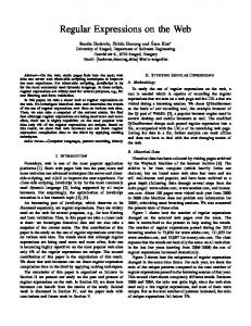
definitions and with the above-mentioned differences, their variants for counter systems are defined unambiguously (see a lengthy presentation of Past LTL for counter systems in [5]). However, we may recall a few definitions on-the-fly if needed. Herein the size of formulae is understood as the number of subformulae. Example. In adjoining figure, we present a flat counter system with two counters and with labeling function l such that l(q3 ) = {p, q} and l(q5 ) = {p}. We would like to characterize the set of configurations c with control state q1 such that there is some infinite run from c for which after some position i, all future even positions j (i.e. i ≡2 j) satisfy that p holds and the first counter is equal to the second counter. start

q1

⊤, (0, −2) ⊤, (0, 0) q4

⊤, (0, 0)

⊤, (0, 0)

q2

⊤, (−3, 0)

⊤, (0, 0)

q3

g′ (x1 , x2 ), (1, 0)

g(x1 , x2 ), (0, 1)

This can be specified in linear µ-calculus using as atomic formulae either propositional variables or atomic guards. The corresponding formula in linear µ-calculus is: µz1 .(X(νz2 .(p ∧ (x1 − x2 = 0) ∧ XXz2 ) ∨ Xz1 ). Clearly, such a position i occurs in any run after reaching the control state q3 with the same value for both counters. Hence, the configurations hq1 , vi satisfying these properties have counter values v ∈ N2 verifying the Presburger formula below:

q5

∃ y (((x1 = 3y + x2 ) ∧ (∀ y′ g(x2 + y′ , x2 + y′ ) ∧ g′ (x2 + y′ , x2 + y′ + 1)))∨ ((x2 = 2y + x1 ) ∧ (∀ y′ g(x1 + y′ , x1 + y′ ) ∧ g′ (x1 + y′ , x1 + y′ + 1)))) In the paper, we shall establish how to compute systematically such formulae (even without universal quantifications) for different specification languages.

3

Constrained Path Schemas

In [5] we introduced minimal path schemas for flat counter systems. Now, we introduce constrained path schemas that are more abstract than path schemas. A constrained path schema cps is a pair hp1 (l1 )∗ · · · pk−1 (lk−1 )∗ pk (lk )ω , φ(x1 , . . . , xk−1 )i where the first component is an ω-regular expression over a constrained alphabet hat, agn , Σi with pi , li ’s in Σ∗ , and φ(x1 , . . . , xk−1 ) ∈ G(Ck−1 ). def Each constrained path schema defines a language L(cps) ⊆ Σω given by L(cps) = nk−1 ω n1 pk (lk ) : φ(n1 , . . . , nk−1 ) holds true}. The size of {p1 (l1 ) · · · pk−1 (lk−1 ) cps, written size(cps), is equal to 2k + len(p1 l1 · · · pk−1 lk−1 pk lk ) + size(φ(x1 , . . . , xk−1 )). Observe that in general constrained path schemas are defined under constrained alphabet and so will the associated specifications unless stated otherwise. Let us consider below the three decision problems on constrained path schemas that are useful in the rest of the paper. Consistency problem checks whether L(cps) is non-empty. It amounts to verify the satisfiability status of the second component. Let us recall the result below. 5

Theorem 1. [22] There are polynomials pol1 (·), pol2 (·) and pol3 (·) such that for every guard g, say in G(Cn ), of size N , we have (I) there exist B ⊆ [0, 2pol1 (N ) ]n and P1 , . . . , Pα ∈ [0, 2pol1 (N ) ]n with α ≤ 2pol2 (N ) such that for every y ∈ Nn , y |= g iff there are b ∈ B and a ∈ Nα such that y = b + a[1]P1 + · · · + a[α]Pα ; (II) if g is satisfiable, then there is y ∈ [0, 2pol3 (N ) ]n s.t. y |= g. Consequently, the consistency problem is NP-complete (the hardness being obtained by reducing SAT). The intersection non-emptiness problem, clearly related to model-checking problem, takes as input a constrained path schema cps and a specification A ∈ L and asks whether L(cps) ∩ L(A) 6= ∅. Typically, for several specification languages L, we establish the existence of a computable map fL (at most exponential) such that whenever L(cps) ∩ L(A) 6= ∅ there is p1 (l1 )n1 · · · pk−1 (lk−1 )nk−1 pk (lk )ω belonging to the intersection and for which each ni is bounded by fL (A, cps). This motivates the introduction of the membership problem for L that takes as input a constrained path schema cps, a specification A ∈ L and n1 , . . . , nk−1 ∈ N and checks whether p1 (l1 )n1 · · · pk−1 (lk−1 )nk−1 pk (lk )ω ∈ L(A). Here the ni ’s are understood to be encoded in binary and we do not require them to satisfy the constraint of the path schema. Since constrained path schemas are abstractions of path schemas used in [5], from this work we can show that runs from flat counter systems can be represented by a finite set of constrained path schemas as stated below. Theorem 2. Let at be a finite set of atomic propositions, agn be a finite set of atomic guards from G(Cn ), S be a flat counter system whose atomic propositions and atomic guards are from at ∪ agn and c0 = hq0 , v0 i be an initial configuration. One can construct in exponential time a set X of constrained path schemas s.t.: (I) Each constrained path schema cps in X has an alphabet of the form hat, agn , Σi (Σ may vary) and cps is of polynomial size. (II) Checking whether a constrained path schema belongs to X can be done in polynomial time. (III) For every run ρ from c0 , there is a constrained path schema cps in X and w ∈ L(cps) such that ρ |= w. (IV) For every constrained path schema cps in X and for every w ∈ L(cps), there is a run ρ from c0 such that ρ |= w. In order to take advantage of Theorem 2 for the verification of flat counter systems, we need to introduce an additional property: L has the nice subalphabet property iff for all specifications A ∈ L over hat, agn , Σi and for all constrained alphabets hat, agn , Σ′ i, one can build a specification A′ over hat, agn , Σ′ i in polynomial time in the sizes of A and hat, agn , Σ′ i such that L(A) ∩ (Σ′ )ω = L(A′ ). We need this property to build from A and a constraint path schema over hat, agn , Σ′ i, the specification A′ . This property will also be used to transform a specification over hat, agn , Σi into a specification over the finite alphabet Σ′ . Lemma 3. BA, ABA, µTL, ETL, Past LTL have the nice subalphabet property. The abstract Algorithm 1 which performs the following steps (1) to (3) takes as input S, a configuration c0 and A ∈ L and solves MC(L, CF S): (1) Guess cps over hat, agn , Σ′ i in X; (2) Build A′ such that L(A) ∩ (Σ′ )ω = L(A′ ); (3) Return 6

L(cps) ∩ L(A′ ) 6= ∅. Thanks to Theorem 2, the first guess can be performed in polynomial time and with the nice subalphabet property, we can build A′ in polynomial time too. This allows us to conclude the following lemma which is a consequence of the correctness of the above algorithm (Appendix C). Lemma 4. If L has the nice subalphabet property and its intersection nonemptiness problem is in NP[resp. PSpace], then MC(L, CF S) is in NP[resp. PSpace] We know that the membership problem for Past LTL is in PTime and the intersection non-emptiness problem is in NP (as a consequence of [5, Theorem 3]). By Lemma 4, we are able to conclude the main result from [5]: MC(PastLTL, CF S) is in NP. This is not surprising at all since in this paper we present a general method for different specification languages that rests on Theorem 2 (a consequence of technical developments from [5]).

4

Taming First-Order Logic and Flat Counter Systems

In this section, we consider first-order logic as a specification language. By Kamp’s Theorem, first-order logic has the same expressive power as Past LTL and hence model-checking first-order logic over flat counter systems is decidable too [5]. However this does not provide us an optimal upper bound for the model-checking problem. In fact, it is known that the satisfiability problem for first-order logic formulae is non-elementary and consequently the translation into Past LTL leads to a significant blow-up in the size of the formula. 4.1

First-Order Logic in a Nutshell

For defining first-order logic formulae, we consider a countably infinite set of variables Z and a finite (unconstrained) alphabet Σ. The syntax of first-order logic over atomic propositions FOΣ is then given by the following grammar: φ ::= a(z) | S(z, z′ ) | z < z′ | z = z′ | ¬φ | φ ∧ φ′ | ∃z φ(z) where a ∈ Σ and z, z′ ∈ Z. For a formula φ, we will denote by f ree(φ) its set of free variables defined as usual. A formula with no free variable is called a sentence. As usual, we define the quantifier height qh(φ) of a formula φ as the maximum nesting depth of the operators ∃ in φ. Models for FOΣ are ω-words over the alphabet Σ and variables are interpreted by positions in the word. A position assignment is a partial function f : Z → N. Given a model w ∈ Σω , a FOΣ formula φ and a position assignment f such that f (z) ∈ N for every variable z ∈ f ree(φ), the satisfaction relation |=f is defined as usual. Given a FOΣ sentence φ, we write w |= φ when w |=f φ for an arbitrary position assignment f . The language of ω-words w over Σ associated to a sentence φ is then L(φ) = {w ∈ Σω | w |= φ}. For n ∈ N, we define the equivalence relation ≈n between ω-words over Σ as: w ≈n w′ when for every sentence φ with qh(φ) ≤ n, w |= φ iff w′ |= φ. 7

FO on CS. FO formulae interpreted over infinite runs of counter systems are defined as FO formulae over a finite alphabet except that atomic formulae of the form a(z) are replaced by atomic formulae of the form p(z) or g(z) where p is an atomic formula or g is an atomic guard from G(Cn ). Hence, a formula φ built over atomic formulae from a finite set at of atomic propositions and from a finite set agn of atomic guards from G(Cn ) defines a specification for the constrained alphabet hat, atn , 2at∪agn i. Note that the alphabet can be ofWexponential size in the size of φ and p(z) actually corresponds to a disjunction p∈a a(z). Lemma 5. FO has the nice subalphabet property. We have taken time to properly define first-order logic for counter systems (whose models are runs of counter systems, see also Section 2.2) but below, we will mainly operate with FOΣ over a standard (unconstrained) alphabet. Let us state our first result about FOΣ which allows us to bound the number of times each loop is taken in a constrained path schema in order to satisfy a formula. We provide a stuttering theorem equivalent for F OΣ formulas as is done in [5] for PLTL and in [13] for LTL. The lengthy proof of Theorem 6 uses EhrenfeuchFraïssé game (Appendix E). Theorem 6 (Stuttering Theorem). Let w = w1 sM w2 , w′ = w1 sM+1 w2 ∈ Σω such that N ≥ 1, M > 2N +1 and s ∈ Σ+ . Then w ≈N w′ . 4.2

Model-Checking Flat Counter Systems with FO

Let us characterize the complexity of MC(FO, CF S). First, we will state the complexity of the intersection non-emptiness problem. Given a constrained path schema cps and a FO sentence ψ, Theorem 1 provides two polynomials pol1 and pol2 to represent succinctly the solutions of the guard in cps. Theorem 6 allows us to bound the number of times loops are visited. Consequently, we can compute a value fFO (ψ, cps) exponential in the size of ψ and cps, as explained earlier, which allows us to find a witness for the intersection non-emptiness problem where each loop is taken a number of times smaller than fFO (ψ, cps). Lemma 7. Let cps be a constrained path schema and ψ be a FOΣ sentence. Then L(cps) ∩ L(ψ) is non-empty iff there is an ω-word in L(cps) ∩ L(ψ) in which each loop is taken at most 2(qh(ψ)+2)+pol1 (size(cps))+pol2 (size(cps)) times. Hence fFO (ψ, cps) has the value 2(qh(ψ)+2)+(pol1 +pol2 )(size(cps)) . Furthermore checking whether L(cps) ∩ L(ψ) is non-empty amounts to guess some n ∈ [0, 2(qh(ψ)+2)+pol1 (size(cps))+pol2 (size(cps)) ]k−1 and verify whether w = p1 (l1 )n[1] · · · pk−1 (lk−1 )n[k−1] pk (lk )ω ∈ L(cps) ∩ L(ψ). Checking if w ∈ L(cps) can be done in polynomial time in (qh(ψ) + 2) + pol1 (size(cps)) + pol2 (size(cps)) (and therefore in polynomial time in size(ψ) + size(cps)) since this amounts to verify whether n |= φ. Checking whether w ∈ L(ψ) can be done in exponential space in size(ψ) + size(cps) by using [17, Proposition 4.2]. Hence, this leads to a nondeterministic exponential space decision procedure for the intersection nonemptiness problem but it is possible to get down to nondeterministic polynomial 8

space using the succinct representation of constrained path schema as stated by Lemma 8 below for which the lower bound is deduced by the fact that modelchecking ultimately periodic words with first-order logic is PSpace-hard [17]. Lemma 8. Membership problem with FOΣ is PSpace-complete. Note that the membership problem for FO is for unconstrained alphabet, but due to the nice subalphabet property of FO, the same holds for constrained alphabet since given a FO formula over hat, agn , Σi, we can build in polynomial time a FO formula over hat, agn , Σ′ i from which we can build also in polynomial time a formula of FOΣ′ (where Σ′ is for instance the alphabet labeling a constrained path schema). We can now state the main results concerning FO. Theorem 9. (I) The intersection non-emptiness problem with FO is PSpacecomplete. (II) MC(FO, CF S) is PSpace-complete. (III) Model-checking flat Kripke structures with FO is PSpace-complete. Proof. (I) is a consequence of Lemma 7 and Lemma 8. We obtain (II) from (I) by applying Lemma 4 and Lemma 5. (III) is obtained by observing that flat Kripke structures form a subclass of flat counter systems. To obtain the lower bound, we use that model-checking ultimately periodic words with first-order logic is PSpace-hard [17]. ⊓ ⊔

5

Taming Linear µ-calculus and Other Languages

We now consider several specification languages defining ω-regular properties on atomic propositions and arithmetical constraints. First, we deal with BA by establishing Theorem 10 and then deduce results for ABA, ETL and µTL. Theorem 10. Let B = hQ, Σ, q0 , ∆, F i be a Büchi automaton (with standard definition) and cps = hp1 (l1 )∗ · · · pk−1 (lk−1 )∗ pk (lk )ω , φ(x1 , . . . , xk−1 )i be a constrained path schema over Σ. We have L(cps) ∩ L(B) 6= ∅ iff there exists y ∈ [0, 2pol1 (size(cps)) +2.card(Q)k ×2pol1 (size(cps))+pol2 (size(cps)) ]k−1 such that p1 (l1 )y[1] . . . pk−1 (lk−1 )y[k−1] pk lkω ∈ L(B) ∩ L(cps) (pol1 and pol2 are from Theorem 1). Theorem 10 can be viewed as a pumping lemma involving an automaton and semilinear sets. Thanks to it we obtain an exponential bound for the map fBA so that fBA (B, cps) = 2pol1 (size(cps)) +2.card(Q)size(cps) ×2pol1 (size(cps))+pol 2 (size(cps)) . So checking L(cps) ∩ L(B) 6= ∅ amounts to guess some n ∈ [0, 2pol1 (size(cps)) + 2.card(Q)size(cps) ×2pol1 (size(cps))+pol2 (size(cps)) ]k−1 and to verify whether the word w = p1 (l1 )n[1] · · · pk−1 (lk−1 )n[k−1] pk (lk )ω ∈ L(cps) ∩ L(B). Checking whether w ∈ L(cps) can be done in polynomial time in size(B) + size(cps) since this amounts to check n |= φ. Checking whether w ∈ L(B) can be also done in polynomial time by using the results from [17]. Indeed, w can be encoded in polynomial time as a pair of straight-line programs and by [17, Corollary 5.4] this can be done in polynomial time. So, the membership problem for Büchi automata is in PTime. By using that BA has the nice subalphabet property and that we can create a polynomial size Büchi automata from a given BA specification and cps, we get the following result. 9

Lemma 11. The intersection non-emptiness problem with BA is NP-complete. Now, by Lemma 3, Lemma 4 and Lemma 11, we get the result below for which the lower bound is obtained from an easy reduction of SAT. Theorem 12. MC(BA, CF S) is NP-complete. We are now ready to deal with ABA, ETL and linear µ-calculus. A language L has the nice BA property iff for every specification A from L, we can build a Büchi automaton BA such that L(A) = L(BA ), each state of BA is of polynomial size, it can be checked if a state is initial [resp. accepting] in polynomial space and the transition relation can be decided in polynomial space too. So, given a language L having the nice BA property, a constrained path schema cps and a specification in A ∈ L, if L(cps) ∩ L(A) is non-empty, then there is an ωword in L(cps) ∩ L(A) such that each loop is taken at most a number of times bounded by fBA (BA , cps). So fL (A, cps) is obviously bounded by fBA (BA , cps). Hence, checking whether L(cps)∩L(A) is non-empty amounts to guess some n ∈ [0, fL (A, cps)]k−1 and check whether w = p1 (l1 )n[1] · · · pk−1 (lk−1 )n[k−1] pk (lk )ω ∈ L(cps) ∩ L(A). Checking whether w ∈ L(cps) can be done in polynomial time in size(A) + size(cps) since this amounts to check n |= φ. Checking whether w ∈ L(A) can be done in nondeterministic polynomial space by reading w while guessing an accepting run for BA . Actually, one guesses a state q from BA and check whether the prefix p1 (l1 )n[1] · · · pk−1 (lk−1 )n[k−1] pk can reach it and then q in which q is an initial nonemptiness between (lk )ω and the Büchi automaton BA state is checked. Again, this can be done in nondeterministic polynomial space thanks to the nice BA property. We obtain the lemma below. Lemma 13. Membership problem and intersection non-emptiness problem for L having the nice BA property are in PSpace. Let us recall consequences of results from the literature. ETL has the nice BA property by [26], linear µ-calculus has the nice BA property by [25] and ABA has the nice BA property by [20]. Note that the results for ETL and ABA can be also obtained thanks to translations into linear µ-calculus. By Lemma 13, Lemma 4 and the above-mentioned results, we obtain the following results. Theorem 14. MC(ABA, CF S), MC(ETL, CF S) and MC(µTL, CF S) are in PSpace. Note that for obtaining the PSpace upper bound, we use the same procedure for all the logics. Using that the emptiness problem for finite alternating automata over a single letter alphabet is PSpace-hard [9], we are also able to get lower bounds. Theorem 15. (I) The intersection non-emptiness problem for ABA [resp. µTL] is PSpace-hard. (II) MC(ABA, CF S) and MC(µTL, CF S) are PSpace-hard. According to the proof of Theorem 15 (Appendix K), PSpace-hardness already holds for a fixed Kripke structure, that is actually a simple path schema. 10

Hence, for linear µ-caluclus, there is a complexity gap between model-checking unconstrained path schemas with two loops (in UP∩co-UP [10]) and modelchecking unconstrained path schemas (Kripke structures) made of a single loop, which is in contrast to Past LTL for which model-checking unconstrained path schemas with a bounded number of loops is in PTime [5, Theorem 9]. As an additional corollary, we can solve the global model-checking problem with existential Presburger formulae. The global model-checking consists in characterizing the set of initial configurations from which there exists a run satisfying a given specification. We knew that Presburger formulae exist for global model-checking [6] for Past LTL (and therefore for FO) but we can conclude that they are structurally simple and we provide an alternative proof. Moreover, the question has been open for µTL since the decidability status of MC(µTL, CF S) has been only resolved in the present work. Corollary 16. Let L be a specification language among FO, BA, ABA, ETL or µTL. Given a flat counter system S, a control state q and a specification A in L, one can effectively build an existential Presburger formula φ(z1 , . . . , zn ) such that for all v ∈ Nn . v |= φ iff there is a run ρ starting at hq, vi verifying ρ |= A.

6

Conclusion

We characterized the complexity of MC(L, CF S) for prominent linear-time specification languages L whose letters are made of atomic propositions and linear constraints. We proved the PSpace-completeness of the problem with linear µcalculus (decidability was open), for alternating Büchi automata and also for FO. When specifications are expressed with Büchi automata, the problem is shown NP-complete. Global model-checking is also possible on flat counter systems with such specification languages. Even though the core of our work relies on small solutions of quantifier-free Presburger formulae, stuttering properties, automata-based approach and on-the-fly algorithms, our approach is designed to be generic. Not only this witnesses the robustness of our method but our complexity characterization justifies further why verification of flat counter systems can be at the core of methods for model-checking counter systems. Our main results are in the table below with useful comparisons (‘Ult. periodic KS’ stands for ultimately periodic Kripke structures namely a path followed by a loop). Flat counter systems

µTL ABA ETL BA FO Past LTL

Kripke struct.

Flat Kripke struct.

Ult. periodic KS

PSpace-C (Thm. 14) PSpace-C [25] PSpace-C (Thm. 14) in UP∩co-UP [18] PSpace-C (Thm. 14) PSpace-C PSpace-C (Thm. 14) in PTime (see e.g. [12, p. 3]) in PSpace (Thm. 14) PSpace-C [23] in PSpace [23] in PTime (see e.g. [21,12]) NP-C (Thm.12) in PTime in PTime in PTime PSpace-C (Thm. 9) Non-el. [24] PSpace-C (Thm. 9) PSpace-C [17] NP-C [5] PSpace-C [23] NP-C [11,5] PTime [14]

References 1. A. Arnold and D. Niwinski. Rudiments of µ-calculus. Elsevier, 2001.

11

2. B. Boigelot. Symbolic methods for exploring infinite state spaces. PhD thesis, Université de Liège, 1998. 3. M. Bozga, R. Iosif, and F. Konecný. Fast acceleration of ultimately periodic relations. In CAV’10, volume 6174 of LNCS, pages 227–242. Springer, 2009. 4. H. Comon and Y. Jurski. Multiple counter automata, safety analysis and PA. In CAV’98, volume 1427 of LNCS, pages 268–279. Springer, 1998. 5. S. Demri, A. Dhar, and A. Sangnier. Taming Past LTL and Flat Counter Systems. In IJCAR’12, volume 7364 of LNAI, pages 179–193. Springer, 2012. See also http://arxiv.org/abs/1205.6584. 6. S. Demri, A. Finkel, V. Goranko, and G. van Drimmelen. Model-checking CTL∗ over flat Presburger counter systems. JANCL, 20(4):313–344, 2010. 7. K. Etessami and T. Wilke. An until hierarchy and other applications of an Ehrenfeucht-Fraïssé game for temporal logic. I&C, 160(1–2):88–108, 2000. 8. A. Finkel and J. Leroux. How to compose Presburger accelerations: Applications to broadcast protocols. In FST&TCS’02, volume 2256 of LNCS, pages 145–156. Springer, 2002. 9. P. Jančar and Z. Sawa. A note on emptiness for alternating finite automata with a one-letter alphabet. IPL, 104(5):164–167, 2007. 10. M. Jurdziński. Deciding the winner in parity games is in UP ∩ co-UP. IPL, 68(3):119–124, 1998. 11. L. Kuhtz and B. Finkbeiner. Weak Kripke structures and LTL. In CONCUR’11, volume 6901 of LNCS, pages 419–433. Springer, 2011. 12. O. Kupferman and M. Vardi. Weak alternating automata are not that weak. ACM Transactions on Computational Logic, 2(3):408–429, 2001. 13. A. Kučera and J. Strejček. The stuttering principle revisited. Acta Informatica, 41(7–8):415–434, 2005. 14. F. Laroussinie, N. Markey, and P. Schnoebelen. Temporal logic with forgettable past. In LICS’02, pages 383–392. IEEE, 2002. 15. J. Leroux and G. Sutre. Flat counter systems are everywhere! In ATVA’05, volume 3707 of LNCS, pages 489–503. Springer, 2005. 16. L. Libkin. Elements of Finite Model Theory. Springer, 2004. 17. N. Markey and P. Schnoebelen. Model checking a path. In CONCUR’03, Marseille, France, volume 2761 of LNCS, pages 251–261. Springer, 2003. 18. N. Markey and P. Schnoebelen. Mu-calculus path checking. IPL, 97(6), 2006. 19. M. Minsky. Computation, Finite and Infinite Machines. Prentice Hall, 1967. 20. S. Miyano and T. Hayashi. Alternating finite automata on ω-words. Theor. Comput. Sci., 32:321–330, 1984. 21. N. Piterman. Extending temporal logic with ω-automata. Master’s thesis, The Weizmann Institute of Science, 2000. 22. L. Pottier. Minimal Solutions of Linear Diophantine Systems: Bounds and Algorithms. In RTA’91, pages 162–173. Springer, 1991. 23. A. Sistla and E. Clarke. The complexity of propositional linear temporal logic. JACM, 32(3):733–749, 1985. 24. L. J. Stockmeyer. The complexity of decision problems in automata and logic. PhD thesis, MIT, 1974. 25. M. Vardi. A temporal fixpoint calculus. In POPL’88, pages 250–259. ACM, 1988. 26. M. Vardi and P. Wolper. Reasoning about infinite computations. I&C, 115, 1994. 27. I. Walukiewicz. Automata and logic, 2001. Lecture notes. 28. P. Wolper. Temporal logic can be more expressive. I&C, 56:72–99, 1983.

12

A

Proof of Theorem 2

Below, we provide the main steps of the proof, details can be found in [5]. Proof. (sketch) Let us explain how to build the set X. 1. Given a flat counter system S and a state q from c, there is at most an exponential number of minimal path schemas starting at q in the sense of [5, Lemma 4]. Let Y1 be this set of minimal path schemas. 2. For each path schema P in Y1 , there is a set of path schemas YP such that the path schemas in YP have no disjunctions in guards and satisfaction of guards can be concluded from the states, see [5, Theorem 14]. Let Y2 be this set of unfolded path schemas and it is of cardinality at most exponential. 3. Following [5, Lemma 12], every path schema from Y2 is equivalent to a constrained path schema. The set X is precisely the set of constrained path schemas obtained from all the unfolded path schemas from Y2 . Completeness of the set X is a consequence of [5, Lemma 12] and [5, Theorem 14(4–6)]. Satisfaction of the size constraints is a consequence of [5, Lemma 12] and [5, Theorem 14(2–3)]. ⊓ ⊔

B

Proof of Lemma 3

Proof. Let A = hQ, E, q0 , F i be a specification in BA. over the alphabet hat, agn , Σi ′ ω and Σ′ ⊆ Σ. The specification A′ = hQ, E ′ , q0 , F i such that L(A′ ) = L(A)∩(Σ ) is W (

ψ

a∈Σ′

ψa )∧ψ

defined as follows: for every q − → q ′ ∈ E, we include in E ′ the edge q −−−−−−−−→ ′ q where ϕa is defined as a conjunction made of positive literals from a and negative literals from (at ∪ agn ) \ a. A similar transformation can be performed with specifications in ABA. Let φ be a formula for L among linear µ-calculus, ETL or Past LTL built over atomic formulae in at ∪ agn and hat, agn , Σ′ i be a constrained alphabet. The formulae φ′ such that W L(φ′ ) = L(φ) ∩ (Σ′ )ω is obtained from φ by replacing every ⊓ ⊔ atomic formula ψ by {a∈Σ′ |ψ∈a} ϕa .

C

Correctness of Algorithm 1

Proof. First assume there exists a run ρ of S starting at c0 such that ρ |= A. By Theorem 2, there is a constrained path schema cps with an alphabet of the form hat, agn , Σ′ i in X and w ∈ L(cps) such that ρ |= w. Consequently we deduce that w ∈ L(A) and that L(cps) ∩ L(A) 6= ∅. Since L(cps) ⊆ (Σ′ )ω and since L(A) ∩ (Σ′ )ω = L(A′ ), we deduce that L(cps) ∩ L(A′ ) 6= ∅. Hence the Algorithm has an accepting run. Now if the Algorithm 1 has an accepting run, we deduce that there exists a constrained path schema cps with an alphabet of the form hat, agn , Σ′ i in X such that there exists a word w in L(cps) ∩ L(A′ ). Using the nice subalphabet 13

property we deduce that w ∈ L(A) and by the last point of Theorem 2, we know that there exists a run ρ from S starting at c0 such that ρ |= w. This allows us to conclude that ρ |= A. ⊓ ⊔

D

Proof of Lemma 5

Proof. Consider a FO formula φ that defines a specification over the constrained alphabet hat, agn , Σi with Σ = 2at∪agn . Consider a subalphabet Σ′ ⊆ Σ. Let φ′′ be the formula obtained from φ by replacing every occurrence of p(z) by W W a(z) and every occurrence of g(z) is replaced by ′ ′ {a∈Σ |g∈a} a(z). It {a∈Σ |p∈a} is easy to see that, by construction, L(φ′′ ) = L(φ′ ) ∩ (Σ)ω ⊓ ⊔

E E.1

EF Games and Proof of Theorem 6 Ehrenfeucht-Fraïssé Games

Ehrenfeucht-Fraïssé (EF) game is a well known technique to determine whether two structures are equivalent with respect to a set of formulae. We recall here the definition of a EF game adapted to our context. Given N ∈ N and two ω-words w, w′ over Σ, the main idea of the corresponding EF game is that two players, the Spoiler and the Duplicator, plays in a turn based manner. The Spoiler begins by choosing a word between w and w′ and a position in this word, then the Duplicator aims at finding a position in the other word which is similar and this during N rounds. At the end, the Duplicator wins if the set of chosen positions respects some isomorphism. We now move to the formal definition of such a game. Let w and w′ be two ω-words over Σ. We define a play as a finite sequence of triples (p1 , a1 , b1 )(p2 , a2 , b2 ) · · · (pi , ai , bi ) in ({0, 1} × N2 )∗ where for each triple the first element describes which word has been chosen by the Spoiler (0 for the word w), then the second element corresponds to the position chosen in w and the third element the position chosen in w′ by the Spoiler or the Duplicator according to the word chosen by the Spoiler. For instance if p1 = 1, this means that at the first turn Spoiler has chosen the position b1 in w′ and Duplicator the position a1 in w. A play of size i ∈ N is called an i-round play (a 0-round play being an empty sequence). A strategy for the Spoiler is a mapping σS : ({0, 1} × N2 )∗ → {0, 1} × N which takes as input a play and outputs 0 or 1 for words w or w′ respectively and a position in the word. Similarly, a strategy for the Duplicator is a mapping σD : ({0, 1} × N2 )∗ × ({0, 1} × N) → N with the difference being that Duplicator takes into account the position played by the Spoiler in the current round. For all i ∈ N, a strategy σS for the Spoiler and a strategy σD for the Duplicator, the i-round play over w and w′ following σS σS ,σD (w, w′ )(p, a, b) and σD is defined inductively as follows: ΠiσS ,σD (w, w′ ) = Πi−1 σS ,σD σS ,σD ′ where if p = 0, (0, a) = σD (Πi−1 (w, w )) and b = σS (Πi−1 (w, w′ ), (0, a)) σS ,σD σS ,σD (w, w′ ), (1, b)). (w, w′ )) and a = σS (Πi−1 and if p = 1, (1, b) = σD (Πi−1 14

For N ∈ N, a N -round play (p1 , a1 , b1 )(p2 , a2 , b2 ) · · · (pN , aN , bN ) over w and w′ is winning for Duplicator iff the following conditions are satisfied for all i, j ∈ [1, N ]: – – – –

ai = aj iff bi = bj , ai + 1 = aj iff bi + 1 = bj , ai < aj iff bi < bj , w(ai ) = w′ (bi ).

A N -round EF game over the ω-words w, w′ , denoted as EFN (w, w′ ), is said to be winning if there exists a strategy σD for Duplicator such that for all σS ,σD (w, w′ ) is winning for Duplicator. We strategies σS of spoiler, the play ΠN ′ ′ write w ≡N w iff the game EFN (w, w ) is winning. Theorem 17 below states that two ω-words, the N -round game is winning iff these two ω-words satisfy the same set of first-order formulae of quantifier height smaller than N . Theorem 17 (EF Theorem, see e.g. [16]). For any two ω-words w, w′ over Σ, w ≡N w′ iff w ≈N w′ . We will use EF games for FOΣ formulae to prove a stuttering theorem which will allow us to bound the number of times each loop needs to be taken in a path schema in order to satisfy a FOΣ formula. Note that in [7], EF games have been introduced for the specific case of LTL specifications here also to show some small model properties. E.2

Stuttering Theorem for FOΣ

In this section, we prove that if in an ω-sequence w, a subword s is repeated consecutively a large number of times, then this ω-word and other ω-words obtained by removing some of the repetitions of s satisfy the same set of FOΣ sentences, this is what we call the stuttering theorem for FOΣ . Such a result will allow us to bound the repetition of iteration of loops in path schema and thus to obtain a model-checking algorithm for the logic FOΣ optimal in complexity. In order to prove the stuttering theorem, we will use EF games. In the sequel we consider a natural N ≥ 1 and two ω-words over Σ of the following form w = w1 sM w2 , w′ = w1 sM+1 w2 ∈ Σω with M > 2N +1 , w1 ∈ Σ∗ , s ∈ Σ+ and w2 ∈ Σω . We will now show that the game EFN (w, w′ ) is winning. The strategy for Duplicator will work as follows: at the i-th round (for i ≤ N ), if the point chosen by the Spoiler is close to another previously chosen position then the Duplicator will choose a point in the other word at the exact same distance from the corresponding position and if the point is far from any other position then in the other word the Duplicator will chose a position also far away from any other position. Before providing a winning strategy for the Duplicator we define some invariants on any i-round play (with i ≤ N ) that will be maintained by the Duplicator’s strategy. In order to define this invariant and the Duplicator’s strategy, let introduce a few notations: 15

– a−3 = b−3 = 0; a−2 = b−2 = len(w1 ); – a−1 = len(w1 sM ) and b−1 = len(w1 sM+1 ); – a0 = b0 = ω. We extend the substraction and addition operations in order to deal with N ∪ {−ω, ω} such that: α − ω = −ω, ω − α = ω and ω + α = ω if α ∈ N (no need to define the other cases for what follows). The relation < on N∪{−ω, ω} is extended in the obvious way. Given a i-round play Πi = (p1 , a1 , b1 )(p2 , a2 , b2 ) · · · (pi , ai , bi ), we say that Πi respects the invariant I iff the following conditions are satisfied for all j, k ∈ [−3, i]: 1. 2. 3. 4. 5. 6.

aj ≤ ak iff bj ≤ bk , | aj − ak |< 2N +1−i len(s) iff | bj − bk |< 2N +1−i len(s), | aj − ak |< 2N +1−i len(s) implies aj − ak = bj − bk , aj ≤ a−2 or bj ≤ b−2 implies bj = aj , aj ≥ a−1 or bj ≥ b−1 implies bj = aj + len(s), a−2 < aj < a−1 or b−2 < bj < b−1 implies | aj − bj |= 0 mod len(s).

First we remark the invariant I is a sufficient condition for a play to be winning as stated by the following lemma. Lemma 18. If a N -round play over w and w′ respects I, then it is a winning play for the Duplicator. Proof. Let (p1 , a1 , b1 )(p2 , a2 , b2 ) · · · (pN , aN , bN ) be a N -round play over w and w′ respecting I. Let i, j ∈ [1, N ]. It is easy to see that satisfaction of I implies that ai = aj iff bi = bj , ai < aj iff bi < bj , and ai + 1 = aj iff bi + 1 = bj . Moreover, Condition I(4–6) obviously guarantees that w(aj ) = w′ (bj ). ⊓ ⊔ Given an (i − 1)-round play Πi−1 = (p1 , a1 , b1 )(p2 , a2 , b2 ) · · · (pi−1 , ai−1 , bi−1 ) and ai ∈ N such that ai 6∈ {a−3 , a−2 , . . . , ai−2 , ai−1 }, we define left (ai ) = max(ak | k ∈ [−3, i − 1] and ak < ai ) and right (ai ) = min(ak | k ∈ [−3, i − 1] and ai < ak ) (i.e. left (ai ) and right (ai ) are the closest neighbor of ai ). We define similarly left (bi ) and right (bi ). We define now a strategy σ ˆD for the Duplicator that respects at each round the invariant I and this no matter what the Spoiler plays. By Lemma 18, we can conclude that this strategy is winning for the Duplicator. Let i ∈ [1, N ] and Πi−1 = (p1 , a1 , b1 )(p2 , a2 , b2 ) · · · (pi−1 , ai−1 , bi−1 ) be a (i − 1)-round play. First, we define bi = σD (Πi−1 , h0, ai i) that is what Duplicator answers if the Spoiler chooses position ai in the ω-word w. We have bi = σ ˆD (Πi−1 , h0, ai i) defined as follows: def

– If ai = aj for some j ∈ [−3, i − 1], then bi = bj ; – Otherwise, let al = left (ai ) and ar = right (ai ): def • If ai − al ≤ ar − ai , we have bi = bl + (ai − al ) def • If ar − ai < ai − al , we have bi = br − (ar − ai ) Similarly we have ai = σ ˆD (Πi−1 , h1, bi i) defined as follows: 16

def

– If bi = bj for some j ∈ [−3, i − 1], then ai = aj ; – Otherwise, let bl = left (bi ) and br = right (bi ): def • If bi − bl ≤ br − bi , we have ai = al + (bi − bl ) def • If br − bi < bi − bl , we have ai = ar − (br − bi ) Lemma 19. For any Spoiler’s strategy σS and for all i ∈ [0, N ], we have that ΠiσS ,ˆσD (w, w′ ) respects I. Proof. The proof proceeds by induction on i. The base case for i = 0 is obvious since the empty play respects I. However, we need to use the fact that M > 2N +1 (otherwise condition I.2 might not hold). Let σS be a Spoiler’s strategy and for every i ∈ [1, N − 1], we assume that σS ,ˆ σD σS ,ˆ σD (w, w′ )) = h0, ai i and let (w, w′ ) respects I. Suppose that σS (Πi−1 Πi−1 σS ,ˆ σD (w, w′ ), h0, ai i). bi = σ ˆD (Πi−1 (1.) Let j, k ∈ [−3, i]. If j, k ∈ [−3, i − 1], then by the induction hypothesis, aj ≤ ak iff bj ≤ bk . Otherwise, let suppose j = i and k 6= i (only remaining interesting case). If ai = aj ′ for some j ′ ∈ [−3, i − 1], then bi = bj ′ and therefore ai ≤ ak iff bi ≤ bk by the induction hypothesis. Otherwise, al < ai < ar and bl < bi < br which entails that ai ≤ ak iff bi ≤ bk . (4.) The case j ∈ [−3, i − 1] is immediate from the induction hypothesis. Now, suppose that a−3 ≤ ai ≤ a−2 . If ai = aj for some j ∈ [−3, i − 1], then bi = bj and a−3 ≤ aj ≤ a−2 . By induction hypothesis, bi = bj = aj = ai . Otherwise, al < ai < ar and al = bl and ar = br by induction hypothesis. Either ai − al ≤ ar − ai or ar − ai < ai − al implies that bi = ai . (5.) The case j ∈ [−3, i − 1] is immediate from the induction hypothesis. Now, suppose that a−1 ≤ ai . If ai = aj for some j ∈ [−3, i − 1], then bi = bj and a−1 ≤ aj . By induction hypothesis, bi = bj = aj +len(s) = ai +len(s). Otherwise, al < ai and bl = al + len(s) by induction hypothesis. Since ar = ω, we have bi = bl + (ai − al ) = ai + len(s). (6.) The case j ∈ [−3, i − 1] is immediate from the induction hypothesis. Now, let us deal with j = i. Satisfaction of (4.) and (5.) implies that a−2 < ai < a−1 iff b−2 < bi < b−1 . Suppose that a−2 < ai < a−1 . So, al < ai < ar and by induction hypothesis | al − bl |= 0 mod len(s) and | ar − br |= 0 mod len(s). If ai − al ≤ ar − ai , then bi = bl + (ai − al ) and | ai − bi |=| al − bl |, whence | ai − bi |= 0 mod len(s). Similarly, if ar − ai < ai − al , then bi = br − (ar − ai ) and | ai − bi |=| ar − br |, whence | ai − bi |= 0 mod len(s). (2.–3.) Let j, k ∈ [−3, i]. If j, k ∈ [−3, i − 1], then by the induction hypothesis, it is easy to verify that – | aj − ak |< 2N +1−i len(s) iff | bj − bk |< 2N +1−i len(s), – | aj − ak |< 2N +1−i len(s) implies aj − ak = bj − bk . Indeed, it is a consequence of the stronger properties below satisfied by induction hypothesis: – | aj − ak |< 2N +2−i len(s) iff | bj − bk |< 2N +2−i len(s), – | aj − ak |< 2N +2−i len(s) implies aj − ak = bj − bk . 17

Otherwise, let suppose j = i and k 6= i (only remaining interesting case). If ai = aj ′ for some j ′ ∈ [−3, i − 1], then by the induction hypothesis, we have – | aj ′ − ak |< 2N +2−i len(s) iff | bj ′ − bk |< 2N +2−i len(s), – | aj ′ − ak |< 2N +2−i len(s) implies aj ′ − ak = bj ′ − bk . Again, this implies that (I) | ai − ak |< 2N +1−i len(s) iff | bi − bk |< 2N +1−i len(s), (II) | ai − ak |< 2N +1−i len(s) implies ai − ak = bi − bk . Now, suppose that there is no j ′ ∈ [−3, i − 1] such that ai = aj ′ . Case 1: ai − al ≤ ar − ai and bi = bl + (ai − al ). Case 1.1: ak ≤ al . – ak = al : | ai − ak |=| bi − bk | and therefore (I)-(II) holds. – ak < al : If | al − ak |≥ 2N +1−i len(s), by induction hypothesis | bl − bk |≥ 2N +1−i len(s) and bk < bl . So, | ai − ak |≥ 2N +1−i len(s) and | bi − bk |≥ 2N +1−i . If | ai − al |≥ 2N +1−i len(s), by definition of bl , | ai − al |=| bi − bl |≥ 2N +1−i len(s) and bk < bl . So, | ai − ak |≥ 2N +1−i len(s) and | bi − bk |≥ 2N +1−i . If | al − ak |≤ 2N +1−i len(s) and | ai − al |≤ 2N +1−i len(s), then by induction hypothesis | bl − bk |=| al − ak |, | ai − al |=| bi − bl |, ak < al < ai and bk < bl < bi . So | ai − ak |=| bi − bk |, whence (I)–(II) holds. Case 1.2: ar ≤ ak . – | ak −ar |≥ 2N +1−i len(s): By induction hypothesis, | bk −br |≥ 2N +1−i len(s). So, | ak −ai |≥ 2N +1−i len(s) and | bk −bi |≥ 2N +1−i len(s) since ai < ar ≤ ak and bi < br ≤ bk . – | ak − ar |≤ 2N +1−i len(s): By induction hypothesis, | bk − br |=| ak − ar |. Case 1.2.1. | ar − al |≤ 2N +2−i len(s). By induction hypothesis, | ar − al |=| br − bl | and therefore | br − bi |=| ar − ai |. Whence, | bk − bi |=| ak − ai | so (I)-(II) holds. Case 1.2.2 | ar − al |≥ 2N +2−i len(s). By induction hypothesis, | br − bl |≥ 2N +2−i len(s). Moreover, since ai −al ≤ ar −ai , ar −ai ≥ 2N +1−i len(s). Since bi −bl = ai −bl , we have br −bi ≥ 2N +1−i len(s) too. So, ak −ai ≥ 2N +1−i len(s) and bk − bi ≥ 2N +1−i len(s), which guarantees (I)–(II). Case 2: ar − ai < ai − al and bi = br − (ar − ai ). Case 2.1: ak ≥ ar . Similar to Case 1.1 by replacing al by ar , bl by br and, by permuting ’’ and ’≤’ by ’≥’ about positions. Case 2.2: ak ≤ al . Similar to Case 1.2 by replacing ar by al , br by bl and, by permuting ’’ and ’≤’ by ’≥’ about positions. ⊓ ⊔ Using Lemma 18 and 19, we deduce that Duplicator has a winning strategy against any strategy of the Spoiler in EFN (w, w′ ), so by Theorem 17, we can conclude Theorem 6 [Stuttering Theorem]. 18

F

Proof of Lemma 7

Proof. Let cps = hp1 (l1 )∗ · · · pk−1 (lk−1 )∗ pk (lk )ω , φ(x1 , . . . , xk−1 )i be a constrained path schema and ψ be a first-order sentence. Suppose that p1 (l1 )n[1] · · · pk−1 (lk−1 )n[k−1] pk (lk )ω ∈ L(cps) ∩ L(ψ). Let B ⊆ [0, 2p1 (size(cps)) ]k−1 and P1 , . . . , Pα ∈ [0, 2p1 (size(cps)) ]k−1 defined for the guard φ following Theorem 1. Since n |= φ, there are b ∈ B and a ∈ Nα such that n = b + a[1]P1 + · · · + a[α]Pα . Let a′ ∈ Nα defined from a such that a′ [i] = a[i] if a[i] ≤ 2qh(ψ)+1 + 1 otherwise a′ [i] = 2qh(ψ)+1 + 1. Note that n′ = b + a′ [1]P1 + · · · + a′ [α]Pα still satisfies φ and for every loop i ∈ [1, k − 1], n[i] > 2qh(ψ)+1 iff ′ ′ n′ [i] > 2qh(ψ)+1 . By Theorem 6, p1 (l1 )n [1] · · · pk−1 (lk−1 )n [k−1] pk (lk )ω ∈ L(ψ). Now, let us bound the values in n′ . – There are at most 2p2 (size(cps)) periods. – Each basis or period has values in [0, 2p1 (size(cps)) ]. – Each period in n′ is taken at most 2qh(ψ)+1 + 1 times. Consequently, each n′ [i] is bounded by 2p1 (size(cps)) + (2qh(ψ)+1 + 1)2p2 (size(cps)) × 2p2 (size(cps)) which is itself bounded by 2(qh(ψ)+2)+p1 (size(cps))+p2 (size(cps)) .

G

⊓ ⊔

Proof of Lemma 8

Proof. We want to show that the membership problem with first-order logic (with unconstrained alphabets) can be solved in polynomial space in size(cps) + size(ψ). Let cps, ψ and n ∈ Nk−1 be an instance of the problem. For i ∈ [1, k−1], def let n′ [i] = min(n[i], 2qh(ψ)+1 + 1). By Theorem 6, the propositions below are equivalent: – p1 (l1 )n[1] · · · pk−1 (lk−1 )n[k−1] pk (lk )ω ∈ L(ψ), ′ ′ – p1 (l1 )n [1] · · · pk−1 (lk−1 )n [k−1] pk (lk )ω ∈ L(ψ). Without any loss of generality, let us assume then that n ∈ [0, 2qh(ψ)+1 + 1]k−1 . Let us decompose w = p1 (l1 )n[1] · · · pk−1 (lk−1 )n[k−1] pk (lk )ω as u · (v)ω where u = p1 (l1 )n[1] · · · pk−1 (lk−1 )n[k−1] pk and v = lk . Note that the length of u is exponential in the size of the instance. We write ψˆ to denote the formula ψ in which every existential quantification is relativized to positions less than len(u)+ len(v) × 2qh(ψ) . This means that every quantification ’∃ x · · · ’ is replaced by ˆ Now, ’∃ x < (len(u)+len(v)×2qh(ψ) ) · · · ’. By [17], we know that w |= ψ iff w |= ψ. checking w |= ψˆ can be done in polynomial space by using a standard first-order model-checking algorithm by restricting ourselves to positions in [0, len(u) + len(v) × 2qh(ψ) ] for existential quantifications. Such positions can be obviously encoded in polynomial space. Moreover, note that given i ∈ [0, len(u) + len(v) × 19

Algorithm 1 FOSAT(cps, n, ψ, f ) 1: 2: 3: 4: 5: 6: 7: 8: 9: 10: 11: 12:

if φ = a(z) then Calculate the f (z)th letter b of w and return a = b. else if ψ is of the form ¬ψ ′ then return not FOSAT(cps, n, ψ ′ , f ) else if ψ = ψ1 ∧ ψ2 then return FOSAT(cps, n, ψ1 , f ) and FOSAT(cps, n, ψ2 , f ). else if ψ is of the form ∃z < m ψ ′ then guess a position k ∈ [0, m − 1]. return FOSAT(cps, n, ψ ′ , f [z 7→ k]). else if φ is of the form R(z, z′ ) for some R ∈ {=, 2.card(Q)k . We would like to find a such that y′ = b + Σi∈[1,j−1] ai .Pi + (aj − a)Pj + Σi∈[j+1,α] ai .Pi and w′ = p1 (l1 )y’[1] . . . pk−1 ′ (lk−1 )y [k−1] pk lkω ∈ L(B) ∩ L(cps). 1. For any a ≤ aj , we have that, w′ with y′ = b + Σi∈[1,j−1] ai .Pi + (aj − a) Pj + Σi∈[j+1,α] ai .Pi , w′ ∈ L(cps). Indeed by selecting any a ∈ [aj , aj − 2.card(Q)k ], we will obtain y′ ∈ [0, 2pol1 (size(cps)) + 2.size(B)k × 2pol1 (size(cps))+pol2 (size(cps)) ]k−1 where w′ ∈ L(cps). 21

2. For showing that there exists a value for a such that y′ ∈ [0, 2pol1 (size(cps)) + 2.size(B)k ×2pol1 (size(cps))+pol2 (size(cps)) ]k−1 and w′ ∈ L(B) we will use Lemma 20. For each m ∈ [1, k − 1], we take rm = (lm )Pj [m] i.e. rm is Pj [m] copies of lm . Note that by our assumption, for each m ∈ [1, k − 1] we can factor w as w = w1m .(rm )am .w2m where am ≥ 2.card(Q)k . Thus, applying Lemma 20, we get that there exist Km ∈ [1, card(Q)] such that for any Nm ∈ [1, card(Q)k−2 ], w′′ = w1m .(rm )am −(Nm ×Km ) .w2m ∈ L(B). For each m ∈ [1, k] we take Nm = K1 × K2 · · · Km−1 × Km+1 · · · Kk−1 which is less than or equal to card(Q)k−2 . It is clear that for each m ∈ [1, k − 1], the number of iteration of rm we reduce is Nm × Km and is same for all m, Nm × Km = K1 × K2 · · · Kk−1 . Combining the result of Lemma 20 for every loop lm , m ∈ [1, k − 1] and taking a = K1 × K2 · · · Kk−1 in y′ we obtain w′ such that w′ ∈ L(B). We can continue the process to obtain y′ ∈ [0, 2pol1 (size(cps)) + 2.size(B)k × 2pol1 (size(cps))+pol2 (size(cps)) ]k−1 and w′ ∈ L(B). ⊓ ⊔

I

Proof of Lemma 11

Proof. Consider any given specification A in BA, a constrained path schema cps.We would first construct the Büchi automaton BA corresponding to A as explained in Section 2.3. Recall, that A in BA has transitions labelled with Boolean combination over at ∪ agn whereas the equivalent BA has transitions labelled with elements of Σ = 2at∪agn . Hence, in effect, BA could have an exponential number of transitions. On the other hand by definition cps is defined over an alphabet Σ′ ⊆ Σ. By Lemma 3, we know that BA has the nice subalphabet property. Hence, we can transform A over Σ to A′ over Σ′ in polynomial time. The Büchi automata BA′ obtained from A′ following the construction in Section 2.3 has transitions labelled by letters from Σ′ . Clearly in this case the number of transitions in BA′ is polynomial in size(cps). We obtain the following equivalences, – using Lemma 3 and the fact that L(cps) ⊆ (Σ′ )ω , L(A)∩L(cps) is non-empty iff w ∈ L(A′ ) ∩ L(cps) is non-empty. – Since, BA′ is obtained from A′ following the construction from Section 2.3, L(BA′ ) ∩ L(cps) is non-empty iff w ∈ L(A′ ) ∩ L(cps) is non-empty. Checking L(BA′ ) ∩ L(cps) amounts to guessing n ∈ fBA (BA′ , cps) and checking for w = p(l1 )n[1] · · · pk−1 (lk−1 )n[k−1] pk lkω , w ∈ L(BA′ ) ∩ L(cps). We know that checking w ∈ L(BA′ ) ∩ L(cps) is in PTime and the construction of BA′ from A takes only polynomial time. Thus, checking L(A) ∩ L(cps) is non-empty can be done in polynomial time. ⊓ ⊔

J

proof of Lemma 13

Proof. First we prove that the membership problem for L having the nice BA property is in PSpace. Let A ∈ L over the constrained alphabet hat, agn , Σi and 22

let w = p1 (l1 )n[1] · · · pk−1 (lk−1 )n[k−1] pk (lk )ω be a word over Σ. We would like to check whether w ∈ L(A) which is equivalent, thanks to the nice BA property, to check whether w ∈ L(BA ). To verify if w ∈ L(BA ), we try to find a “lasso” structure in Büchi automaton. Assume BA = hQ, Σ, ∆, qi , F i. We proceed as follows. First, we guess a state qf ∈ F and a position j ∈ [1, len(lk )]. Then we consider the two finite state automata A1 = hQ, Σ, q0 , ∆, {qf }i and A2 = hQ, Σ, qf , ∆, {qf }i. And our method returns true iff both the following conditions are true: 1. p1 (l1 )y[1] . . . pk−1 (lk−1 )y[k−1] pk lk [1, j] ∈ L(A1 ). 2. L(A2 ) ∩ L(lk [j + 1, len(lk )]lk∗ lk [1, j]) 6= ∅. We will now show the correctness of the above procedure. First let us assume that w = p1 (l1 )y[1] . . . pk−1 (lk−1 )y[k−1] pk lkω ∈ L(BA ). Thus, there is an accepting run ρ ∈ ∆ω for w in BA . According to the Büchi acceptance condition there exists a state qf ∈ F which is visited infinitely often. In w only lk is taken infinitely many times. Thus, lk being of finite size, there exists a position j ∈ lk (j)

[1, len(lk )] such that transitions of the form q −−−→ qf for some q ∈ Q occurs infinitely many times in ρ. Thus, for ρ to be an accepting run, there exists w′ = L(p1 (l1 )y[1] . . . pk−1 (lk−1 )y[k−1] pk lk [1, j]), which has a run in BA from qi to qf and there must exists words w′′ ∈ L(lk [j + 1, len(lk )]lk∗ lk [1, j]) which has a run from qf to qf . Hence we deduce that w′ ∈ L(A1 ) and L(A2 ) ∩ L(lk [j + 1, len(lk )]lk∗ lk [1, j]) 6= ∅. Thus, there exists at least one choice of qf and j, for which both the checks return true and hence the procedure returns true. Now let us assume that the procedure returns true. Thus, there exists qf ∈ F and j ∈ [1, len(lk )] such that w1 = p1 (l1 )y[1] . . . pk−1 (lk−1 )y[k−1] pk lk [1, j] is in L(A1 ) and L(A2 ) ∩ L(lk [j + 1, len(lk )]lk∗ lk [1, j]) 6= ∅. From the second point, we deduce that there exists a word w2 = lk [j + 1, len(lk )]lkn lk [1, j] ∈ L(A2 ) for some n. Consider the word w = w1 .(w2 )ω . First we have directly that w ∈ L(cps). And by construction of A1 and A2 we know that w1 has a run in BA starting from qi to qf and w2 has a run in BA starting from qf to qf . Since qf is an accepting state of BA , we deduce that w ∈ L(BA ). The proof that the above procedure belongs to PSpace is standard and used the nice BA property which allows us to perform the procedure "on-the-fly". First note that for A in L having the nice BA property, the corresponding Büchi automaton BA can be of exponential size in the size of the A, so we cannot construct the transition relation of BA explicitly, instead we do it on-the-fly. We consider the different steps of the procedure and show that they can be done in polynomial space. 1. A1 and A2 are essentially copies of BA and hence their transition relations are also not constructed explicitly. But, by the nice BA property, their states can be represented in polynomial space. 2. Checking p1 (l1 )y[1] . . . pk−1 (lk−1 )y[k−1] pk lk [1, j] ∈ L(A1 ) can be done by simulating A1 on this word. Note that for simulating A1 , at any position we only need to store the previous state and the letter at current position to 23

obtain the next state of A1 . Thus, this can be performed in polynomial space in size(A) and size(cps) + size(y). 3. Checking L(A2 ) ∩ L(lk [j + 1, len(lk )]lk∗ lk [1, j]) 6= ∅ can be done by constructing a finite state automaton Aloop for L(lk [j + 1, len(lk )]lk∗ lk [1, j]) and by checking for reachability of final state in the automaton A2 × Aloop . Note that size(Aloop ) is polynomial, but since size(A2 ) can be of exponential size, size(A2 × Aloop ) can also be of exponential magnitude. However, the graph accessibility problem (GAP) is in NLogSpace, so L(A2 ) ∩ L(Aloop ) 6= ∅ can also be done in nondeterministic polynomial space. Thus, the whole procedure can be completed in nondeterministic polynomial space and by applying Savitch’s theorem, we obtain that for any L, satisfying the nice BA property, the membership problem for L having the nice BA property is in PSpace. Now we will prove that the intersection non-emptiness problem for L having the nice BA property is in PSpace too. Let A in L with the nice BA property and let cps = hp1 (l1 )∗ · · · pk−1 (lk−1 )∗ pk (lk )ω , φ(x1 , . . . , xk−1 )i be a constrained path schema. Thanks to the nice BA property we have that L(cps) ∩ L(A) 6= ∅ iff L(cps) ∩ L(BA ) 6= ∅. Using Theorem 10 we have L(cps) ∩ L(BA ) 6= ∅ iff there exists y ∈ [0, fBA (BA , cps)]k−1 such that p1 (l1 )y[1] . . . pk−1 (lk−1 )y[k−1] pk lkω ∈ L(BA )∩L(cps) where fBA (BA , cps) is equal to 2pol1 (size(cps)) +2.card(Q)size(cps) × 2pol1 (size(cps))+pol 2 (size(cps)) (Q being the set of states of BA whose cardinality is, thanks to the nice BA property, at most exponential in the size of A). Hence our algorithm amounts to guess some y ∈ [0, fBA (BA , cps)]k−1 and check whether w = p1 (l1 )y[1] · · · pk−1 (lk−1 )y[k−1] pk (lk )ω ∈ L(cps)∩L(A). Since the membership problem for A can be done in PSpace and since the y[i] can be encoded in polynomial space in the size of A and CPS, we deduce that the intersection non-emptiness problem for L with the nice BA property is in PSpace. ⊓ ⊔

K

Proof of Theorem 15

Proof. (II) is direct consequence of (I). First, we recall that an alternating finite automaton is a structure of the form A = (Q, Σ, δ, q0 , F ) such that Q and Σ are finite nonempty sets, δ : Q × Σ → B+ (Q) is the transition function (B+ (Q) is the set of positive Boolean formulae built over Q), q0 ∈ Q and F ⊆ Q. The acceptance predicate Acc ⊆ Q × Σ∗ is defined by induction on the length of the second component so that (1) hqf , εi ∈ Acc whenever qf ∈ F and (2) hq, a · wi ∈ Acc iff v |= δ(q, a) where v is the Boolean assignment such that v(q ′ ) = ⊤ iff hq ′ , wi ∈ Acc. We write L(A) to denote the language {w ∈ Σ∗ : hq0 , wi ∈ Acc} and more generally, def L(A, q) = {w ∈ Σ∗ : hq, wi ∈ Acc}. It has been shown in [9] that checking whether an alternating finite automaton A with a singleton alphabet has a nonempty language L(A) is PSpace-hard. Without loss of generality, we can assume that (⋆) q0 6∈ F , (⋆⋆) for every qf ∈ F , δ(qf , a) =⊥ and (⋆ ⋆ ⋆) for every q ∈ Q, 24

δ(q, {a}) 6= ⊤ , assuming that a is the only letter, and still preserves PSpacehardness. Indeed, let A = (Q, {a}, δ, q0 , F ) be an alternating finite automaton and A′ = (Q′ , {a}, δ ′ , q0new , {qfnew }) be its variant such that Q′ = Q⊎{q0new , qfnew }, δ ′ (q0new , a) = q0 , δ ′ (qfnew , a) =⊥ and for every q ∈ Q, δ ′ (q, a) is obtained from δ(q, a) by simultaneously replacing every occurrence of qf ∈ F by (qf ∨ qfnew ). In the case, δ(q, a) = ⊤ with q ∈ Q, δ ′ (q, a) is defined as q ∨ qfnew . It is clear from the construction that A′ follows the conditions of our assumption and L(A′ ) = a · L(A); whence L(A) is non-empty iff L(A′ ) is non-empty. In order to prove the result for ABA, it is sufficient to observe that given an alternating finite automaton A built over the singleton alphabet {a}, one can build in logarithmic space an alternating Büchi automaton A′ over the alphabet {a, b} such that L(A′ ) = L(A)·{b}ω . Roughly speaking, the reduction consists in taking the accepting states of A and in letting them accept {b}ω in A′ . PSpacehardness of the intersection non-emptiness problem for ABA is obtained by noting that L(A) is non-empty iff L(ha∗ · bω , ⊤i) ∩ L(A′ ) 6= ∅. Now, let us deal with µTL. The PSpace-hardness is essentially obtained by reducing nonemptiness problem for alternating finite automata with a singleton alphabet (see e.g. [9]) into the vectorial linear µ-calculus with a fixed simple constrained path schema. Reduction in polynomial-time into linear µ-calculus is then possible when formula sizes are measured in terms of numbers of subformulae. This is a standard type of reduction (see e.g. [27, Section 5.4]); we provide details below not only to be self-contained but also because we need a limited number of resources: no greatest fixed point operator (e.g. no negation of least fixed point operator) and we then use a simple path schema. In the sequel, for ease of presentation, we consider this latter class of alternating finite automata and we present a logarithmic-space reduction into the intersection non-emptiness problem with linear µ-calculus. More precisely, for every alternating finite automaton A built over the singleton alphabet {{p}}, we build a formula φA in the linear µ-calculus (without X−1 and the greatest fixed-point operator ν) such that L(A) is non-empty iff there is {p} · {p}n1 · ∅ω in L(cps) with the constrained path schema cps = h{p} · {p}∗ · ∅ω , ⊤i and {p} · {p}n1 · ∅ω |= φA . In order to define φA , we build first an intermediate formula in the vectorial version of the linear µ-calculus, see e.g. similar developments in [27, Section 5.4], and then we translate it into an equivalent formula in the linear µ-calculus by using the well-known Bekič’s Principle. Let A = (Q, {{p}}, δ, q0, F ) be a alternating finite automaton with a singleton alphabet such that q0 6∈ F , and for every qf ∈ F , δ(qf , {p}) =⊥. We order the states of Q \ F with q1 , . . . , qα such that q1 is the initial state. We define the formulae in the vectorial version of linear µ-calculus ψ10 , . . . , 0 1 i , . . . , ψ1α−1 and such that µ z1 · ψ1α−1 beψα , ψ11 , . . . , ψα−1 , . . . , ψ1i , . . . , ψα−i longs to the (standard) linear µ-calculus. Such formulae will satisfy the following conditions. (I) For all n ≥ 1, {p}n ∈ L(A) iff {p}n · ∅ω |= µhz1 , . . . , zα i hψ10 , . . . , ψα0 i · z1 . j (II) For all j ∈ [0, α − 1], µhz1 , . . . , zα−j i hψ1j , . . . , ψα−j i · z1 is equivalent to j+1 µhz1 , . . . , zα−j−1 i hψ1j+1 , . . . , ψα−j−1 i · z1 . 25

(III) Consequently, for all n ≥ 1, {p}n ∈ L(A) iff {p}n · ∅ω |= µ z1 · ψ1α−1 and we pose φA = µ z1 · ψ1α−1 . Let us define below the formulae: the substitutions are simple and done hierarchically. (init) For every i ∈ [1, α], ψi0 is obtained from δ(qi , {p}) by substituting each qj ∈ Q\F by Xzj and each qf ∈ F by X¬p, and then by taking the conjunction with p. So, ψi0 can be written schematically as p ∧ δ(qi , {p})[qj ← Xzj , qf ← X¬p]. (ind) For every j ∈ [1, α − 1], for every i ∈ [1, α − j], ψij is obtained from ψij−1 j−1 . by substituting every occurrence of zα−j+1 by µzα−j+1 ψα−j+1 Note that µ z1 · ψ1α−1 can be built in logarithmic space in the size of A since formulae are represented as DAGs (their size is the number of subformulae) and for all j ∈ [1, α − 1] and i ∈ [1, α − j], ψij has no free occurrences of zα−j+1 , . . . , zα . It remains to check that (I)–(III) hold. First, observe that (III) is a direct consequence of (I) and (II). By Bekič’s Principle, see e.g. [1, Section 1.4.2], µhz1 , . . . , zj i hϕ1 (z1 , . . . , zj ), . . . , ϕj (z1 , . . . , zj )i · z1 is equivalent to µhz1 , . . . , zj−1 i hϕ1 (z1 , . . . , zj−1 , ϕ′ ), . . . , ϕj−1 (z1 , . . . , zj−1 , ϕ′ )i · z1 where ϕ′ = µzj ϕj (z1 , . . . , zj ). Note that the substitution performed to build the formula follows exactly the same principle. For every j ∈ [1, α − 1], we obtain j j−1 j−1 hψ1j , . . . , ψα−j i by replacing zα−j+1 by µzα−j+1 ψα−j+1 in hψ1j−1 , . . . , ψα−j+1 i. Thus by Bekič’s Principle, j j+1 µhz1 , . . . , zα−j i hψ1j , . . . , ψα−j i · z1 ⇔ µhz1 , . . . , zα−j−1 i hψ1j+1 , . . . , ψα−j−1 i · z1

is valid for all j ∈ [0, α − 1]. It remains to verify that (I) holds true. In vectorial linear µ-calculus, formulae with outermost fixed-point operators are of the form µhz1 , . . . , zβ ihφ1 , . . . , φβ i · zj with j ∈ [1, β]. Whereas fixed points in linear µ-calculus are considered for monotone functions over the complete lattice h2N , ⊆i, fixed points in vectorial linear µ-calculus are considered for monotone functions over the complete lattice h(2N )β , ⊆i, where hY1 , . . . , Yβ i ⊆ hY1′ , . . . , Yβ′ i iff for every i ∈ [1, β], we have Yi ⊆ Yi′ . So, the satisfaction relation is defined as follows. Given a model σ ∈ (2AT )ω , σ, i |=f µhz1 , . . . , zβ ihφ1 , . . . , φβ i·zj (assuming that the variables zk occurs positively in the φl ’s) iff i ∈ Zjµ where hZ1µ , . . . , Zβµ i is the least fixed point of the monotone function Ff,σ : (2N )β → (2N )β defined by Ff,σ (Y1 , . . . , Yβ ) = hY1′ , . . . , Yβ′ i where Yl′ = {i′ ∈ N : σ, i′ |=f [z1 ←Y1 ,...,zβ ←Yβ ] φl } def

It is well-known that the least fixed point hZ1µ , . . . , Zβµ i can be obtained by an iterative process: hZ10 , . . . , Zβ0 i = h∅, . . . , ∅i, hZ1i+1 , . . . , Zβi+1 i = Ff,σ (Z1i , . . . , Zβi ) S for all i ≥ 0 and, hZ1µ , . . . , Zβµ i = i hZ1i , . . . , Zβi i. def

def

26

Let σn be the model {p}n ·∅ω with n > 0, f∅ be the constant assignment equal to ∅ everywhere and Ff∅ ,σn be the monotone function Ff∅ ,σn : (2N )α → (2N )α defined from µhz1 , . . . , zα i hψ10 , . . . , ψα0 i · z1 . Let us show by induction that for every i ∈ [1, n], the ith iterated tuple hZ1i , . . . , Zαi i verifies that for every l ∈ [1, α], u ∈ Zli iff u ∈ [n − i, n − 1] and {p}n−u ∈ L(A, ql ). Base Case: i = 1. The propositions below are equivalent (l ∈ [1, α]): – u ∈ Zl1 , – σn , u |=f∅ [z1 ←∅,...,zα ←∅] ψl0 (by definition of Ff∅ ,σn ), – σn , u |=f∅ [z1 ←∅,...,zα ←∅] p ∧ δ(qi , {p})[qj ← Xzj , qf ← X¬p] (by definition of ψl0 ), – σn , u |= p ∧ δ(ql , {p})[qj ←⊥, qf ← X¬p] (by definition of |=), – σn , u |= p and there is a Boolean valuation v : Q → {⊥, ⊤} such that for every q ∈ (Q \ F ), we have v(q) =⊥ and v |= δ(ql , {p}), – σn , u |= p, σn , u + 1 |= ¬p and hql , {p}i ∈ Acc (by definition of Acc and by assumption (⋆ ⋆ ⋆)), – u = n − 1 and {p}n−u ∈ L(A, ql ) (by definition of σn and L(A, ql )). Before proving the induction, we observe that we can also show by induction, that for all l ∈ [1, α] and i, Zli ⊆ [n − i, n − 1] (†). Induction Step: Now let us assume that for some i ∈ [1, n], the ith iterated tuple hZ1i , . . . , Zαi i verifies that for every l ∈ [1, α], u ∈ Zli iff u ∈ [n − i, n − 1] and {p}n−u ∈ L(A, ql ). We will show that the same holds true for (i + 1)th iteration hZ1i+1 , . . . , Zαi+1 i. Since Zli ⊆ Zli+1 (monotonicity), for every u ∈ Zli+1 ∩ Zli , we have u ∈ [n − i − 1, n − 1] and {p}n−u ∈ L(A, ql ) (since [n − i, n − 1] ⊆ [n−i−1, n−1]). Similarly, if u ∈ [n−i, n−1] and {p}n−u ∈ L(A, ql ), then u ∈ Zli by induction hypothesis and therefore u ∈ Zli+1 . Hence, it remains to show that u ∈ (Zli+1 \ Zli ) iff u = n − i − 1 and {p}n−u ∈ L(A, ql ) (i.e. {p}i+1 ∈ L(A, ql )). By (†), it is sufficient to show that (n − i − 1) ∈ Zli+1 iff {p}i+1 ∈ L(A, ql ). The propositions below are equivalent (l ∈ [1, α], i ≥ 1, n − i − 1 ≥ 0): – (n − i − 1) ∈ Zli+1 , ), – σn , n − i − 1 |=f∅ [z1 ←Z1i ,...,zα ←Z1i ] ψl0 (by definition of Ffi+1 ∅ ,σn – σn , n − i − 1 |=f∅ [z1 ←Z1i ,...,zα ←Z1i ] p ∧ δ(qi , {p})[qj ← Xzj , qf ← X¬p] (by definition of ψl0 ), – σn , n − i − 1 |= p and there is a Boolean valuation v : Q → {⊥, ⊤} such that 1. for every ql′ ∈ (Q \ F ), we have v(ql′ ) = ⊤ iff n − i ∈ Zli′ , 2. for every qf ∈ F , v(qf ) =⊥, v |= δ(ql , {p}) (by definition of |= and i ≥ 1), – there is v : Q → {⊥, ⊤} such that 1. for every ql′ ∈ (Q \ F ), we have v(ql′ ) = ⊤ iff n − i ∈ [n − i, n − 1] and hql′ , {p}i i ∈ Acc, 2. for every qf ∈ F , v(qf ) =⊥, and v |= δ(ql , {p}) (by induction hypothesis and since n − i − 1 ∈ [0, n − 1]), – there is v : Q → {⊥, ⊤} such that 1. for every ql′ ∈ (Q \ F ), we have v(ql′ ) = ⊤ iff hql′ , {p}i i ∈ Acc, 27

2. for every qf ∈ F , v(qf ) =⊥ and v |= δ(ql , {p}) (by propositional reasoning), – there is v : Q → {⊥, ⊤} such that 1. for every ql′ ∈ (Q \ F ), we have v(ql′ ) = ⊤ iff hql′ , {p}i i ∈ Acc, 2. for every qf ∈ F , v(qf ) = ⊤ iff hqf , {p}i i ∈ Acc, and v |= δ(ql , {p}) (since i ≥ 1, δ(qf , {p}) =⊥ and hqf , {p}i i 6∈ Acc), – hql , {p}i+1 i ∈ Acc (by definition of Acc), – {p}i+1 ∈ L(A, ql ). Thus, for every i ∈ [1, n], the ith iterated tuple hZ1i , . . . , Zαi i verifies that for every l ∈ [1, α], u ∈ Zli iff u ∈ [n − i, n − 1] and {p}n−u ∈ L(A, ql ). So, {p}n ∈ L(A) iff 0 ∈ Z1n . Since hZ1µ , . . . , Zαµ i is precisely equal to hZ1n , . . . , Zαn i because of the simple structure of σn (see (†), we conclude that {p}n ∈ L(A) iff σn , 0 |= µhz1 , . . . , zα i hψ10 , . . . , ψα0 i · z1 , whence (I) holds. From (III), we conclude that L(A) is non-empty iff there is {p} · {p}n1 · ∅ω in L(cps) with cps = h{p} · {p}∗ · ∅ω , ⊤i such that {p} · {p}n1 · ∅ω |= φA . Since cps and φA can be computed in logarithmic space in the size of A, this provides a reduction from the nonemptiness problem for alternating finite automata with a singleton alphabet to the intersection non-emptiness problem with linear µcalculus. Hence, the intersection non-emptiness problem is PSpace-hard (we use only a fixed constrained path schema and a formula without past-time operators and without greatest fixed-point operator). ⊓ ⊔

L

Proof of Corollary 16

Proof. The proof takes advantage of a variant of Theorem 2 (whose proof is also based on developments from [5]) in which initial counter values are replaced by variables. Below, we prove the results for BA, which immediately leads to a similar result for ABA, ETL and µTL. Let S be a flat counter system of dimension n built over atomic constraints in at ∪ agn , q be a control state and A be a specification in BA (i.e. a Büchi automaton whose underlying constrained alphabet is hat, agn , Σi). A parameterized constraint path schema (PCPS) is defined as a constrained path schema except that the second argument (a guard) has also the free variables z1 , . . . ,zn dedicated to the initial counter values. Remember that a constrained path schema has already a constraint about the number of times loops are visited. In its parameterized version, this constraint expresses also a requirement on the initial counter values. Following the proof of Theorem 2, one can construct in exponential time a set X of parameterized constrained path schemas such that: – Each parameterized constrained path schema pcps in X has an alphabet of the form hat, agn , Σ′ i (Σ′ may vary) and pcps is of polynomial size. – Checking whether a parameterized constrained path schema belongs to X can be done in polynomial time. 28

– For every run ρ from hq, vi, there is a parameterized constrained path schema pcps and w ∈ L(pcps[v]) such that ρ |= w where pcps[v] is the contrained path obtained from pcps by replacing the variables z1 , . . . ,zn by the counter values from v. – For every parameterized constrained path schema pcps, for every counter values v, for every w ∈ L(pcps[v]), there is a run ρ from hq, vi such that ρ |= w. The existential Presburger formula φ(z1 , . . . , zn ) has the form below _ _ (∃ y1 , . . . , yM ∃ x1 , . . . , xk−1 pcps=h·,ψi∈X qinit ,q,(lk )ω ∈L(A′q )

ψqinit ,q (y1 , . . . , yM ) ∧ (y1 = α10 + α11 x1 + · · · + α1k−1 xk−1 ) ∧ · · · M M . . . ∧ (yM = αM 0 + α1 x1 + · · · + αk−1 xk−1 ) ∧ ψ(x1 , . . . , xk−1 , z1 , . . . , zn ))

where 1. hat, agn , Σ′ i is the alphabet of pcps, M = card(Σ′ ) and by the nice subalphabet property, there is a specification A′ such that L(A′ ) = L(A) ∩ (Σ′ )ω . 2. qinit is an initial state of A′ and q is a state of A′ . 3. ψqinit ,q (y1 , . . . , yM ) is the quantifier-free Presburger formula for the Parikh image of finite words over the alphabet Σ′ accepted by A′ (viewed as a finitestate automaton) with initial state qinit and final state q. ψqinit ,q (y1 , . . . , yM ) is of polynomial size in the size of Büchi automaton. 4. pcps = hp1 (l1 )∗ · · · pk−1 (lk−1 )∗ pk (lk )ω , ψ(x1 , . . . , xk−1 , z1 , . . . , zn )i. M 5. For each letter aj , we write αM 0 , . . . , αk−1 to denote the natural numbers such that if each loop i in pcps is taken xi times, then the letter aj is visited αj0 + αj1 x1 + · · · + αjk−1 xk−1 times along p1 (l1 )∗ · · · pk−1 (lk−1 )∗ pk . Those coefficients can be easily computed from p1 (l1 )∗ · · · pk−1 (lk−1 )∗ pk (for instance αj1 is the number of times the letter aj is present in the first loop). 6. Finally, observe that checking whether (lk )ω ∈ L(A′q ) where A′q is defined as the specification A′ in which the unique initial state is q, amounts to perform a nonemptiness test between two Büchi automata. FO admits a similar proof but it is based on Theorem 6 (actually the proof is much simpler because the number of times loops can be visited depends essentially on a threshold value). For FO, it is sufficient to consider the formula below: _ _ pcps=hp1 (l1 )∗ ···pk−1 (lk−1 )∗ pk (lk )ω ,ψi∈X y s.t. p1 ly[1] p2 ly[2] ...ly[k−1] pk lω |=A′ 1 2 k−1 k

∃ y1 · · · yk−1 ψ(y1 , . . . , yk−1 , z1 , . . . , zn ) ∧ ψ1 ∧ · · · ∧ ψk−1 where 1. pcps = hp1 (l1 )∗ · · · pk−1 (lk−1 )∗ pk (lk )ω , ψ(x1 , . . . , xk−1 , z1 , . . . , zn )i, 29

2. hat, agn , Σ′ i is the alphabet of pcps and by the nice subalphabet property, there is a specification A′ such that L(A′ ) = L(A) ∩ (Σ′ )ω . ′ 3. the third generalized disjunction deals with y ∈ [0, 2size(A )+1 + 1]k−1 . ′ def def 4. For i ∈ [1, k − 1], ψi = (y1 = α) if y[i] < 2size(A )+1 + 1 otherwise ψi = (yi ≥ size(A′ )+1 2 + 1. ⊓ ⊔

30