classic GoF book [9] on both structural features [2] and be- havioral features [5]. ..... Class Adapter pattern has the static condition Adapter â. ââ³ Adaptee instead ...
On the Composition of Design Patterns Ian Bayley and Hong Zhu School of Technology, Oxford Brookes University, Oxford OX33 1HX, UK (ibayley � hzhu)@brookes.ac.uk Abstract Design patterns are usually applied in a composed form with each other. It is crucial to be able to formally reason about how patterns can be composed and to prove the properties of composed patterns. Based on our previous work on formal specification of design patterns and formal reasoning about their properties, this paper focuses on the composition of design patterns. A notion of composition of patterns with respect to overlaps is formally defined based on two operations on design patterns, which are the specialisation of a pattern with constraints and the lifting of a pattern with a subset of components as the key. The composition of design patterns is illustrated by the composition of Composite, Strategy and Observer patterns. A case study of the formalisation of the relationship between patterns as suggested by GoF is also reported.
conforms to a design pattern, how to deduce the properties of a design pattern from the specification, and how to reason about the relationship between design patterns. The notion of pattern composition has also been defined and preliminarily studied. This paper further develops the theory and reports a case study. The remainder of the paper is organized as follows. Section 2 gives the background to the paper with a brief review of our approach to the formalization of design patterns and the reasoning about design patterns. Section 3 is the main body of the paper. It defines the notions of overlaps and composition with overlaps. Properties of such compositions are formally proved. Section 4 illustrates the theory with the example of the M V C pattern, which is the composition of Composite, Strategy and Observer. A case study of the relationships between pattern as suggested in GoF [9] is also reported. Section 5 concludes the paper with a discussion of related works and future work.
1 Introduction
2 Background
Design patterns are codified reusable knowledge of solutions to recurring design problems [9, 1]. In the past few years, a large number of software design patterns have been described, cataloged [9, 1] and included in software tools [11, 16, 14]. While each design pattern is usually specified separately, they are rarely used alone. They are almost always used together as a composition. A trivial form of composition is when they are used in different parts of a system without overlaps. However, in most cases, there are overlaps on the parts that design pattens are applied. Thus, this paper is devoted to the composition where there are overlaps. In our previous work, we developed a technique for the formal specification of design patterns in first order logic. We have successfully specified all 23 design patterns in the classic GoF book [9] on both structural features [2] and behavioral features [5]. A formal theory has been developed for the uses of formal specifications in reasoning about design patterns [3]. In particular, we have investigated how to prove that a concrete design represented in UML diagrams
This section briefly reviews our approach to the formal specification of and to reasoning about design patterns in order to give the background to the remainder of the paper. Generally speaking, our approach is a meta-modeling approach. Each pattern is a subset of the design models with certain structural and behavioral features. Therefore, the formal specification of patterns is a meta-modeling problem. As in [2, 5], our approach to meta-modeling is first to define the domain of all models by an abstract syntax in the meta-notation GEBNF [21], which stands for Graphic Extension of BNF. It extends the traditional BNF notation with a ‘reference’ facility to define the graphic structures of diagrams. In addition, each syntactic element in a definition of a language construct is assigned with an identifier (called field name) so that a first-order language (FOL) can be induced from the abstract syntax definition. Given a formal definition of the domain of models, for each design pattern, we then define a predicate in the induced first-order language to constrain the models such that each model that satisfies the predicate is an instance of the pattern.
In summary, a meta-model in our approach comprises an abstract syntax in GEBNF plus a first-order predicate. The following expands the specification of an example pattern according to our approach.
2.1
The Domain of Models
In this subsection, we first review the meta-notation GEBNF [21, 2] and then use it to define the domain of models for class diagrams and sequence diagrams. 2.1.1 GEBNF Notation In GEBNF, the abstract syntax of a modeling language is defined as a tuple �R, N, T, S�, where N is a finite set of non-terminal symbols such as ClassDiag, and T is a finite set of terminal symbols, such as String. Non-terminal symbols represents the constructs of the modeling language. Each terminal symbol represents a specific value that can occur in a model, such as a string of characters that can occur in a class node as the name of a class. Furthermore, R ∈ N is the root symbol and S is a finite set of production rules of the form Y ::= Exp, where Y ∈ N and Exp can be in one of the following two forms. L 1 : X1 , L 2 : X2 , · · · , L n : Xn X1 |X2 | · · · |Xn where L1 , L2 , · · ·, Ln are field names, and X1 , X2 , · · ·, Xn are the fields. Each field can be in one of the following forms: Y , Y ∗, Y +, [Y ], Y , where Y ∈ N ∪ T . The meaning of the meta-notation is given in Table 1. Note that where an element is underlined, it is a reference to an existing element on the diagram as opposed to the introduction of a new element. 2.1.2 Meta-Model of UML Diagrams For the sake of simplicity and to save space, a simplified meta-model of UML class and sequence diagrams [17] is defined by removing some less commonly used attributes and flattening the inheritance hierarchy between meta-classes. The following is the definition in GEBNF. More details can be found in [5]. ClassDiag ::= classes : Class+ , assocs : Rel∗ , inherits : Rel∗ , compag : Rel∗ Class ::= name : String, [attrs : P roperty ∗ ], [opers : Operation∗ ] , Operation ::= name : String, [params : P arameter∗ ] [isAbstract : Bool], [isQuery : Bool], [isLeaf : Bool], [isN ew : Bool], [isStatic : Bool] P arameter ::= [name : String], [type : T ype],
[direction : P araDirKind], [mult : M ultiplicity] P araDirKind ::= “in” | “inout” | “out” | “return” M ultiplicity ::= [lower : N atural], [upper : N atural|“ ∗ ”] P roperty ::= name : String, type : T ype, [isStatic : Bool], [mult : M ultiplicity] Rel ::= [name : String], source : End, end : End End ::= node : Class, [name : String], [mult : M ultiplicity] Here, N atural denotes the type of natural numbers, Bool the type of boolean values, and String the type of character strings. SequenceDiagram ::= lif elines : Lif eline∗, msgs : M essage∗ , ordering : (M essage, M essage)∗ Lif eline ::= activations : Activation∗ , isStatic : Bool, classN ame : String, [objectN ame : String] Activation ::= start, f inish : Event, others : Event∗ M essage ::= send, receive : Event, sig : Operation
2.2
Induced First Order Language
As shown in [21], an abstract syntax in GEBNF induces a first-order language for writing first-order predicates as constraints on the models. In a GEBNF definition, every field f : X of a term T introduces a function f : T → X. Function application is written x.f for function f and argument x. For example, because opers : Operation∗ is a field of Class, then C.opers denotes the set of operations in class C. When there is just one class diagram or one sequence diagram, functions on them are written without their arguments, as classes, lif elines etc. From functions induced from a GEBNF syntax, firstorder predicates can be defined as usual using relations and operators on sets and basic data types and using logic connectives and quantifiers. Further functions and relations can be defined as usual in the first-order logic. For the sake of readability, we will also use infix and prefix forms for defined functions and relations. Thus, we also write the application of function f to argument x with the more conventional prefix notation f (x). Let f be any formula in the first order language induced from a given GEBNF definition of models, and m be any valid model according to the GEBNF definition. The evaluation of the formula f on m in the context of an assignment α of free variables occurred in f to elements in m is defined as usual in the first order language, and we write
Notation X1 | · · · | Xn L1 : X1 , · · ·, Lk : Xk X∗ X+ [X] X
Table 1. Meanings of the GEBNF Notation Example Explanation Actor | U seCase Either an actor node or a use case node. N ame : String, Three fields consists of a N ame, a number of Attr : Attribute∗ , Attributes and M ethods M eth : M ethod∗ Repetition Diagram∗ N diagrams, where N ≥ 0. Non-nil repetition Diagram+ N diagrams, where N ≥ 1. Optional [Actor] Actor is optional. Reference ClassN ode A reference to an existing class node in the model. Meaning Choice Fields
Evaα (f, m) to denote the value of the evaluation in the context of α. A formula is called a predicate, if its value is a truth value. In particular, if the evaluation of a ground predicate (i.e. without free variables) on a model m results in the value true, we say that the model m satisfies the predicate f , and write m |= f . We will also write p q if we can deduce formula q from p in the first order logic. By the semantic consistency of first order languages, we have the following proposition. Proposition 1. Let p and q be any given ground predicates on models in a given domain D defined by a GEBNF definition. If p q, we have that for all models m ∈ D, m |= p implies m |= q. � Here follows some functions and relations used in many patterns. For the sake of space, their formal definitions are omitted, but they can be found in [5]. We write C1 −→ C2 , C1 −−� C2 , and C1 −→ C2 for the aggregate, inheritance and association relations between classes C1 and C2 , respectively. Let C be a class. Then subs(C) denotes the set of concrete subclasses of C. C..op denote the redefinition of op for class C. isAbstract(C) means class C is abstract. Let m and m� be messages. We write m < m� for (m, m� ) ∈ ordering. We define f romAct(m) to be the unique activation that m sends to, f romLL(m) to be the unique lifeline that m is from, and f romClass(m) to abbreviate f romLL(m).class. Similarly, we define toAct(m), toLL(m) and toClass(m). trigs(m, m� ) means that message m starts (or “triggers”) an activation that sends message m� . For all messages m and objects o, hasReturnP aram(m, o) is true if o is the return parameter for m. If there is only one such o for a message m, we write returns(m) = o. For operations op and op� , calls(op, op� ) means op calls � op , and we promote this relation to classes. A much-used predicate is callsHook, defined when an operation calls another at the root of an inheritance hierarchy. In the sequel, we define patterns only for design models that are well-formed and consistent with respect to a set
of constraints [21]. Such constraints can also be written in the first order logic. Readers are referred to [5] for some examples.
2.3
Formal specification of patterns
Both the structural and behavioural features of patterns can be formally specified as predicates on diagrams in the same way as consistency constraints. We have successfully specified all 23 patterns in the GoF book [9]. Here, we only give one example to illustrate the style and to give the background to the discussions on reasoning about design patterns. More examples will be given later in the paper, but without detailed explanations. The readers are referred to [5] for more details and [4] for a complete list of all specifications of GoF patterns. For each pattern, the formal specification consists of three parts. The first part, entitled Components, declares a set of variables, which are existentially quantified over the scope of all predicates in the specification of the pattern. In this way, it sets the background for the formulae by asserting the existence of certain components in the system design. The second part, entitled Static Conditions, consists of a number of predicates for the structural relations between the components. Such predicates can be evaluated using the information contained in the class diagram of a design. The third part, entitled Dynamic Conditions, consists of a number of predicates for the dynamic behaviour of the system, using information in the sequence diagram of a design, and sometimes in the class diagram too. In the latter case, consistency between the diagrams is ensured by the consistency constraints. Formally, we have the following definition. Definition 1 (Formal Specification of DPs) A formal specification of a design pattern is a triple P = �V, P rs , P rd �, where P rs and P rd are predicates on the domain of UML class diagrams and sequence diagrams, respectively, and V is a set of declarations of the variables that are free in the predicates P rs and P rd . Let V = {v1 : T1 , v2 : T2 , · · · vn : Tn }. The semantics of the
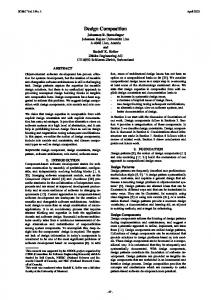
design pattern. The following defines the notion of conformance of a concrete design to a pattern. Definition 2 (Conformance of a design to a pattern) Let m be a model and P =< V, P rs , P rd > be a formal specification of a design pattern. The model m conforms to the design pattern as specified by P if and only if m |= Spec(P ). � Figure 1. Adapter pattern class diagram specification is a ground predicate in the following form. ∃v1 : T1 ∃v2 : T2 · · · ∃vn : Tn .(P rs ∧ P rd )
(1)
In the sequel, we write Spec(P ) to denote the predicate (1) above, V ars(P ) for the set of variables declared in V , and P red(P ) for the predicate P rs ∧ P rd , P reds (P ) for P rs and P redd (P ) for P rd . For example, the following is the specification of the Adapter design pattern. Here, we omit the text descriptions, context and solutions to save space, but we include the diagrams shown in Figure 1 from the GoF book for the sake of readability. Specification 1 (Object Adapter Pattern) Components • T arget, Adapter, Adaptee ∈ classes, • requests ∈ T arget.opers, • specreqs ∈ Adaptee.opers Static Conditions • Adapter −−� T arget, Adapter −→ Adaptee, • CDR(T arget) Dynamic Conditions • ∀o ∈ requests · ∃o� ∈ specreqs · (calls(o, o� )) In Specification 1, CDR(C) stands for client depends on root, where C is the root class. It means that if a message is sent from a class that is not explicitly mentioned in the pattern then the operation must be declared in the root class. Formally, CDR(C) ≡ ∀m ∈ msgs · (toClass(m) ∈ subs(C) ⇒ m.sig ∈ toClass(m).opers ∧ ∃o ∈ C.opers · (toClass(m).o = m.sig)) The specification given above is for Object Adapter. The Class Adapter pattern has the static condition Adapter − −� Adaptee instead of Adapter −→ Adaptee. Moreover, it is only the Adapter class that can send a message to the Adaptee. Formally, ∀m ∈ msgs · (toClass(m) = Adaptee ⇒ f romClass(m) = Adapter)
2.4
Reasoning about patterns
In the practical application of design patterns, it is desirable to prove that a concrete design really conforms to a
The conformance of a model m to a pattern can be easily proved by finding an assignment α of variables in V to elements in m and evaluating P red(P ) in the context of the assignment α. If the evaluation results in true, then the model satisfies the specification. An example of such proofs can be found in [3]. The following theorem proves that such a proof of a model’s conformance to a design pattern is valid. The proofs of the theorems given in this section are omitted, but can be found in [3]. Theorem 1 (Validity of conformance proofs) Let m be a model and P = �V, P rs , P rd � be a specification of a design pattern. The model m conforms to the design pattern as specified by P if and only if there is an assignment α from V ars(P ) to the elements in m such that . Evaα (m, P red(P )) = true. � Given a formal specification of a pattern, we can infer the properties of the systems that conform to the pattern in first order logic. The following theorem proves that properties deduced from the specification in the first order logic are satisfied by all models of the pattern. Theorem 2 (Validity of property proofs) Let P be a formal specification of a design pattern. Spec(P ) ⇒ q implies that for all models m such that m |= P we have that m |= q. � There are a number of different kinds of relationships between patterns. Many of the relationships can be defined as logic relations and proved in first order logic. Specialisation is such a relationship. Definition 3 (Specialisation relation) Let P and Q between design patterns. Pattern P is a specialisation of Q, written P ⇒ Q, if for all models m, it is the case that m conforms to P implies that m also conforms to Q. � The specialisation relation between two patterns can be proved by inference in the first order logic that Spec(P ) ⇒ Spec(Q). The following theorem states that such proofs are valid. Theorem 3 (Validity of proofs of specialisation relation) Let P and Q be two design patterns. Spec(P ) ⇒ Spec(Q) implies that P ⇒ Q, i.e. P is a specialisation of Q. �
3 Composition of design patterns In this section, we will first define some operations on design patterns, then use these operations to formally define the compositions of design patterns.
3.1
Motivating examples
Before we give the formal definition of composition, let’s first see a motivating example. Specification 2 (Composite Pattern) Components • Component, Composite ∈ classes, • Leaf s ⊆ classes, • ops ⊆ Component.opers Static Conditions • CDR(Component), allAbstract(ops) • ∀l ∈ Leaf s · (l −−� Component ∧ ¬(l −→ Component)) • isInterf ace(Component), • Composite −−� Component • Composite −→∗ Component Dynamic Conditions • ∃m ∈ messages · (toClass(m) = Composite ∧ m.sig ∈ ops ⇒ ∃m� ∈ messages · calls(m, m� ) ∧ m� .sig = m.sig) • ∃m ∈ messages · (toClass(m) ∈ Leaf s ∧ m.sig ∈ ops ⇒ ¬∃m� ∈ messages·calls(m, m�)∧m� .sig = m.sig) Consider the Composite and Adapter patterns formally specified in Spec. 2 and 1. Suppose that in the design of a system, we have one leaf class in the Composite pattern and that this class is to be adapted using an Adapter pattern. This specific use of two patterns is a composition of patterns Composite and Adapter. To enable this composition to be specified formally, first we need to specialize Composite pattern so that it only contains one leaf component called Leaf rather than in the general case where there is a nonempty set Leaf s of leaves. Let this specialised Composite pattern be called Composite1 . Moreover, we also need to specify that the component leaf in Composite1 is the adapted component in the Adapter pattern, i.e. the component Leaf in Composite pattern is also the T arget component in Adapter. Finally, to make the result of composition generally useful, we will also rename the components so that their roles can be understood from their names. For example, we would like to name the component Leaf in Composite1 , which overlaps with the T arget in Adapter, to be the AdaptedLeaf . From the above analysis we can see that we need the following operators on design patterns: (a) specialisation of a pattern; (b) composition of pattern with an overlap; (c) renaming the components in a pattern.
Before we formally define the operations and study their properties, let’s see a slightly more complicated composition of design patterns. Specification 3 (Composite1 Pattern) Components • Component, Composite, Leaf ∈ classes, • ops ⊆ Component.opers Static Conditions • CDR(Component), allAbstract(ops) • Leaf −−� Component, ¬(Leaf −→ Component)) • isInterf ace(Component), • Composite −−� Component • Composite −→∗ Component Dynamic Conditions • ∃m ∈ messages · (toClass(m) = Composite ∧ m.sig ∈ ops ⇒ ∃m� ∈ messages · calls(m, m� ) ∧ m� .sig = m.sig) • ∃m ∈ messages · (toClass(m) = Leaf ∧ m.sig ∈ ops ⇒ ¬∃m� ∈ messages·calls(m, m�)∧m� .sig = m.sig) When we compose Composite with Adapter pattern, we may want to adapt a number of leaf components in the Composite patterns. Each of the adapted leaves may have a different adapter. We can apply the above operations to define that there are two adapted leaves, three adapted leaves, etc. However, we cannot define a single pattern that can be applied to all these situations. To achieve this objective, we need an operation on patterns such that the result of an application of lifting on a pattern P is a pattern P � with the following property: that a design model m conforms to P � if it contains at least one set of components that matches pattern P . This operation is called Lif t in the sequel.
3.2
Specialisation
Let’s start with the specialisation operation on patterns. Definition 4 (Specialisation operation) Let P be given pattern and c be a predicate defined on the components of P , a specialisation of P . A specialisation by imposing a constraint c, written as P [c], is the pattern obtained from P by imposing the predicate c as an additional condition of the pattern. Formally, V ars(P [c]) = V ars(P ), P red(P [c]) = (P red(P ) ∧ c) � The following theorem states that by applying a specialisation operation [c] on a pattern P , the result is a pattern that is indeed a specialisation of P . Theorem 4 (Specialisation by constraints) For all patterns P and valid predicates c, P [c] ⇒ P . Proof. By Definition 4, we have that Spec(P [c]) ≡ (Spec(P ) ∧ c) ⇒ Spec(P ). By Theorem 3, we have that Spec(P [c]) ⇒ P . �
Example 1 The pattern Composite1 can be formally defined as follows. Composite1 = Composite[Leaf s = {Leaf }]. By inference in the first order logic, we can simplify Composite1 to the specification in Spec. 3. �
3.3
Proof. (⇒) Let m |= P . By definition 2, there is an assignment α such that Evaα (P red(P ), m) = true. Let α(vi ) = ai . We have that p(a1 , a2 , · · · , an ) is true in model m. Define α� (vsi ) = {ai }, for i = 1, 2, · · · , n. We have that, vsi �= ∅ for all i = 1, 2, · · · k. It is also easy to see that the following predicate is also true under assignment α� . ∀v1 ∈ vs1 · ∀v2 ∈ vs2 · ∀vk ∈ vsk ·
Lifting
Informally, the application of the lifting operation on a pattern P results in a pattern P � such that a design model m conforms to P � if it contains at least one set of components that matches pattern P . We will write P ↑ to denote the result of a lifting on P . So P ↑ is the pattern in whicha model contains a variable number of instances of pattern P . For example, Adapter ↑ is the pattern that the design contains a number of T argets of adapted classes. For each of them, the system has an Adapter class and an Adaptee class configured as in the Adapter pattern. To indicate that the classes Adaptees and Adapters are varying according to the component T argets, we write Adapter ↑ T arget. In other words, the component T arget in the lifted pattern plays a role similar to the primary key in a relational database. Formally, we define the lift operation as follows. Definition 5 (Lift Operation) Let P be a pattern and V ars(P ) = {v1 : T1 , v2 : T2 , · · · , vn : Tn }, n > 0 and Spec(P ) = p(v1 , v2 , · · · , vn ). Let V = {v1 , v2 , · · · , vk }, 1 ≤ k < n, be a subset of the variables of the pattern. The lift of P with V as the key, written P ↑ V , is the pattern defined as follows. V ars(P ↑ V ) = {vs1 : ℘T1 , vs2 : ℘T2 , · · · , vsn : ℘Tn } P red(P ↑ V ) = ∀v1 ∈ vs1 · ∀v2 ∈ vs2 · ∀vk ∈ vsk · ∃vk+1 ∈ vsk+1 · ∃vn ∈ vsn · p(v1 , v2 , ·, vn ) ∧ (vs1 �= ∅) ∧ · · · ∧ (vsk �= ∅) � Example 2 For example, Adapter ↑ {T arget} is the pattern as follows. V ars(Adapter ↑ {T arget}) = {T argets, Adapters, Adaptees ⊆ classes} P red(Adapter ↑ {T arget}) = ∀T arget ∈ T argets · ∃Adapter ∈ Adapter · ∃Adaptee ∈ Adaptees · Spec(Adapter). � Theorem 5 (Lifting Operation) For all patterns P and models m, we have m |= P if and only if m |= (P ↑ V ), where V is any non-empty subset of V ars(P ).
∃vk+1 ∈ vsk+1 · ∃vn ∈ vsn · p(v1 , v2 , ·, vn ) Therefore, we have that m |= P ↑ V . (⇐) Let m |= P ↑ V . By definition 2, there is an assignment α such that Evaα (P red(P ↑ V ), m) = true. Let α(vsi ) = Ai . We have that for all a1 ∈ A1 , · · ·, ak ∈ Ak the following predicate is true in model m. ∃vk+1 · ∃vn · p(a1 , · · · , ak , vk+1 , · · · , vn ) Let ak+1 , · · · , an be the witness of vk+1 , · · · , vn in the above. Then, we have that p(a1 , a2 , · · · , an ) is true in model m. Define assignment α� (vi ) = ai , i = 1, 2, · · · , n. We have that Evaα� (p(v1 , v2 , · · · , vn ), m) = true. That is, m |= P . �
3.4
Overlaps
Consider a situation in which a design model m conforms to two design patterns P and Q at the same time. Thus, by the definition of conformance and Theorem 1, we have that there is an assignment α1 such that Evaα1 (P red(P ), m)= true, and at the same time there is an assignment α2 such that Evaα2 (P red(Q), m)= true. An overlap between two assignments in the conformances means that there is at least one element in model m involved in both assignments α1 and α2 . Such an involvement can be in one of the following three cases. Case 1: One to one overlap. In this situation, there is one element in the model m assigned to a variable of pattern P by α1 and at the same time the same element is also assigned to a variable in pattern Q by α2 . This element in the design model m plays two roles; one for each of the design patterns. In this case, we say the overlap is an oneto-one overlap. Let v ∈ V ars(P ) and v � ∈ V ars(Q) be the variables that are assigned to the same element in model m. Therefore, the model m does not only conform to P and Q (thus satisfy the condition P red(P )∧P red(Q)), but also satisfies the condition that v = v � . We will also name the new role that the overlap element plays in the composition, say v �� . Therefore, we also have the equations that v �� = v and v �� = v � for the composition pattern. These equations are called the overlap constraints. Case 2: One to many overlap. In this situation, there is an element in the model m assigned to a variable of pattern P by α1 , and at the same time there is a set E of elements such that E is assigned to a variable v � in pattern Q. In this case, we say the overlap is an one-to-many overlap. Assume
that the variable v is of type T , e.g. the type Class. Then, the variable v � must be of type P T , e.g. a subset of classes. Because variables v and v � are of different types, we cannot simply write the overlap constraints as equations. Instead, we will lift the pattern P , thus variable v becomes variable vs, which is of type P T . Assume that the new role that the overlap part plays is called v �� . The overlap constraints are v �� = vs and v �� ⊆ v � . Case 3: Many to many overlap. In this case, there is an element in the model m in a set E of elements assigned to variable v in pattern P by α1 , and at the same time it is in another set E � of elements that are assigned to variable v � in pattern Q by α2 . In this case, both variables must be of the same type of PT . In this case, we say the overlap is a many-to-many overlap. Assume that the new role of the overlap part played in the composition pattern is called v �� . Then, the overlap constraints are v �� ⊆ v and v �� ⊆ v � . The following definition introduces a notation to represent various types of overlaps [3]. For the sake of simplicity, we assume that V ars(P ) ∩ V ars(Q) = ∅. This can always be achieved by systematically renaming the variables in V ars(P ) and their free occurrences in P red(P ). Definition 6 (Overlaps) Let P and Q be two patterns. We write vnew := (v : P #v � : Q) to denote an overlap between the component v in pattern P with component v � in pattern Q, and the overlapped part is named as vnew , where vnew �= V ars(P ) ∪ V ars(Q). When there is no risk of confusion, we will omit the names of patterns and write simply vnew := (v#v � ). An overlap vnew := (v#v � ) is called an one-to-one overlap and written vnew := v −−v � , if both v and v � are of type T . It is called a many-to-many overlap and written vnew := v >−< v � , if both v and v � are of type PT . In both one-to-one and many-to-many overlaps, we say that the variables v and v � are equally ordered. The overlap is called a many-to-one overlap and written vnew := v >−− v � or vnew := v −−< v � , if v is of type PT and v � is of type T , or vice versa. In this case, we say that v is higher ordered in the overlap and v � lower ordered. Let o be a set of overlaps as defined above between pattern P and Q. We write V arsP (o) to denote the subset of variables in V ars(P ) that occurred in o. We say that P is lower ordered, if there is a variable in V arsP (o) that is lower ordered. �
P red(P ⊗o Q) = P red(P � ) ∧ P red(Q� ) ∧ OC(o). Here U � = U ↑ V arsU (o) if U is lower ordered in o; otherwise U � = U , U = P, Q. N ewV ars(o) is the set of new variables given in overlap o. Predicate OC(o) is the conjunction of overlap constraints. Formally, let o = {u1 := v1 #v1� , · · ·, un := vn #vn� }. OC(o) = OC(u1 := v1 #v1� ) ∧ · · · ∧ OC(un := vn #vn� ) OC(u := v#v � ) ⎧ (u = v ∧ u = v � ), ⎪ ⎪ ⎨ (u ⊆ v ∧ u ⊆ v � ∧ u �= ∅), = ⎪ (u ⊆ v ∧ u = vs� ∧ u �= ∅), ⎪ ⎩ (u = vs ∧ u ⊆ v � ∧ u �= ∅), �
In the above definition, variables vs and vs� are the corresponding lifted variables of v and v � , respectively. Example 3 Now, we return to the motivating example of the composition of Composite1 and Adapter with the overlap that the Leaf component in Composite1 is the same as component T arget in the Adapter pattern. We name this overlapped component AdaptedLeaf in the result pattern of the composition. This overlap can be specified as AdaptedLeaf := Leaf #T arget. It is an one-toone overlap. Let o1 be this overlap. Thus, the composition with o1 is the pattern Comp1 Adapter = Composite1 ⊗o1 Adapter. By Definition 7, we have that V ars(Comp1 Adapter) = {Composite, Component, Leaf, Adapter, Adaptee, T arget, AdaptedLeaf } P red(Comp1 Adapter) = P red(Composite) ∧ P red(Adapter) ∧
�
(AdaptedLeaf = T arget) ∧ (AdaptedLeaf = Leaf )
Example 4 For the composition of Adapter with Composite (rather than Composite1 ), the overlap o2 is T Leaf s := Leaf s#T arget. This is a one-to-many overlap with T arget as the lower ordered variable. Let CompAdapter = Composite ⊗o2 Adapter. By Definition 7, we have that V ars(CompAdapter) = {Composite, Component ∈ classes, Leaf s, T Leaf s, Adapters, Adaptees, T argets ⊆ classes} P red(CompAdapter) =
We can now define composition with an overlap. Definition 7 (Composition with an overlap) Let o be a set of overlaps between pattern P and Q. The composition of P and Q with overlap o, written P ⊗o Q, is a pattern defined as follows.
(T Leaf s ⊆ Leaf s) ∧ (T Leaf s = Adapters) ∧ P red(Composite) ∧ (T Leaf s �= ∅) ∧ ∀Adapter ∈ Adapters · ∃T arget ∈ T argets ·
V ars(P ⊗o Q) = V ars(P � ) ∪ V ars(Q� ) ∪ N ewV ars(o),
u := v −−v � ; u := v >−< v � ; u := v >−− v � ; u := v −−< v � ;
�
∃Adaptee ∈ Adaptees · P red(Adapter)
As one would expect, we have the following theorem about composition as defined above.
This lifts the variables Context and Strategy to sets and introduces a new component ContextLeaf s. This yields the following pattern.
Theorem 6 (Composition of Patterns) Let P and Q be any given patterns and o any overlap between P and Q. For all models m, m |= P ⊗o Q implies that m |= P and m |= Q.
V ars(Composite ⊗o3 Strategy) =
Proof. Let o be any given overlap between patterns P and Q. If P is lower ordered, by Definition 7, we have that P red(P ⊗o Q) ⇒ P red(P ↑ V arsP (o)). Therefore, by Theorem 3, we have that for all models m, m |= P red(P ⊗o Q) implies that m |= P red(P ↑ V arsP (o)). By Theorem 5, we have that for all models m, m |= P red(P ↑ V arsP (o)) if and only if m |= P red(P ). Thus, we have that for all models m, m |= P red(P ⊗o Q) implies that m |= P red(P ). Similarly, when P is not lower ordered, by Definition 7, we have that P red(P ⊗o Q) ⇒ P red(P ). By Theorem 3, we have that m |= P red(P ⊗o Q) implies that m |= P red(P ). Therefore, in all cases, we have that for all models m, m |= P ⊗o Q implies that m |= P . The same proof applies to Q. Therefore the theorem is true. �
⊆ classes} P red(Composite ⊗o3 Strategy) =
4 Example and case study This section illustrates how the notion of composition with overlaps can be apply to define compositions of design patterns and reports a case study on the expressiveness of the composition operators defined in this paper.
4.1
Example: The MVC Pattern
As a more complicated example of pattern composition, we now show that the M V C pattern can be formed by composing Composite, Strategy and Observer patterns. The specifications of Strategy and Observer are given below. Specification 4 (Strategy Pattern) Components: • Context, Strategy ∈ classes, • conInt ∈ Context.opers, • algInt ∈ Strategy.opers Static Conditions • Context −→ Strategy, isAbstract(algInt) Dynamic Conditions • callsHook(conInt, algInt) We first compose Composite to Strategy with a manyto-one overlap o3 . o3 = {ContextLeaf s := Leaf s >−− Context, OpContext := operation −−conInt)}.
{Composite, Component ∈ classes, Leaf s, Contexts, Strategies, ContextLeaf s
P red(Composite) ∧ P red(Strategy ↑ {Context}) ∧ (ContextLeaf s ⊆ Contexts) ∧ (ContextLeaf s �= ∅) ∧ (ContextLeaf s ⊆ Leaf s) However, because of the lifting of the variable Strategy to Strategies, the composition pattern has several Strategy classes, each the root of a separate hierarchy. This seems strange. In the Java API, the single class ActionListener is used. So we shall assume for simplicity that every class in the set Strategies is equal to a variable Strategy. This can be formally expressed as a constraint on the composition of the patterns by a predicate Strategies = {Strategy}, thus we have Composite ⊗o3 Strategy[Strategies = {Strategy}] It is easy to prove that it is equivalent to the following pattern P V C by inference in the first order logic. V ars(P V C) = {Leaf s ⊆ classes, Composite, Component, Context, Strategy ∈ classes} P red(P V C) = (Strategy ∈ Leaf s)∧ P red(Composite) ∧ P red(Strategy) Specification 5 (Observer Pattern) Components: • Subject, Observer ∈ classes, • update ∈ opers(Observer) Static Conditions • Subject −→∗ Observer, ¬update.isLeaf , • ∀O ∈ subs(Observer). (∃S ∈ subs(Subject) . O −→ S) Dynamic Conditions • ∃ms ∈ messages . ¬ms.sig.isQuery∧ toClass(ms) ∈ subs(Subject) ⇒ • ∃m ∈ messages · m.sig = notif y∧ f romLL(m) = toLL(m) = toLL(ms)∧ • ∃mu, mg . mu.sig = update ∧ isQuery(mg.sig) ∧toLL(mu) = l ∧ calls(m, mu)∧ calls(mu, mg) ∧ toLL(mg) = toLL(ms) Then, we further compose this to Observer with the following overlap o4 .
o4 = {StrObs := Strategy −−Observer} Let M V C = P V C ⊗o4 Observer. By definition, we have that V ars(M V C) = {Composite, Component, Subject, Observer, StrObs ∈ classes, Leaf s, Contexts, Strategy, ContextLeaf s ⊆ classes} P red(M V C) = P red(Observer)∧ P red(Composite) ∧ P red(Strategy) ∧ (Strategy ∈ Leaf s) ∧ StrObs = Strategy ∧ StrObs = Observer This is exactly the M V C design pattern.
4.2
Case Study of GoF patterns
In [9], possible compositions of patterns were suggested in the Related Patterns section of each pattern. Such discussions were informal and little details were given. However, having formally defined the notion of compositions of patterns, we can now formalise all of these suggestions using the notion of overlap. For example, it is stated that an Abstract Factory can create and configure a particular Bridge [9] (p161). This suggests that the Abstract and Implementor components in the Bridge pattern are the AbstractP roducts in the AbstractF actory pattern. Thus, the overlap is o = {AbstractP roduct >−− Abstraction, AbstractP roduct >−− Implementor} By composing AbstractF actory pattern and Bridge pattern with the overlap o, we can see that the Client’s dependences on Abstract and Implementor components in the Bridge pattern can be satisfied because of the constraints on AbstractP roduct in the AbstractF actory pattern. All other conditions relate AbstractP roducts to the other classes in the AbstractF actory pattern and so are not relevant. It is also suggested that Iterator can be used to implement the recursion in Composite pattern [9]. The overlap is between the ConcreteAggregates in Aggregate pattern and the Component in Composite pattern. In our formal specification given in [4], ConcreteAggregate was implicitly referred to as subs(Aggregate). To enable composition with overlaps be defined, we first apply the specialisation operation to Iterator, i.e. define Iterator� as follows. Iterator[ConcreteAggregates = subs(Aggregate)] Then, we compose Iterator� to Composite with the overlap ConcreteAggregates >−− Component. Table 2 summarises the overlaps between GoF patterns, where Command� is defined in a similar way to Iterator� .
Details of these compositions and the proofs of their satisfiability are omitted for the sake of space and will be reported separately. Our case study demonstrated that our operations on design patterns and our compositions of design patterns are expressive and general enough to cover the suggested compositions made in GoF book [9]. Table 2. Summary of Case Study Patterns Overlap Abstract Factory {AbsProducts >− −Abstr, + Bridge AbsProducts >− −Implem} Composite + Decorator {Component − − Component, Composite − − Decorator, operation − − operation} Component + Flyweight {Component − − Flyweight} Iterator’ + Composite {ConcreteAggregates >− −Component} Visitor + Composite {Component − − Element} Abstract Factory {AbstractFactory + Facade − − Facade} Facade + Singleton {Facade − − Singleton} State + Flyweight {State − − Flyweight} Strategy + Flyweight {Strategy − − Flyweight} Chain of Resp {Chain of Resp + Composite − − Composite} Command + Composite {Command − − Component} Memento + Command’ {Caretaker − − ConcreteCommands} Prototype + Command {Prototype − − Command} Iterator {Iterator − − Product} + Factory Method Iterator’ + Memento {ConcreteIterators >− − Caretaker} Mediator + Observer {Colleague − − Observer, Mediator − − Subject} State + Singleton {State − − Singleton} State + Flyweight {State − − Flyweight} Strategy + Flyweight {Strategy − − Flyweight}
5 Conclusion In this paper, we further developed our method for the formal specification of design patterns by adding a formal definition of the composition of design patterns. The properties of compositions are proved. A case study of the relationships between design patterns as suggested by GoF [9] is reported. As demonstrated in this paper, formal reasoning about design patterns and their compositions can be naturally supported by the formal deduction in first order logic, which is well understood, and well supported by software tools such as theorem provers. There are a large number of papers published in the literature on formalisation of software design patterns. Existing
work can be classified into two categories. The first category proposes special-purpose formal languages or semiformal graphic modeling languages in order to define patterns rigorously [14, 6, 7]. The second category, to which our work belongs, simply employs or adapts existing formal or semi-formal languages [12, 18, 19, 15, 10, 13, 8, 20]. While each of these approaches are demonstrated with examples, it remains an open question whether they can be used to specify all design patterns. Our approach has been proven to be expressive by the successful specification of all 23 design patterns in the GoF catalog [2, 5]. In the existing work, few have attempted to facilitate formal reasoning about design patterns even though formalisation is perceived to have the potential to support formal reasoning. Generally speaking, for the works in the first category summarized above, to support formal reasoning of design patterns, a formal logic must be devised and its logic properties, such as semantic consistency must be proven and a special purpose formal reasoning tool must be developed. Thus, a great effort must be made before they can become practically useful. For works in the second category, those using the UML meta-modeling facility suffer from the ambiguity and informal definition of UML. Even the basic notion that a concrete design conforms to a pattern has to be defined with great length [8]. Few works on formal definition of pattern composition has been reported in the literature. One such work is by Taibi [18]. He discussed the composition of design patterns specified in the balanced pattern specification language BPSL. His definition did not handle the most complicated form of pattern composition like the many-to-many kind of overlaps, however. In comparison with existing works, the formal specifications of design patterns in our approach are natural and easier to understand. Our approach is highly expressive. As demonstrated in this paper, reasoning about design patterns on various kinds of properties and relationship as well as their compositions can be naturally supported by the wellunderstood first order logic. Such reasoning can also be supported by software tools such as first order logic theorem provers. We are investigating the uses of theorem provers for automated reasoning about design patterns based on the theory developed in this paper.
References [1] D. Alur, J. Crupi, and D. Malks. Core J2EE Patterns: Best Practices and Design Strategies. Prentice Hall, 2nd edition, June 2003. [2] I. Bayley and H. Zhu. Formalising design patterns in predicate logic. In 5th IEEE International Conference on Software Engineering and Formal Methods, 2007. [3] I. Bayley and H. Zhu. Formal reasoning about design patterns. In 10th International Conference on Formal Engineering Methods (ICFEM 2008) (Submitted to), 2008.
[4] I. Bayley and H. Zhu. Specifying behavioural features of design patterns. Technical Report TR-08-01, Department of Computing, Oxford Brookes University, Oxford, UK, 2008. [5] I. Bayley and H. Zhu. Specifying behavioural features of design patterns in first order logic. In 32nd IEEE International Conference on Computer Software and Applications (COMPSAC 2008), 2008. [6] A. H. Eden. Formal specification of object-oriented design. In International Conference on Multidisciplinary Design in Engineering, Montreal, Canada, November 2001. [7] A. H. Eden. A theory of object-oriented design. Information Systems Frontiers, 4(4):379–391, 2002. [8] R. B. France, D.-K. Kim, S. Ghosh, and E. Song. A umlbased pattern specification technique. IEEE Trans. Softw. Eng., 30(3):193–206, 2004. [9] E. Gamma, R. Helm, R. Johnson, and J. Vlissides. Design Patterns - Elements of Reusable Object-Oriented Software. Addison-Wesley, 1995. [10] A. L. Guennec, G. Suny´e, and J.-M. J´ez´equel. Precise modeling of design patterns. In UML 2000 - The Unified Modeling Language. Advancing the Standard. Third International Conference, York, UK, October 2000, Proceedings, volume 1939, pages 482–496. Springer, 2000. [11] D. Hou and H. J. Hoover. Using SCL to specify and check design intent in source code. IEEE Transactions on Software Engineering, 32(6):404–423, June 2006. [12] K. Lano, J. C. Bicarregui, and S. Goldsack. Formalising design patterns. In BCS-FACS Northern Formal Methods Workshop, Ilkley, UK, September 1996. [13] J. K. H. Mak, C. S. T. Choy, and D. P. K. Lun. Precise modeling of design patterns in uml. In 26th International Conference on Software Engineering (ICSE’04), pages 252– 261, 2004. [14] D. Mapelsden, J. Hosking, and J. Grundy. Design pattern modelling and instantiation using dpml. In CRPIT ’02: Proceedings of the Fortieth International Conference on Tools Pacific, pages 3–11. Australian Computer Society, Inc., 2002. [15] T. Mikkonen. Formalizing design patterns. In Proc. of ICSE’98, Kyoto, Japan, pages 115–124. IEEE CS, April 1998. [16] N. Nija Shi and R. Olsson. Reverse engineering of design patterns from java source code. In Proc. of ASE’06, Tokyo, Japan, pages 123–134, September 2006. [17] OMG. Unified modeling language: Superstructure, version 2.0, formal/05-07-04. [18] T. Taibi. Formalising design patterns composition. Software, IEE Proceedings, 153(3):126–153, June 2006. [19] T. Taibi, D. Check, and L. Ngo. Formal specification of design patterns-a balanced approach. Journal of Object Technology, 2(4), July-August 2003. [20] U. Zdun and P. Avgeriou. Modelling architectural patterns using architectural primitives. In 20th annual ACM SIGPLAN conference on Object-Oriented Programming, Systems, Languages and Applications (OOPLSA), San Diego, California, pages 133–146, 2005. [21] H. Zhu and L. Shan. Well-formedness, consistency and completeness of graphic models. In Proc. of UKSIM’06, Oxford, UK, pages 47–53, April 2006.