Given a path profile, and a maxin~um avalanche speed, then it is possible ...... 6.5. Granite Creek 7. 1080. 66.6. 66.5. 65.9. 56.5. 23.5. 7.4. Granite Creek 9. 1049.
On the computation of parameters that model snow avalanche motion S. BAKKEH@I
Can. Geotech. J. Downloaded from www.nrcresearchpress.com by Renmin University of China on 05/28/13 For personal use only.
Norwegiar~Geotechtlical Itzstitrtte, Box 40, Tdset~,Oslo, Norway Water Survey of Canada, Etzvirotlmetlt Car~ada,Calgary; Alto., Catluda
U. DOMAAS AND K. LIED Norrsegiatz Geotechr~icnlIrlstitrtte, Box 40, Tdserl, Oslo, Norway
Nariotlnl Hydrology Resecrrcll Itlstiture, Ei~vironnlerltCanada, Ottnlva, Ont., Carlada AND
Itld~rstriellHydro-og Aerodyr~at?zikk,Bogsrav 11, Oslo, Norway Received May 14, 1980 Accepted October 7, 1980 This paper explores the computational problem of finding suitable numbers to use in a twoparameter model of snow avalanche dynamics. The two parameters are friction, y, and a ratio of avalanche mass t o drag, MID. Given a path profile, and a maxin~umavalanche speed, then it is possible to compute unique values for p and MID. If only the path profile and the stopping position are known, then it is possible t,o compute tables of pairs (p,M I D ) which can be tested as predictors of avalanche speeds. T o generate these tables it is convenient to scale M I D in multiples of the total vertical drop of the path. The computations were tested on 136 avalanche paths. Values of (p,M I D I were stratified, and certain values were rejected as unrealistic. Le problkme analytique de la dCfinition des nombres B utiliser dans un modkle deux parametres de la dynamique des avalanches de nei e est CtudiC dans cet article. Les deux paramktres sont le frottement p et le rapport de la masse $e l'avalanche B la risistance MID. Pour un profil de trajectoire et une vitesse d'avalanche maximum donnCs, il est possible de calculer des valeurs uniques de p et MID. Si on connait seulement le profil de trajectoire et la position dYarrCt,il est alors possible de calculer des tables de couples {p, M / D ] qui peuvent Ctre utilisCs pour la prediction des vitesses d'avalanches. Pour dCvelopper ces tables, il est pratique d'exprimer MID en multiples de la denivelie totale de la trajectoire. Les calculs ont CtC vCrifiCs sur 136 trajectoires d'avalanches. Les valeurs de (p, M I D 1 ont CtC stratifiees et certaines valeurs ont CtC rejetCes comme irrealistes. [Traduit par la revue] Can. Geotech. J., 18, 121-130 (1981)
Introduction A consultant who specializes in snow avalanche behaviour often faces the dilemma of preparing a map which shows the extreme runout boundaries of an avalanche. In some cases, the specialist will also need to estimate the avalanche speeds and impact forces within these boundaries. These questions are preferably answered by studying geomorphological and historical evidence, principally landscape damage, property damage, and personal experiences. If such evidence is unavailable, the runout distance and impact forces may be guesses based on comparison with a similar path where the parameters are known to useful precision. Such comparison is necessarily biased by subjective interpretation. This is not always
satisfactory where land values are high, and subjective decisions are strongly questioned. There are also computations that can be used in place of, or along with, the subjective estimates. For example, Voellrny (1955) developed equations for the avalanche speed and runout distance that were analogous to equations used in the theory of open channel JEolo. Revised versions of his equations are routinely applied, although not without reservations because his main parameters are often chosen subjectively. The purpose of this paper is to study the numerical computation of two parameters that are crucial to the determination of avalanche speed and runout distance. To develop our avalanche model, we begin
0008-3674/81/010121-10$01.00/0
@ 1981 National Research Council of Canada/Conseil national de recherches du Canada
Can. Geotech. J. Downloaded from www.nrcresearchpress.com by Renmin University of China on 05/28/13 For personal use only.
122
CAN. GEOTECH. J. VOL. 18, 1981
with what seem to be arbitrary assumptions, but we will end up with two parameters that are analogous to those which appear in Voellmy's equations. Thereafter, our numerical system for determining the values of these parameters on the basis of field observations is fully applicable to Voellmy's model as well as our own. Although our examples are limited to snow avalanches, our methods may have wider application to other types of mass movement.
Profile Model An example of an avalanche map and path profile is shown in Fig. 1. In Inany cases, the avalanche path does not deflect sharply to the side, and it seems reasonable to transcribe the centre line of the path onto a flat, vertical surface, duplicating the total length of the centre line from the top to the bottom boundaries of the avalanche path, and duplicating all vertical distances. We will analyse profiles that are prepared in that fashion, although the equations and solutions we present are easily generalized to treat a centre line that deflects to the side. Many avalanche profiles are broken up by cliff bands, thus the mathe-
matical approximation for the profile may be a rather complicated, perhaps multivalued function containing one or more inflections. We assume the ii7ciss ce11tr.eof the avalanche moves with tangential speed o(s), where s is the distance measured from the top of the path. For reasons we now discuss, we are forced to assume that the initial rest position, u = 0, is at the top point of the profile, and that the final stop position is at the bottom point, that is, the extreme lower boundary of the profile. In reality, the mass centre does not move between the observed limits of the path, but depending on the spatial extension of the moving mass probably begins -- 10 to -- 100 m below the observed top boundary, and comes to rest -- 10 to -- 100 m above the bottom boundary. The end result of assuming that the n~asscentre moves between the extreme limits is to shift the values of the two empirical parameters that we shall introduce in the next section. However, if we are consistent in our method of assigning path length, and if we exclude from our analysis snlall avalanche paths where the path length is comparable to the dimensions of the moving mass, then this shift should not seriously alter our results. Unfortunately, the effects
2 ILOO J
1
0
I
200
I
LOO
I
600
I
I
I
800 1000 1200 DISTANCE ( m )
I
ILOO
I
1600
I
1800
I
2000
FIG. 1. Map and profile of the Ryggfonn avalanche path (near Stryn, Western Norway). Top and bottom dots on profile denote boundaries of largest (extreme) known event. Intermediate dots represent end points of segments for approximating profile (as explained later in text).
123
Can. Geotech. J. Downloaded from www.nrcresearchpress.com by Renmin University of China on 05/28/13 For personal use only.
B A K I C E H ~ IET AL.
of the shift are difficult to test since the actual rest positions of the mass centre are generally unknown for the extreme events. For the cases under consideration the total path length is -- 1000 m compared with our estimate (no firm data being available) that the spatial extent of over half the moving mass during the extreme event was confined to 100 m. Another complicating factor is entrainment. As an avalanche descends, snow is deposited continuously onto the path, and at the same time new snow is entrained into the moving mass, which may be increasing or decreasing at any time (or position s). We will not require that the mass remain constant, as is often done in dynamic avalanche computations, but we will adopt the simplest assumptions, i.e., that for any position, s, all mass is entrained from rest to u(s), and all mass is dropped out from u(s) to rest. An alternative to the mass-centre model is to emphasize the spatial extension of the mass and to model the avalanche as a fluid in an open channel, focusing attention on the velocity of a column in the fluid. This viewpoint, first studied by Voellmy, offers the possibility of bringing the hydraulic radius of the path into the calculations in order to compute the flow height and mass distribution. However, in its present application (Leaf and Martinelli 1977; Buser and Frutiger 1980) the fluid theory is not used to yreclict flow height in the runout zone, but instead the flow height in the runout zone is guessed, and this guess is used in the calculation of the stopping distance. In essence, Voellmy's calculation of stopping distance reduces to the calculation for a mass centre on a path centre line. In principle, it may be possible to compute flow heights in the runout zone, but in our opinion there are presently too few data to substantiate such calculations. On the other hand, we have considerable data describing runout distances on path profiles, and we have at least some data on avalanche speeds, therefore we can test certain aspects of the masscentre model.
-
of s. After dividing by M, we see that solutions for v on a given profile O(s) depend on two parameters, p. and DIM. The first parameter, p., is dimensionless, and may be interpreted as a friction coefficient in the sense that the avalanche has a weight component (Mg cos 0) perpendicular to the slope. The second parameter which we find more convenient to use in its inverted form, MID, may be interpreted as a ratio of avalanche mass to drag. In the derivation of [I], the inertial effects due to entrainment (dM/ds) and centripetal force (v2/r) due to any curvilinear motion of local radius r are also included in D, which is in kg/m. The parameter M I D therefore is in units of length (m). Since a major portion of this paper is about p. and MID, the notation {p., M I D ) is used for the sake of brevity, thus pairing the nondimensional p with the length MID. In future models a nondimensional parameter replacing M I D may provide additional insight. For example, we could just as well introduce the nondimensional pair {p., M/DL) ,where L is some intrinsic length. Later in this paper we shall return to the question of scaling MID, and propose one possibility for a length scale intrinsic to the avalanche profile. We emphasize that a strict physical interpretation of the pair {p., M I D ] is neither justified nor crucial to our model. We regard { p., M I D ) as an empirical pair chosen to best match (or predict) two observations: the stop position and the maximum speed VM. In our computations {p., M I D ) is held constant for the entire path, whereas in reality resistive and inertial forces probably vary drastically from start to finish. On an infinitely long slope of constant inclination, an avalanche accelerates to the asymptotic solution of [I], [2] S-a lirn v(s)
=
2
1
7
-g (sin 0 - p. cos 0)
Equations [I] and [2] are analogous to Voellmy's equations except that Voellmy uses (p., [h] where [ is a coefficient of dynamic drag, and h is the flow height. Equation of Motion As in our model, Voellmy interprets p. to be a friction coefficient. The conversion between our MID The derivation of our equation of motion is covered in earlier papers (Perla 1980; Perla et 01. 1980). parameter and Voellmy's [h is simply th/g = MID. Briefly, v(s) is approximated by solving the linear Numerical Solution equation At the outset we recognized the need for solving M dv2 [I] -- = Mg(sin O - p. cos 0) - Dv2 [l] numerically on a high speed digital computer. We 2 ds found it impractical to use Korrier's (1980) graphical where M is the avalanche mass, O is the slope angle, solutions since in our study we computed avalanche p. is a coefficient of friction, and D is a coefficient of motion for 136 avalanche paths of varying comdynamic drag. In general, M, 0, p., and D are functions plexity.
Can. Geotech. J. Downloaded from www.nrcresearchpress.com by Renmin University of China on 05/28/13 For personal use only.
124
CAN. GEOTECH. J. VOL. 18, 1981
FIG.2. Segment i and segment i
+ 1.
Our solution is based on approxin~atinga path profile by straight line segments. The segment end points are often determined by natural inflections in the terrain. Typically, about 10 segments adequately approximate a profile. As an example, the profile of Fig. 1 is divided into 9 segments. Our computer model is dimensioned for 100 segments, which is more than adequate considering other contingencies. Figure 2 shows two adjacent segments. Each segment is assigned an angle O i and a length Li. Tn the version of the program described in more detail by Cheng and Perla (1979), the user may either specify pi and (M/D)i for the ith segment, or may input one pair (p., M I D ) for the entire profile. If the speed at the beginning of ith segment is Vi" and the avalanche does not stop somewhere in the middle of the segment, then the speed at the end of the ith segment is the solution to [I],
This introduces a large correction for an abrupt slope change (avalanche dropping over cliff and impacting on benched terrain), but only small corrections where a smooth concave profile is approximated by a large number of straight segments. For a convex configuration, Oi+l > Oi, we do not use [5], but instead set Vi+lA= ViB. Here, we envision that the avalanche is free to follow a more gradual curve around the transition, and that the centripetal lifting force decreases resistive friction, thus compensating somewhat for the momentum loss of the avalanche impacting on the lower segment. Although it has not been a problem in our computations so far, the concave correction [5] could give unrealistic results for extreme cases. As an example, [5] yields ~ i + = ~ " 0 for a cliff band (0i = x/2) above a horizontal bench (Oi = 0). Therefore the segment length must be selected sufficiently large to smooth over cliff bands and benches that are very small compared to the size of the moving avalanche. Despite this difficulty, we feel that it is essential to include some type of correction which differentiates smooth from highly inflected terrain, and [5] is one of the simplest options. Our program allows the user to repeat a profile computation any number of times with new choices of (p., MID 1 . For virtually all practical cases, computation costs are relatively low; central processing time is normally less than 1 s. Sample computations for the profile of Fig. 1 are summarized in Table 1. Outputs I and I1 are based on respective inputs of (0.2, 1000 m ) and 10.1, 500 m ) which were chosen arbitrarily from a group of trial values.
Computation Problems Whether one uses our {p., M I D ) or Voellmy's {p., [ h ) ,there is the same problem of how to choose with ai = g(sin O i - pi cos Oi); pi = -2Li/(M/D)i. values consistent with field observations. As emphaIf the avalanche stops at a mid-segment position, sized by Korner (1980), field observations for the the stopping distance S from the beginning of the ith entire path should be matched as nearly as possible. segment is the solution to [I], If we are given a path profile, a stop position, and a maximum speed, ViLI, we can compute a unique (p., M I D ] . For example, according to measurements made on 25 February 1975, the lead edge of the The solution marches successively downslope from Ryggfonn avalanche (Fig. 1, Table 1) stopped a t the initial rest position. As a first approximation, about 110 m measured up from the Grasdola. SomeVi+l" could be set equal to ViB, but this is improved where at midslope the avalanche developed speeds of by including a correction for the momentum lost at at least 45 m/s (Tgndel 1977; and personal comthe slope transition. In our model we apply a correc- munications). By comparing outputs in Table 1, we tion only if the slope is concave, that is, if 0i > Oi+l, see that (0.1, 500 m ) provides the closer match to these data. By trial and error we can force a more in which case we set exact match. For example, 10.12, 500 m j predicts a V M = 46 m/s and a stop position at 106 m up from [5] Vi+lA = ViB COS (Oi - Oi+,)
1
ViB = l / g i ( g ) i ( l
-
exp pi)
+ (v,")'
exp
pi
BAKKEHQII ET AL.
TABLE 1. Computations for the Ryggfonn avalanche profile (Fig. 1)
Input
Output I1 p = 0.1, MID = 500rn
i
0, ideg)
L, (m)
VA (m/s)
VB (m/s)
(m/s)
1 2 3 4 5 6 7 8 9
37.6 57.5 31.1 20.3 31.1 33.0 25.1 9.0 -9.5
82 65 280 288 397 358 353 192 182
0 26 34 45 43 52 56 50 38
26 38 46 43 52 57 53 40 -
0 27 34 42 37 44 46 40 29
Segment
Can. Geotech. J. Downloaded from www.nrcresearchpress.com by Renmin University of China on 05/28/13 For personal use only.
Output I p = 0.2, MID = 1000 m
Avalanche stops 171 rn on segment i = 9
Grasdola. The trial and error can be made to converge using algorithms of the type discussed later. Comparing outputs I and I1 in Table 1, we note that a -100% variation in {p., MID) results in a -- 10% variation in both Vbr and the stop position (the latter referred to the top reference point). Looked at another way, outputs that are not very different from one another are predicted by markedly different {p., MID).Thus, we expect difficulty narrowing the choice of {p., MID)since avalanche field observations usually consist of many uncertainties. The verification problem intrinsic to our model (and to Voellmy's as well) is largely traceable to the competing influence of y and MID in the equation of motion (our [I]). For the present it is difficult to see how this problem can be avoided in a two-parameter model. There are related problems. Using one pair {y, MID),we are not free to uniquely match three conditions: VRI,stopposition, and position of V M .On the contrary, after selecting {p., MID)to match two conditions, the accuracy with which we predict the third condition furnishes an independent test of the model. The experimental complication is that on highly inflected terrain there may be more than one point where dv/ds = 0, and it could be difficult to establish the position of the absolute maximum speed. Can we determine the variation of {?., MID)with position? No, not even if we were fortunate enough to measure v(s) precisely from start to finish. This can be understood if we picture an avalanche changing speed from V-' to VB over a distance AL. Given VA, there is an unlimited number of {p.,MID)which predict the same VB. The above questions are raised mainly to put our problems in perspective, because it would be indeed
VA
VB (rn/s)
27 38 42 37 44 47 42 30 -
Avalanche stops 122 m on segment i = 9
fortuitous to obtain a detailed measurement of v(s) during an extreme event on a relatively large avalanche path (-1000 m long). Instead, we will use available data describing extreme limits of the profile to establish the reasonable range of {y, MID).This range will then have to be consistent with the few available data describing maximum speeds. Topographical Shape and Scale Factors The range of {p., MID}should first of all be consistent with existing measurements of avalanche topography. Over 400 avalanche paths in Western Norway were mapped and analysed statistically by Lied and Bakkehrai (1980), who proposed that profiles for extreme events could be characterized by a set of topographical values. With reference to Fig. 3a, the variables of interest for our present study are the angles a and @,and the total vertical drop Y. The angle a is determined on a profile by the line connecting the end points for the largest known (extreme) event. The angle @ has a more arbitrary definition. It is determined by the line connecting the top point and a point on the profile where the slope angle is 10". Considered together, a and 8 provide a very simple shape factor. Lied and Bakkehrai had no strong reason to favour a 10" criterion, but nonetheless they showed that a shape factor defined in this way could be used in a regression analysis to determine maximum runout. They went on to develop more rigorous shape factors based on fitting parabolas to the profiles. Using the idea of a simple shape factor based on two angles, we show in Fig. 3b a two-segment approximation in which the shape factor is determined
Can. Geotech. J. Downloaded from www.nrcresearchpress.com by Renmin University of China on 05/28/13 For personal use only.
126
CAN. GEOTECH. J. VOL. 18, 1981
..... . ..
influenced more by variation of shape factor from path to path than by variation in 4 Y. Nevertheless, the influence of 4 Y should not be ignored as was done by Voellmy, and all subsequent users of his theory. In the next section, we will show how Y can be introduced in the more general case, when D is not equal to zero.
Simulation of p, MID, and VM The relationships are greatly complicated when D is not zero, in which case the motion is now determined by the two parameters (y, MID}. Here, there (a) is no simple expression analogous to [6], even for a two-segment approximation. Given only the profile and stop position, we cannot uniquely choose {y, MID]. However, we are able to generate various pairs of {y, MID) which match the stop position. Each pair predicts a different V ~ Iwhich , can be tested and rejected if it is implausible on the basis of our knowledge about the speed. In this way we can narrow the range of {y, MID}. Our procedure for generating (y, MID} is t o assign a value to MID, and to search for the value of y which forces the avalanche to stop at the known extreme position on the profile. Individual segments are then searched for V M . (We could just as well assign a y value and search for MID, there is essentially no difference.) Details are as follows. We assign a value to MID. FIG.3. ( [ I ) Topographical variables introduced by Lied a ~ l d Bakkeheri. (b) Two-segment approximation. Then we set our initial guess of y as
-
by a and 01. Maximum speed V Mis at point B. The upper bound on VhI is obtained by setting D = 0 (or MID a) in [I]. For the avalanche to stop at C, we must have y = tan a, a result independent of path shape provided D = 0, and provided we omit momentum corrections [5]. For these simplifications, the upper bound on VBIis
where our initial guesses of MAX y and MIN y are respectively tan a and 0. We compute T/" and V Bfor all segments, and test if the avalanche stops short or passes the known stop. If it passes, our next guess y(2), is based on substituting y(1) in place of MIN y. If it stops short, y(2) is based on substituting y(1) in place of MAX y. Repeating this procedure 15 times [6] VM = , , / 2 g (1 ~ - tan O1 forces y to converge to an accuracy of at least 3 significant figures. There are many ways we could assign values to Equation [6] expresses the combined influence of total vertical drop Y and the path shape. The latter MID, but regardless of the system, MID values should be allowed to range widely because solutions influence is given by the factor in parentheses. To investigate the influence of shape, we hold Y to [I] are insensitive to small MID variations. MID constant in [6], and use the Lied-Bakkehpi statistics could be assigned values such as loGm, 10j m, for the ranges of a and (3, respectively 50' 2 a 2 18' 101m, . . .; however, another possibility is to relate and 1:32a 2 (3 2 a. The combination a = 18', (3 = MID to some distance scale which is intrinsic to the 1.32 a provides the limit VLI= 3 4 Y, the combination profile. One convenient scale is the vertical drop Y, a = 50°, (3 = 1 . 3 2 provides ~ the lower value V ~=I which we found to be important for the special case D = 0. We therefore assign MID the values 1000Y, 2.24Y, and as (3 + a, V M decreases further. If speeds of avalanches are compared it may turn IOOY, 10Y, Y, Y/10, and Y/100. For our profiles, a t out that the variation of Vhf from path to path is least, we will show it is unnecessary to consider M I D
=)
BAI Y, because when drag resistance is low, in order to force a stop at the bottom of the profile it would be necessary to set the :J. value greater than tan 0 of the top segment. By contrast, we were always able to simulate solutions for M/D I Y. In an earlier attempt at simulation, Perla et (11. (1980) tried to find one pair ((J., M I D } that could best predict the observed stop positions of all 25 paths in the Cascade group. The computation was unstable, and the best fits oscillated wildly. Still, it is interesting that the 10 best pairs spanned the range (0.46,3Y) 2 (p,, M I D } (0.12, Y/10), which is fully consistent with results from our present simulation, although the methods used in the two simulations are totally different. The earlier attempt was based on minimizing energy --u2 at the stop points of the 25 paths (Cheng 1979). We decided to abandon this model because of the high computation costs as the total number of paths and segments increased. The relatively large standard deviation (315 m) about 7 = 963 m for the Cascade group gives us a chance to test if the transition remains fixed over at least a limited range of Y values. That this is indeed the case can be seen by inspecting Table 4 which shows V Mas a function of M I D for the 25 Cascade
>
for further explanation.
cases, ranked according to decreasing Y. The Y range of Table 4 is unfortunately not large enough to allow us to draw firm conclusions about the relative effects of vertical drop (Y) and profile shape. We note, at least qualitatively, that Val does not necessarily increase with increasing Y, and that, as predicted by [6], path shape competes with Y to determine VhI. Returning to Table 3, we note a similar competition drives the 0rsta maximum speeds above the Cascade levels, even though 7 is greater for the Cascade group. Nonetheless, the Y effect cannot be dismissed as unimportant as is done in Voellmy's theory. There is evidence that VA1may reach well above 50m/s on some of the world's largest avalanche paths such as Huascaran in Peru (Korner 1976; Plafker and Ericksen 1978). Conversely, detailed speed measurements (Shoda 1966; van Wijk 1967; Briukhanov 1968; Bon Mardion et (11. 1975; Nakajilna 1976) indicate that VhI is below 50 m/s for profiles with Y lo2m.
-
Summary and Concluding Remarks If an avalanche is idealized as a mass centre which moves on a one-dimensional path, then its speed u(s) can be described in terms of two parameters ( [ A , M I D } which are chosen to simultaneously match the final rest position (v = 0) and the maximum speed VA1.The final rest position of the mass
BAI M I D > Y/10, and setting p in the approximate range 0.5 > p > 0.1. In an earlier study, we obtained our best fits by setting 3Y > M I D > Y/10 and 0.46 > p > 0.10, which is fully consistent with our present findings. The present numerical algorithms are substantially cheaper to run on a computer than those used in our earlier study. A further interesting point is that avalanche motion cannot be modeled for many paths using M I D > Y because to match the avalanche stopping position requires that p. exceed the slope of the starting zone. Since all along we have dealt with computer
idealizations, it is fitting in the conclusion that we return to the real world and ask: What predictive accuracy can we expect to achieve with our parameters in practice? As an answer, we suggest that the specialist, as mentioned in our introduction, may be required to estimate boundaries of a -lo3 m long path to an accuracy varying from -- 10 m to -- lo2 m, depending on the economic and social value of the land. It is easy to show that even if we knew M I D exactly, the standard deviations of p as shown in Table 3 are too high to allow us to choose a p value based on computations of known profiles, and to apply this p. value to predict with an acceptable confidence level the boundary of an unknown profile to --lorn accuracy. Because we do not know M I D exactly, we may even have difficulty predicting -- lo2 accuracy with acceptable confidence. Within these uncertain boundaries there is corresponding uncertainty in velocities and hence impact pressures. With the concerted effort of several avalanche research teams we may narrow the possibilities of VM, MID, and p. to a level of more confident accuracy; however, there are some theoretical and experimental obstacles. Some of the difficulty is due to the competing nature of p. and M I D in the equation of motion. Some of the difficulty is due to a
Can. Geotech. J. Downloaded from www.nrcresearchpress.com by Renmin University of China on 05/28/13 For personal use only.
130
CAN. GEOTECH. J. VOL. 18, 1981
LEAF,C. F., and MARTINELLI, M. JR. 1977. Avalanche dynamics: Engineering applications for land use planning. Rocky Mountains Forest and Range Experimental Station, Fort Collins, CO, U.S. Department of Agriculture Forest Service, Res. Paper RM-183, 51 p. S. 1980. Empirical calci~lationsof LIED,K., and BAKKEHOI, snow avalanche runout distance based on topographic parameters. Journal of Glaciology, 26(94). In press. NAKAJIMA, H. 1976. Measure~ne~ltof snowshed stress in artificial avalanche. Internal Rept., Nippon Kokan K. K., Yokohama, Japan, 57 p. NOBLES,L. 1966. Slush avalanches in northern Greenland and Acknowledgements the classificatioti of rapid mass movements. 111International Synlposiunl on Scientific Aspects of Snow and. Ice AvaThis study which brings together Canadian and lanches, 5-10 April 1965, Davos, Switzerland. I~~ternational Norwegian investigators was made possible by a Association of Scientific Hydrology, publ. No. 69, pp. grant from the Norges Teknisk-Naturvitenskapelige 267-272. Forskningsrid. Many ideas presented in the paper PERLA,R. 1977. Slab avalanche measurements. Canadian originated at a 2 day workshop hosted by the Geotechnical Jo~lrnal,14, pp. 206-213. 1980. Avalanche release, motion, and impact. IIZ Norwegian Geotechnical Institute, and from disDynamics of snow and ice masses. Edited by S. Colbeck. cussions with its director, Dr. I