On The Convergence of a Nash Seeking Algorithm with Stochastic

ON THE CONVERGENCE OF A NASH SEEKING ALGORITHM WITH STOCHASTIC STATE DEPENDENT PAYOFFS∗

arXiv:1210.0193v1 [math.OC] 30 Sep 2012

A.F. HANIF† , H. TEMBINE‡ , M. ASSAAD‡ , D. ZEGHLACHE† Abstract. Distributed strategic learning has been getting attention in recent years. As systems become distributed finding Nash equilibria in a distributed fashion is becoming more important for various applications. In this paper, we develop a distributed strategic learning framework for seeking Nash equilibria under stochastic state-dependent payoff functions. We extend the work of Krstic et.al. in [1] to the case of stochastic state dependent payoff functions. We develop an iterative distributed algorithm for Nash seeking and examine its convergence to a limiting trajectory defined by an Ordinary Differential Equation (ODE). We show convergence of our proposed algorithm for vanishing step size and provide an error bound for fixed step size. Finally, we conduct a stability analysis and apply the proposed scheme in a generic wireless networks. We also present numerical results which corroborate our claim. Key words. Stochastic estimation, State-dependent Payoff, Extremum seeking, Sinus perturbation, Nash Equilibrium.

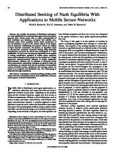
1. Introduction. In this paper we consider a fully distributed system, which consists of non cooperative nodes which can be modeled as a non cooperative game for Nash seeking. Let us consider a distributed system with N nodes or agents which interact with one another and each has a payoff/utility/reward to maximize. The decision or action of each node has an impact on the reward of the other nodes, which makes the problem challenging in general. In such systems each node has access to a numerical value of their utility/reward at each time. In such systems it might not be possible to have a bird’s eye view of the system as it is too complicated or is constantly changing. Let aj,k be the action of node j at time k and the numerical value of the utility of this node is given by r˜j,k . Where r˜j,k = rj (Sk , ak ) + ηj,k were ηj,k represents N ×N is the noise , rj : S × RN + −→ R is the payoff function of node j, Sk ∈ S ⊆ C state such that S is compact, ak = (a1,k , . . . , aN,k ) is the action vector containing actions of all nodes at time k. Figure 1.1 shows the system model where we have N interacting nodes. The rewards are interdependent as the nodes interact with one another. The only assumption that we can make here is the existence of a local solution. Each of these nodes j has access to the numerical value of their respective reward r˜j,k and it needs to implement a scheme to select an action aj,k such that its utility is maximized. The above scenario can be interpreted as an interactive game. In this paper we explore learning in such games which is synonymous with designing distributed iterative algorithms that converge to the Nash equilibrium. • Different approaches, mainly based on gradient descent or ascent method [3], have been developed to achieve a local optimum (or global optimum in some special cases, e.g. concavity of the payoff, etc.) of the distributed optimization problem. The method of gradient ascent is also called steepest ascent method, which starts at a point a0 and, as many times as needed, moves from ak to ak+1 by maximizing ∗ A preliminary work [20] (a conference paper of 5 pages) that focuses on the telecommunications application of some of the results without proofs has been presented at SPAWC 2012. All the theoretical results (i.e. theorems and proofs) are presented in this paper. The research of Ahmed Farhan Hanif and Djamal Zeghlache has received partial funding from the European Community’s Seventh Framework Programme (FP7/2007-2013) under grant agreement SACRA n 249060. † Institut Mines-T´ el´ ecom, T´ el´ ecom SudParis, RS2M Dept, France, ‡ Telecomm Dept, Ecole Superieure d’Electricite (Supelec), France. † {ahmedfarhan.hanif,djamal.zeghlache}@it-sudparis.eu, ‡ {hamidou.tembine,mohamad.assaad}@supelec.fr.

1

x1

r˜1,k a1,k

.. . xj

r˜j,k aj,k

.. . xN

r˜N,k aN,k

Rx1 Dynamic Environment RxA3 j S {rj (.)}

action state payoff function

Rx4

Fig. 1.1. Nodes interacting with each other through a dynamic environment

along the line extending from ak in the direction of ∇rj (Sk , ak ), the local downhill gradient. This gives the iterative scheme aj,k+1 = aj,k + λk ∇rj (Sk , ak ) where λk > 0 is a learning rate/step size. For the applicability of the above algorithm it is necessary to have access to the value of ∇rj (.) at each time k. The action can be positive and upper bounded by a certain maximum value aj,max > 0 for some engineering applications. Thus, the component aj,k needs to be projected in the domain [0, aj,max ]. This leads to a projected gradient descent or ascent algorithms: aj,k+1 = proj[0,aj,max ] {aj,k + λk ∇rj (Sk , ak )} where proj denotes the projection operator. At each time k, node j needs to observe/compute the gradient term ∇rj (Sk , ak ). Use of the aforementioned gradient based method requires the knowledge of (i) the system state, (ii) the actions of others and their states and or (iii) the mathematical structure (closed form expression) of the payoff function. As we can see, it will be difficult for node j to compute the gradient if the expression for the payoff function rj (.) is unknown and/or if the states and actions of other nodes are not observed as rj (.) depends on the actions and states of others. • There are several methods for Nash equilibrium seeking where we only have access to the numerical value of the function at each time and not its gradient (e.g. Complex functions which cannot be differentiated or unknown functions). Some of them are detailed below. The stochastic gradient ascent proposes to feedback the numerical value of gradient of reward function ∇rj of node j (which can be noisy) to itself. This supposes in advance that a noisy gradient can be computed or is available at each node. Note that if the numerical value of the gradients of the payoffs are not known by the players, this scheme cannot be used. In [4] projected stochastic gradient based algorithm is presented. A distributed asynchronous stochastic gradient optimization algorithms is presented in [5]. Incremental Sub-gradient Methods for Non-differentiable Optimization are discussed in [6]. A distributed Optimization algorithms for sensor networks is presented in [7]. Interested readers are referred to a survey by Bertsekas [8] on Incremental gradient, subgradient, and proximal methods for convex optimization. In [9] the authors present Stochastic extremum seeking with applications to mobile sensor networks. • Krstic et.al. in recent years have contributed greatly to the field of non-model 2

based extremum seeking. In [1], the authors propose a Nash seeking algorithm for games with continuous action spaces. They proposed a fully distributed learning algorithm and requires only a measurement of the numerical value of the payoff. Their scheme is based on sinus perturbation (i.e. deterministic perturbation instead of stochastic perturbation) of the payoff function in continuous time. However, discrete time learning scheme with sinus perturbations is not examined in [1]. In [10] extremum seeking algorithm with sinusoidal perturbations for non-model based systems has been extended and modified to the case of i.i.d. noisy measurements and vanishing sinus perturbation, almost sure convergence to equilibrium is proved. Sinus perturbation based extremum seeking for state independent noisy measurement is presented in [11]. Kristic et al. [2] have recently extended Nash seeking scheme to stochastic non-sinusoidal perturbations. In this paper we extend the work in [1] to the case of stochastic state dependent payoff functions, and use deterministic perturbations for Nash seeking. One can see easily the difference between this paper and the previous existing works [10][11]. In these works, the noise ηj associated with the measurement is i.i.d. which does not hold in practice especially in engineering application where the noise is in general time correlated. In our case, we consider a stochastic state dependent payoff function and our problem can be written in Robbins-Monro form with a Markovian (correlated) noise given by ηj = rj (S, a) − ES [rj (S, a)] (this will become clearer in the next sections), i.e. the associated noise is stochastic state dependent which is different from the case of i.i.d. noise. Although stochastic estimation techniques do estimate the gradient but they introduce a level of uncertainty, to avoid this it is possible to introduce sinus perturbation instead of stochastic perturbation. This is particularly helpful when one node is trying to follow the actions of the other nodes in a certain application. 1.1. Contribution. In this paper, we propose a discrete time learning algorithm, using sinus perturbation, for continuous action games where each node has only a numerical realization of the payoff at each time. We therefore extend the classical Nash Seeking with sinus perturbation method [1] to the case of discrete time and stochastic state-dependent payoff functions. We prove that our algorithm converges locally to a state independent Nash equilibrium in Theorem 1 for vanishing step size and provide an error bound in Theorem 2 for fixed step size. Note that since the payoff function may not necessarily be concave, finding a global optimum at affordable complexity can be difficult in general even in deterministic case (fixed state) and known closed-form expression of payoff. We also show the convergence time for the sinus framework in Corollary 1. In this paper we analyze and prove that the algorithm converges to a limiting ODE. We provide the convergence time and error bound between our discrete time algorithm and the ODE. The proof of the theorems are given in Appendix A. 1.2. Structure of the paper. The remainder of this paper is organized as follows. Section 2 provides the proposed distributed stochastic learning algorithm. The performance analysis of the proposed algorithm (convergence to ODE, error bounds) is presented in section 3. A numerical example with convergence plots is provided in section 4. Section 5 concludes the paper. Appendix contains the proofs. 1.3. Notations. We summarize some of the notations in Table 1.1. 2. Problem Formulation and Proposed Algorithm. Let there be N distributed nodes each with a payoff function represented by rj (Sk , aj,k , a−j,k ) at time 3

Table 1.1 Summary of Notations

Symbol N Aj S rj aj,k a−j,k E ∇

Meaning set of nodes set of choices of node j, state space payoff of node j decision of j at time k (aj ′ ,k )j ′ 6=j expectation operator gradient operator

k which is used to formulate the following robust problems: sup ES rj (S, aj , a−j ) ∀ j ∈ N , {1, . . . , N }

(2.1)

aj ≥0

A solution to the problem (2.1) is called state-independent equilibrium solution. Q Definition 1 (Nash Equilibrium (state-independent)). a∗ = (a∗j , a∗−j ) ∈ j ′ Aj ′ is a (state-independent) Nash equilibrium point if ES rj (S, a∗j , a∗−j ) ≥ ES rj (S, a′j , a∗−j ), ∀a′j ∈ Aj , a′j 6= a∗j

(2.2)

where ES denotes the mathematical expectation over the state. Definition 2 (Nash Equilibrium (state-dependent)). We define a state-dependent strategy a ˜j of a node j as a mapping from S to the action space Aj . The set of statedependent strategy is PG j : {˜ aj : S −→ Aj , S 7−→ a ˜j (S) ∈ Aj }. ˜∗−j ) ∈ a ˜∗ = (˜ a∗j , a

Y i

PG i

is a (state-dependent) Nash equilibrium point if ˜∗−j (S)) ≥ ES rj (S, a ˜∗−j (S)), ∀˜ ES rj (S, a ˜∗j (S), a ˜′j (S), a a′j ∈ PG j

(2.3)

Here we define a := (aj , a−j ) Assuming that node j has access to it’s realized payoff at each time k but the closed-form expression of rj (Sk , aj,k , a−j,k ) is unknown to node j. A solution to the above problem is a state-independent equilibrium in the sense no node has incentive to change its action when the other nodes keep their choice. It is well-known that equilibria can be different than global optima, the gap between the worse equilibrium and the global maximizer is captured by the so-called price of anarchy. Thus solution obtained by our method can be suboptimal with respect to maximizing the sum of all the payoffs. We study the local stability of the stochastic algorithm. The robust game is defined as follows: N is the set of nodes, Aj is the action N ×N space of node ; and Q j. S is the state space of the whole system, where S ⊆ C rj : S × j ′ ∈N Aj ′ −→ R is a smooth function. It should be mentioned here for clarity that the decisions are taken in a decentralized fashion by each node. Let us continue by stating that N is the set of nodes, Aj is the action space Q of node j, S is the state space of the whole system, where S ⊆ CN ×N and rj : S × j ′ ∈N Aj ′ −→ R. 4

Games with uncertain payoffs are called robust games. Since state can be stochastic, we get a robust game. Here we will focus on the analysis of the so-called expected robust game i.e (N , Aj , ES rj (S, .)). A (state-independent) Nash equilibrium point [14] of the above robust game is a strategy profile such that no node can improve its payoff by unilateral deviation, see Definition 1 and Definition 2. Since the current state is not observed by the nodes, it will be difficult to implement state-dependent strategy. Our goal is to design a learning algorithm for a state-independent equilibrium given in Definition 1. In what follows we assume that we are in a setting where the above problem has at least one isolated state-independent equilibrium solution. More details on existence of equilibria can be found in Theorem 3 in [15]. 2.1. Learning algorithm. Suppose that each node j is able to observe a numerical value r˜j,k of the function rj (Sk , ak ) at time k, where ak = (aj,k , a−j,k ) is the action of node j at time k. a ˆj,k is an intermediary variable. aj , Ωj φj represent the amplitude frequency and phase of the sinus perturbation signal given by bj sin(Ωj kˆ + φj ), r˜j,k+1 represents the payoff at time k + 1. The learning algorithm is presented in Algorithm 1 and is explained below. At each time instant k, each node updates its action aj,k , by adding the sinus perturbation i.e. bj sin(Ωj kˆ + φj ) to the intermediary variable a ˆj,k using equation (2.4), and makes the action using aj,k . Then, each node gets a realization of the payoff r˜j,k+1 from the dynamic environment at time k + 1 which is used to compute a ˆj,k+1 using equation (2.5). The action aj,k+1 is then updated using equation (2.4). This procedure is repeated for the window T . The algorithm is in discrete time and is given by aj,k = a ˆj,k + bj sin(Ωj kˆ + φj ) rj,k+1 a ˆj,k+1 = a ˆj,k + λk zj bj sin(Ωj kˆ + φj )˜

(2.4) (2.5)

Pk where kˆ := k′ =1 λk′ , Ωj 6= Ωj ′ , Ωj ′ + Ωj 6= Ωj ′′ ∀j, j ′ , j ′′ . For almost sure convergence, it is usual to consider vanishing step-size or learn1 ing rate such as λk = k+1 . However, constant learning rate λk = λ could be more appropriate in some regime. The parameter φj belongs to [0, 2π]∀ j, k ∈ Z+ Algorithm 1 Distributed learning algorithm 1: Each node j, initialize a ˆj,0 and transmit 2: Repeat 3: Calculate action aj,k according to Equation (2.4) 4: Perform action aj,k 5: Observe r ˜j,k 6: Update a ˆj,k+1 using Equation (2.5) 7: until horizon T Remark 1 (Learning Scheme in Discrete Time). As we will prove in subsection 3.1, the difference equation (2.4) can be seen as a discretized version of the learning scheme presented in [1]. But it is for games with state-dependent payoff functions i.e., robust games. It should be mentioned here for clarity that the action aj,k of each node j is scalar. 2.2. Interpretation of the proposed algorithm. In some sense our algorithm is trying to estimate the gradient of the function rj (.), but we don’t have access to 5

the function but just its numerical value. The following equation clearly illustrated the significance of each variable and constant in the algorithm. Perturbation Frequency

Learning Rate

a ˆj,k+1 = a ˆj,k | {z } |{z} New Value

Old Value

z}|{ + λk

zj |{z}

sin(

bj |{z}

z}|{ Ωj

New Reward

kˆ +

Growth Perturbation Amplitude Rate

z }| {

) r˜j,k+1 (2.6)

φj |{z} Perturbation Phase

The learning rate λk can be constant or variable depending on the requirement for the algorithm and system limitations. Perturbation amplitude bj > 0 is a small number. zj > is also a small value which can be varied for fine tuning. Rewriting the above equation we get a ˆj,k+1 − a ˆj,k rj,k+1 = zj bj sin(Ωj kˆ + φj )˜ λk

(2.7)

For vanishing step size as k −→ ∞ λk −→ 0 and the trajectory of the above algorithm coincides with the trajectory of the ODE in equation (3.11) 3. Main results. In this section we present the convergence results as introduced in the contribution section. 1 We introduce the following assumptions that will be used Pstep by stepP. 2 Assumption 1 (A1: Vanishing learning rate). λk > 0, k |λk | < k λk = ∞, ∞. There exists C0 > 0 such that P (supk k ak k< C0 ) = 1. The reason P for A1 is that λk represents the step size of the algorithm. So the sum over all k λk = ∞ as it P needs to traverse over all discrete time. The condition k |λk |2 < ∞ ensures bound for the cumulative noise error. This last assumption is for a local stability analysis. 1 Assumption 2 (A2: Constant learning rate). λt = λ > 0, supt [Ekat k2 ] 2 < +∞ and kat k2 is uniformly integrable. Assumption 3 (A3:Existence of a local maximizer). ES a∗j

∂rj (S,a∗ ) ∂aj

∂ 2 rj (S,a∗ ) ∂a2j ES rj (S, aj , a∗−j )

= 0, ES

0. These two conditions tell us that is a local maximizer of aj −→ where a∗−j = (a∗1 , . . . , a∗j−1 , a∗j+1 , . . . , a∗t ). Assumption 4 (A4: Diagonal Dominance). the  expected payoff a Hessian  2 has  P ∂ rj (S,a∗ ) ∂ 2 rj (S,a∗ ) that is diagonally dominant at a∗ , i.e., ES − > E S j ′ 6=j ∂aj ∂aj′ ∂a2j ∗ 0. Note that A4 implies that the Hessian of the expected payoff is invertible at a . This assumption is weaker compared to the classical extremum seeking algorithm because the Hessian of rj (S, a∗ ) does not need to be invertible for each S. We assume S 7−→ rj (S, a) is integrable with respect to S so that the expectation ES rj (S, a) is finite. 3.1. Convergence to ODE.

Stochastic approximation. First we need to show that our proposed algorithm converges to the respective ODE almost surely. We will use a dynamical system viewpoint and stochastic approximation method to analyze our learning algorithm. The idea consists of finding the asymptotic pseudo-trajectory of the algorithm via ordinary differential equation (ODE). To do so, we use the framework initiated by 1 We

do not use A1 and A2 simultaneously. 6


0 and ǫ¯, ¯bj such that, for all ǫ ∈ (0, ¯ǫ) and bj ∈ (0, ¯bj ), if the initial gap is ∆0 (which is small) then for all time t, ∆t ≤ y1,t

(3.7)

where ´ ´ e−mt y1,t , M ∆0 + O(ǫ + max b3j ) j

(3.8)

Proof. [Sketch of Proof of Theorem 3] Local stability proof of Theorem 3 follows the steps in [13]. From the above equation it is clear that as time goes to infinity the first term in y1,t bound vanishes exponentially and the error is bounded by the amplitude of the sinus perturbation i.e. O(ǫ + maxj b3j ). This means that the solution of ODE converges locally exponentially to the state-independent equilibrium action a∗ provided the initial solution is relatively close. Definition 3 (ǫ−Nash equilibrium payoff point). An ǫ−Nash equilibrium point in state-independent strategy is a strategy profile such that no node can improve its payoff more than ǫ by unilateral deviation. Definition 4 (ǫ−close Nash equilibrium strategy point). An ǫ−close Nash equilibrium point in state-independent strategy is a strategy profile such that the Euclidean distance to a Nash equilibrium is less than ǫ. A ǫ−close Nash equilibrium point is an approximate Nash point with a precision at most ǫ. It is not difficult to see that for Lipschitz continuous payoff functions, an ǫ−close Nash equilibrium is an Lǫ−Nash equilibrium point where L is the Lipschitz constant. Next corollary shows that one can get an ǫ−close Nash equilibrium in finite time. Corollary 1 (Convergence Time). Assume A3-A4 and Remark 3,4 holds. Then, the ODE reaches a (2ǫ + maxj b3j )−close to a Nash equilibrium in at most ´

∆0 M 1 T time units where T = m ´ log( ǫ ) Proof. [Sketch of Proof for Corollary 1] The proof follows from the inequality (3.7) in Theorem 3. Corollary 2 (Convergence to the ODE). Under Assumption A1, A3, and A4,

8

˜t − a∗ k≤ y1,t + y2,t where the following inequality holds almost surely: k a y2,t , CT (λt+k + L

X

k′ ≥0

λ2t+k′ ) + sup kδt,t+k′ k

(3.9)

k′ ≥0

˜t − a∗ k≤k Proof. [Proof of Corollary 2] The proof uses the triangle inequality k a ˜t − at k + k at − a∗ k . By Theorem 1, one gets k a ˜t − at k≤ y1,t and by Theorem 3, a one has k at − a∗ k≤ y2,t Combining together, one arrives at the announced result. Then constants in equation (3.8) and (3.9) depends on the number of players and the dimension of the action space. 3.2. Convergence of the stochastic ODE. In this subsection we study the stochastic ODE given by aj,t = a ˆj,t + bj sin(Ωj t + φj ) d a ˆj,t = zj bj sin(Ωj t + φj )˜ rj,t dt

(3.10) (3.11)

where rj,t is the realization of the state-dependent payoff rj (St , at ) at time t. We assume the state process is ergodic so that, 1 T −→∞ T lim

Z

T

1 T −→∞ T

µj (t)rj (St , at ) dt = lim

0

Z

T

µj (t)ES rj (S, at ) dt

0

In particular the asymptotic drift of the deterministic ODE and the stochastic ODE are the same. Hence, the following theorem follows: Theorem 4 (Almost sure exponential stability). The stochastic algorithm 1 converges asymptotically almost surely to the stochastic ODE in equation (3.11) i.e. ˜t − a∗ k≤ y1,t + y2,t ) = 1 a.s. P (k a Since the state process is ergodic, we can apply the stochastic averaging theorem from [2] to get the announced result. 4. Numerical Example: A Generic Wireless Network with Interference. Even though the distributed optimization problem, considered in this paper, and the developed approach are general and can be used in many application domains. As an application of the above framework, we will consider the problem of power control in wireless networks in order to better illustrate our contribution. Consider an interference channel composed of N transmit receiver pairs as shown in Figure 4.1. Each transmitter communicates with its corresponding receiver and incurs an interference on the other receivers. Each receiver feeds back a numerical value of the payoff γ˜j (H, p) to its corresponding transmitter. The problem is composed of transmitter-receiver pairs; all of them use the same frequency and thus generate interference onto each other. Each transmitter-receiver pair has therefore its own payoff/reward/utility function that depends necessarily on the interference exerted by the other pairs/nodes. Since the wireless channel is time varying as well as the interference, the objective is necessarily to optimize in the longrun (e.g. average) the payoff functions of all the nodes. The payoff function of node j at time k is denoted by rj (Hk , pk ) where Hk := [hk (i, j)] represents an N × N matrix containing channel coefficients at time k, hk (i, j) represents the channel coefficient 9

between transmitter i and receiver j (where (i, j) ∈ N 2 ) and pk represents the vector containing transmit powers of N transmit-receive nodes. The most common technique used to obtain a local maximum of the nodes’ payoff functions is the gradient based descent or ascent method. Remark 2. Table 4.1 Equivalent Notations for Wireless

General r˜j,k aj,k sjj ′ ,k

Application γ˜j,k pj,k gjj ′ ,k

Description utility/payoff of transmitter j at time k action/power of transmitter j at time k state/channel gain between transmitter j and receiver j ′ at time k

γ˜1 g11

T x1

Rx1 1

g j1 .. .

gN N

T xN

g1

j

.. .

gNj

g 1N

γ˜N

gN

γ˜j gjj

gj

N

RxN

Fig. 4.1. Interference Channel Model

In section 3, we proved that our proposed algorithm converges to p∗ for any type of payoff functions which satisfies the assumptions in section 3.1. In order to show numerically that our algorithm converges to p∗ , we run our algorithm for a simple payoff function. In parallel, we obtain analytically the Nash equilibrium p∗ and compare the convergence point of our algorithm to p∗ . We therefore choose a simple payoff function for which p∗ can be obtained analytically. The payoff function of node j at time k has then the following form:

γ˜j (Hk , pk ) =

ω |{z}

log(1 +

bandwidth |

σ2

p g P j,k jj,k )− κpj,k + j ′ 6=j pj ′ ,k gj ′ j,k | {z } {z } constraint on powers Rate

where ω represents the bandwidth available for transmission. The above payoff function γ˜j (Hk , pk ) consists of log of (1+SIN R) of user j and the unit cost of transmission is κ. It is assumed that a used doesn’t know the structure function γ˜j (.) or the law of the channel state. For the above payoff function to ensure the assumption A3-A4 10

P and Remark 3,4 we need to satisfy the condition E|hjj |2 ≥ E j ′ 6=j |hj ′ j |2 . Please see appendix for more details. The problem here is to maximize the payoff function γ˜j (H, p) which is stated as follows: find p∗ such that for each user j ∈ N , satisfies p∗j ∈ arg maxpj ≥0 E˜ γj (H, p∗1 , . . . , p∗j−1 , pj , p∗j+1 , . . . , p∗N ). Note that when gjj = 0 then the payoff of user j is negative and the minimum power p∗j = 0 is a solution to the above problem. For the remaining, we assume that |hjj |2 = gjj > 0. The channel hj,j ′ is time varying and is generated using an independent and 2 identically distributed complex gaussian channel model with variance σjj ′ such that ′ σjj = 1 σjj ′ = 0.1, j 6= j. The thermal noise is assumed to be a zero mean gaussian with variance σ 2 such that σ 2 = 1. We consider the following simulation settings with N = 2 for the above wireless model: k1 = 0.9, k2 = 0.9, φ1 = 0, φ2 = 0,Ω1 = 0.9, Ω2 = 1, b1 = 0.9, b2 = 0.9. The numerical setting could be tuned in order to make the convergence slower or faster with some other tradeoff. Due to space limitations further discussion on how to select these parameters has been omitted. p1,0 and p2,0 represent the starting points of the algorithm which are initialized as p1,0 = p∗1 + 10 and p2,0 = p∗2 + 10. κ = 2 is the penalty for interference, ω = 10 is the bandwidth and the variance of noise is normalized. Figure 4.2 represents the average transmit power trajectories of the algorithm for two nodes. The dotted line represents p∗ . As can be seen from the plots that the system converges to p∗ where p∗j = 3.9604, j ∈ {1, 2}. Realtime

Averaged

50

35 User

User

User2

User2

1

45

1

30 40 25

35

30 Power

Power

20 25

15 20

15

10

10 5 5

0

0

1000

2000 3000 Time

4000

0

5000

0

1000

2000 3000 Time

4000

5000

Fig. 4.2. Power evolution (discrete time)

The example we discussed is only one of the possible types of applications where our proposed algorithm can be implemented. 11

Realtime

Averaged

20

15 User1

User1

User2

User2

10

10

0 5

Reward

Reward

−10 0

−20 −5 −30

−10

−40

−50

0

1000

2000 3000 Time

4000

−15

5000

0

1000

2000 3000 Time

4000

5000

Fig. 4.3. Payoff evolution (discrete time)

Consider for example the following payoffs: q1 (.) = goodput(.) and q2 (.) = P(goodput(.) < η) where η is a small value and P(.) stands for probability. Goodput represents the ratio of correctly received information bits vs the number of transmitter bits. In wireless communications the channel is constantly changing due to various physical phenomenon and interference from other sources and changes in the environment. It is hard to have a closed form expression for q1 (.) due to complexity of the transmitter, receiver and unknown parameters. In practice, at each time k, the receiver has therefore a numerical value of goodput(.) but no closed form expression for rate/goodput is available especially for advanced coding scheme (e.g. turbo code, etc.). q2 (.) represents an outage probability for which also depends on the goodput, the gradient for q2 (.) is notoriously hard to compute without channel and interference statistics knowledge (probability distribution function) and closed form expression of goodput(.). Our scheme can be particularly helpful in such scenarios. The price/design parameter κ inside the reward function can be tuned such that the solution of the distributed robust extremum coincides with a global optimizer of the system designer. The κ can be same for all nodes or each node can have its own κj . Let a∗g represent the optimal action or set of actions to be performed by each node to maximize their respective utilities. It is possible to set κ such that the following equation is satisfied.a(κ) = a∗g . κ could represent a scalar or a vector depending on the system size and the application. To be able to effectively make a(κ) equal to a∗ we need to have enough degrees of freedom in the system. However this type of tuning is not true in general. 5. Concluding remarks. 12

Work Presented: In this paper we have presented a Nash seeking algorithm which is able to find the local minima using just the numerical value of the stochastic state dependent payoff function at each discrete time sample. We proved the convergence of our algorithm to a limiting ODE. We have provided as well the error bound for the algorithm and the convergence time to be in a close neighborhood of the Nash equilibrium. A numerical example for a generic wireless network is provided for illustration. The convergence bounds achieved by our method are dependent on the step size and the perturbation amplitude. New Class of Functions: In this work we introduced a new class of state dependent payoff functions rj (S, a) which are inspired from wireless systems applications. But these kind of functions are more general and appear in other application areas. Achievable Bounds: As it is clear from results in Theorem 1 that convergence depends on an exponential term and the amplitude of the sinus perturbation. As amplitude becomes smaller, the error bound also vanishes. In contrast the standard stochastic subgradient method only depend on the step size. Global Analysis: All the work considered in this paper including Krstic et.al. consider local stability. Our work is an extension of their work and works for local stability. The future work will focus on the extension to the case of Global Stability of Nash equilibrium for both deterministic and stochastic payoff functions. Multidimensional Aspect: The presented work has been studied for scalar reward and scalar action by each node. Scalar scenario has several applications to wireless (as in the aforementioned example) and sensor networks and numerous examples can be considered. A possible extension to this work could be in the direction of vector actions where each users is able to perform multiple actions based on multiple rewards. Appendix A. Convergence Theorems. A.1. Variable Step Size: Proof of Theorem 1. The Theorem 1 states that Under Assumption A1, the learning algorithm converges almost surely to the trajectory of a non-autonomous system given by d a ˆj,t = zj bj sin(Ωj t + φj )ES (rj (S, at )) dt aj,t = a ˆj,t + bj sin(Ωj t + φj ) The proof follows in several steps. • The first step provides conditions for Lipschitz continuity of the expected payoff which is given in Lemma 1. From Lemma 2 we have that ∀j, t, fj (t, a) , bj zj sin(Ωj t + φj )ES rj (S, a), is Lipschitz over the domain D • Second step: the learning rates are chosen such that they satisfy assumption A1. • Third step: we check the noise conditions. Lemma 1. Let (S, a) 7−→ rj (S, a)∀S ∈ S, ∃ Lj,S such that (C1 ) : krj (S, a) − rj (S, a′ )k ≤ Lj,S ka − a′ k ∀(a, a′ ) ∈ A

(C2 ) : ES Lj,S < +∞

13

then the mapping a 7−→ ES rj (S, a) is Lipschitz with Lipschitz constant Lj = ES Lj,S Proof. [Proof of Lemma 1] Suppose that a 7−→ ES rj (S, a) is Lipschitz with Lipschitz constant Lj,S , then by Jensen’s inequality one has kES rj (S, a) − ES rj (S, a′ )k ≤ ES krj (S, a) − rj (S, a′ )k By condition C2 , ES Lj,S < +∞. Let Lj be ES Lj,S . Then kES rj (S, a) − ES rj (S, a′ )k ≤ Lj ka − a′ k This completes the proof. Remark 3. • Note that under C1 and C2 the expected payoff vector r = (rj )j∈N is Lipschitz ˜ = maxj Lj , continuous with L • If S is a compact set and S 7−→ Lj,S is continuous then a 7−→ ES rj (S, a) is Lipschitz [In particular, the condition C2 is not needed] We shall prove the above remark by Reductio ad absurdum. To prove the second statement of Remark 3 we use compactness and continuity argument. We start from Bolzano–Wierstrass theorem which states that. For any k, any continuous map x 7−→ f (k, a) over a compact set D has at least one maximum, i.e., sup f (k, a) = maxa∈D f (k, a) < ∞. The proof of this statement can be easily done by contradiction. Suppose sup f (k, a) = ∞. Then there exists a sequence (al )l such that al ∈ D but f (k, al ) −→ ∞ as l goes to infinity. This is impossible because D is compact which implies that f (k, D) = {f (k, a) |a ∈ D} is bounded by continuity. Since S is compact and S 7−→ LS is continuous, supS∈S LS is also finite. Remark 4. If rj (S, a) is continuously differentiable with the respect to a then it is sufficient to check the expectation of the gradient is bounded (in norm). if S is in Euclidean Space • rj is differentiable w.r.t a • rj (S, a), ∇a rj (S, a) are continuous in S • rj (S, a), ∇a rj (S, a) are absolutely integrable in S and ES rj (S, a) is continuous in a. then E[∇a rj (S, a)] = ∇a E[rj (S, a)] which can be written as Z

S

∇a rj (S, a)γ(dS) = ∇a

Z

rj (S, a)γ(dS)

S

where γ is the measure of S state space. For more details on the above conditions please refer to [19]. Since fj is a function of time and the actions of nodes, we need a uniform Lipschitz condition on fj . We have |fj (t, a) − fj (t, a′ )| ≤ bj zj | sin(Ωj t + φ)| [kES rj (S, a) − ES rj (S, a′ )k] But one has | sin(.)| ≤ 1. Hence, |fj (t, a) − fj (t, a′ )| ≤ bj zj [kES rj (S, a) − ES rj (S, a′ )k] 14

We use Lemma 1, |fj (t, a) − fj (t, a′ )| ≤ bj zj Lj ka − a′ k This implies that the Lipschitz constant of fj is less than the one of rj times the factor bj zj . Finally, we check the noise conditions. The recursion equation is given by aj,k+1 = aj,k + λk [fj (k, ak ) + Mj,k+1 ] where Mj,k+1 is a martingale difference sequence. By definition the martingale sequence for the algorithm is given as rj,k+1 − ES [˜ rj,k+1 (S, ak+1 )]] Mj,k+1 , zj bj sin(Ωj kˆ + φj ) [˜ which satisfied the condition E[Mk+1 |Fk ] = 0 for k ≥ 0 almost surely (a.s.) Lemma 2. If ak ∈ D then the martingale is square-integrable with E[kMk+1 k2 |Fk ] ≤ c´(1 + kak k2 ) ∀k Proof. [Proof of Lemma 2] Let r˜j,k+1 be the realization the payoff at time k + 1. The expected value of this random variable can be bounded above the norm of ak . rj,k+1 − ES [˜ rj,k+1 (S, ak+1 )]) Mj,k+1 = zj bj sin(Ωj kˆ + φj )(˜ rj,k+1 − ES [˜ rj,k+1 (S, ak+1 )]k) kMj,k+1 k ≤ |zj ||bj ||(sin(Ωj kˆ + φj )|k˜ ≤ zj bj (k˜ rj,k+1 k + kES [˜ rj,k+1 (S, ak+1 )]k) ≤ zj bj (k˜ rj,k+1 k + ES k˜ rj,k+1 (S, ak+1 )k)

≤ zb(k˜ rj,k+1 k + ES k˜ rj,k+1 (S, ak+1 )k)

Where | sin(.)| ≤ 1, z , max |zj |, b , max |bj |, k˜ rj,k+1 k is bounded because of the Lipschitz condition as mentioned in C1 , which is shown below. krj (S, ak ) − rj (S, 0)k ≤ Lj,S kak − 0k ∀(ak ) ∈ A

(A.1)

krj (S, ak )k ≤ krj (S, 0)k + Lj,S kak k ≤ β1,S + Lj,S kak k

Where β1,S , krj (S, 0)k. The above equations A.1 show that krj (S, a)k is bounded by β1,S + Lj,S kak. By taking expectation of the above set of inequalities we get. ES krj (S, ak )k ≤ ES krj (S, 0)k + ES Lj,S kak k ≤ Lj kak k + ES krj (S, 0)k

(A.2)

≤ Lj kak k + β2

Where β2 , ES krj (S, 0), Lj , ES Lj,S . The above set of inequalities A.2 show that ES krj (S, a)k is bounded. Combining the results of inequalities in A.1 A.2 we can get 15

kMj,k+1 k2 ≤ z 2 b2 (β1,S + Lj,S kak k + Lj kak k + β2 )2 ≤ 2z 2 b2 ((β1,S + β2 )2 + (Lj,S + Lj )2 kak k2 ) 2 ≤ 4z 2 b2 (β1,S + β22 + (L2j,S + L2j )kak k2 )

Taking ES over the above inequalities we get: 2 + β22 + (ES L2j,S + L2j )kak k2 ) ES kMj,k+1 k2 ≤ 4z 2 b2 (ES β1,S ` j kak k2 ) ≤ 4z 2 b2 (β + L

≤ c´(1 + kak k2 )

` j , ES L2 + L2 , β , ES β 2 + β 2 and c´ ≥ 4z 2 b2 (β + L `j) Where L 2 j j,S 1,S This completes the proof. We now combine the above three steps to derive almost sure convergence to an ODE. To do so, we interpolate the stochastic process ak (an affine interpolation) in order to get a continuous time process following the lines of Borkar [12] Chapter 2 Lemma 1. The gap between the solution of the non-autonomous differential equation given by d at = f (t, at ) dt and the interpolated process vanishes almost surely for asymptotic interval of length T > 0. lim

sup

t−→∞ q∈[t,t+T ]

k˜ aq − a∗q k = 0 a.s.

In order to calculate the bound we need to define a few terms which are helpful in obtaining a compact form of the bound. sup t∈[tk ,tk +T ]

k˜ a(t) − atk (t)k ≤ KT,t eLT + CT λt+k´ = CT (λt+k´ + L

X

λ2t+k´ )

´ k≥0

+ sup kδt,t+k´ k ´ k≥0

where KT,t , CT L

X

´ k≥0

λ2t+k´ + sup kδt,t+k´ k ´ k≥0

δt,t+k´ , ξt+k´ − ξt ξt ,

t−1 X

λm Mm+1

m=0

CT , kr(0)k + L(C0 + kr(0)kT )eLT < ∞ !

P sup kak´ k < C0 ´ k

=1

then we conclude by discrete adaptation of Lemma 1 in Borkar [12]. 16

A.2. Fixed Step Size: Proof of Theorem 2. Theorem 2 states that Under Assumption A2, the learning algorithm converges in distribution to the trajectory of a non-autonomous system given by

d a ˆj,t = zj bj sin(Ωj t + φj )ES (rj (S, at )) dt aj,t = a ˆj,t + bj sin(Ωj t + φj ) ˜ ˆt be the interpolated version the trajectory of our algorithm Proposition 1. Let a ˜ˆt ˆt is the trajectory of the the ODE at time t. Under assumption A2 a at time t a ˆt as step size vanishes. converges to a √ 1 ˜ ˆt − a ˆt k2 ] 2 = C˜T λ E sup [ka t∈[0,T ]

Proposition 1 implies theorem 2. Proof. [Proof of Proposition 1] To prove the above proposition we start with a fixed step size λ > 0. Pt • Time Scale. Tt = k=1 λ = tλ, for t ≥ 0 P Pt−1 • The cumulative noise at iteration t ξt = t−1 k=1 λMk+1 = λ k=1 Mk+1 • Define the (affine) interpolated process from {ˆ a}k≥0 rewritten as a ˆj,k+1 = a ˆj,k + λ(fj (k, a ˆk ) + Mk+1 ). The advantage of the interpolated process is that it is defined for any con˜ˆj,t = a tinuous time by concatenation. The affine interpolation writes a ˆj,k + t−Tk ( λ )(ˆ aj,k+1 − a ˆj,k ) if t ∈ [kλ, (k + 1)λ[ which is now in continuous time. Note that constant learning rate or constant step size λt = λ is suitable for many practical scenarios. It is used for example in numerical analysis: Euler-s Scheme (1st Order), Runge Kutta’s scheme (4th Order), etc. Our algorithm writes

(∗∗)



a ˆj,k+1 aj,k+1

= =

a ˆj,k + λ(bj zj sin(kˆt Ωj + φj ))˜ rj,t ˆ a ˆj,k + (bj sin(kt Ωj + φj ))

where λ is a constant learning rate, our aim is to analyze (∗∗) asymptotically when λ is very small. In order to prove an asymptotic pseudo-trajectory result for constant learning rate, we need additional assumptions of the sequence generated by the powers. The key additional assumption is the uniform integrability of that process. We need the conditions C1 C2 , which translate into - From Remark 4: gradient of the expectation of payoff is bounded - From Lemma 2: Square of the martingale is bounded - Uniform Integrability of rj (S, a) ˆ˙ t = f (t, a ˆt ) starting from a ˆ t ˆt is the solution of a and a ⌊λ⌋

17

˜ ˆTt+m = a

m X

k=1 λ(fj (⌊

˜ˆT ˜ ˆTt+k − a ) (a t+k−1 | {z }

Tt+k−1 λ

⌋,ˆ a

⌊

Tt+k−1 )+Mk+1 ) ⌋ λ

˜ ˆ⌊ Tt+k−1 ⌋ +a λ

˜ ˆTt+m = a

m X

(Tt+k − Tt+k−1 )fj (⌊

k=1 m X

+

Tt+k−1 ˆ⌊ Tt+k−1 ⌋ ) ⌋, a λ λ

˜ˆT λMt+k+1 + a t

k=1

˜ ˆTt+m = a

m Z X

Tt+k−1

+

˜ˆT λMt+k+1 + a t

fj (⌊

k=1 Tt+k m X

Tt+k−1 ˆ⌊ Tt+k−1 ⌋ )ds ⌋, a λ λ

k=1

˜ ˆTt+m = a

m Z X k=1

˜ ˆTt+m a

Tt+k−1

fj (⌊

Tt+k

Tt+k−1 ˆ⌊ Tt+k−1 ⌋ )ds ⌋, a λ λ

˜ˆT +(ξt+m − ξt ) + a t Z m X Tt+k−1 s ˜ ˆ⌊ λs ⌋ )ds fj (⌊ ⌋, a = λ Tt+k k=1

˜ˆT +(ξt+m − ξt ) + a t

Now we use Burkholder’s inequality which states the following: For an α > 0 there exists two constants c1 > 0 and c2 > 0 such that

c1 E[

t X

k=1

ˆk−1 k2 ]α/2 ≤ E[sup kˆ kˆ ak − a at k] m≥t

≤ c2 E[

c1 E[

t X

k=1

t X

k=1

ˆk−1 k2 ]α/2 kˆ ak − a

kˆ ηk − ηˆk−1 k2 ]α/2 ≤ E[sup kηk k] k≤t

≤ c2 E[ 18

t X

k=1

kˆ ηk − ηk k2 ]α/2

Take ηˆt = λ that

P

k≤m

kMt+k k2 and we use discrete Gronwall inequality which states ǫt+1 ≤ C + L ǫt+1 ≤ CeLλt

t X

λǫk

k=0

where ǫt > 0 ∀t ≥ 0 for ˜ ˆTt+k′ − a ˆTt+k′ k2 ]1/2 ǫk = E[ sup ka k′ ≤k

p p C = λT K1 1 + C02 + λK2 (1 + C02 ), L = maxj∈N ES [Lj,S ] for some K1 , K2 = c2 from the above we deduce that ˜ ˆTt+k′ − a ˆTt+k′ k2 ]1/2 ≤ E[ sup ka k′ ≤k

√

λCT

p K1 = max(c1 , c2 1 + C02 ) ˜ ˆTt+k′ − a ˆTt+k′ k2 ]1/2 is bounded and implies PropoThis shows that E[supk′ ≤k ka sition 1. When λ −→ 0 we have a weak √ convergence of the interpolated process to a solution of the ODE. The error gap is λCT which vanishes as λ −→ 0. Appendix B. Conditions for our Example. Following are some details about how to obtain a∗ for our application. gi,j , |hi,j |2 g¯i,j , Eg gi,j = Eg |hi,j |2 ∂γ (G,a∗ )

From remark 4 we can write EG j ∂aj equations we have the following matrix form. 

  a∗1 g¯1,1  a∗2   g¯2,1   ¯  a∗ =  .  , G = .  ..   .. a∗N

g¯N,1

g¯1,2 g¯2,2 .. .

··· ··· .. .

g¯N,2

···

=

∂ ∗ ∂aj EG γj (G, a )

  g¯1,N  g¯2,N    ¯= ..  , a  . 

g¯N,N

= 0. Solving N

 − σ2 − σ2    ..  . ω¯ gN,N 2 −σ λ ω¯ g1,1 λ ω¯ g2,2 λ

The above equation can be written in the compact form as ¯ −1 a ¯ a∗ = G

¯ should be invertible and all the elements in the vector a ¯ should be strictly G positive as they are a linear combination of power and gains which are positive. We can also write ω¯ gj,j > λσ 2 . For this example we can write 19

EG [gj,j ] >

X

j ′ 6=j

EG [gj,j ′ ] ∀j, j ′ 6= j

¯ is invertible. If this condition is satisfied then G As G is a matrix of random channel gains it is almost surely invertible. To show ¯ 6= 0 the invertibility of this matrix we just need to show that the det(G) REFERENCES [1] Frihauf, P; Krstic, M.; Basar, T.; , ”Nash Equilibrium Seeking in Noncooperative Games,” Automatic Control, IEEE Transactions on , vol.57, no.5, pp.1192-1207, May 2012. [2] S.-J. Liu and M. Krstic, Stochastic averaging in continuous time and its applications to extremum seeking, IEEE Trans. Automat. Control, 55 (2010), pp. 22352250. [3] Jan A. Snyman (2005). Practical Mathematical Optimization: An Introduction to Basic Optimization Theory and Classical and New Gradient-Based Algorithms. Springer Publishing. ISBN 0-387-24348-8 [4] P. Bianchi, J. Jakubowicz “On the Convergence of a Multi-Agent Projected Stochastic Gradient Algorithm,” to appear in IEEE Trans. on Automatic Control, Feb. 2013. [5] Tsitsiklis, J.; Bertsekas, D.; Athans, M.; , ”Distributed asynchronous deterministic and stochastic gradient optimization algorithms,” Automatic Control, IEEE Transactions on , vol.31, no.9, pp. 803- 812, Sep 1986 [6] A. Nedic and D. Bertsekas, Incremental Subgradient Methods for Nondifferentiable Optimization, SIAM Journal of Optimization, vol. 12, no. 1, pp. 109138, 2001. [7] M. Rabbat and R. Nowak, Distributed Optimization in Sensor Networks, in Proceedings of the 3rd international symposium on Information processing in sensor networks. ACM, 2004, pp. 2027. [8] D. P. Bertsekas, Incremental gradient, subgradient, and proximal methods for convex optimization: A survey, MIT, Cambridge, MA, LIDS Tech. Rep., 2010. [9] M. S. Stankovic and D. M. Stipanovic, Stochastic extremum seeking with applications to mobile sensor networks, in Proc. American Control Conference, 2009, pp. 56225627. [10] M. S. Stankovic’ and D. M. Stipanovic’. Extremum Seeking under Stochastic Noise and Applications to Mobile Sensors, Automatica, vol. 46, pp. 12431251, 2010. [11] M. S. Stankovic’, K. H. Johansson and D. M. Stipanovic’. Distributed Seeking of Nash Equilibria with Applications to Mobile Sensor Networks, IEEE Trans. Automatic Control, Vol. 57(4), pp. 904-919, 2012. [12] Vivek S. Borkar, Stochastic approximation: a dynamical systems viewpoint, 2008, http://www.tcs.tifr.res.in/∼borkar/trimROOT.pdf [13] Shu-Jun Liu, Miroslav Krstic, Stochastic Nash Equilibrium Seeking for Games with General Nonlinear Payoffs. SIAM J. Control and Optimization 49(4), 1659-1679 (2011). [14] Nash J.,Equilibrium points in n-person games, Proceedings of the National Academy of Sciences 36(1):48-49, 1950. [15] Michael R. Baye, Guoqiang Tian and Jianxin Zhou, Characterizations of the Existence of Equilibria in Games with Discontinuous and Non-Quasiconcave Payoffs, The Review of Economic Studies Vol. 60, No. 4 (Oct., 1993), pp. 935-948. [16] Herbert Robbins and Sutton Monro, A Stochastic Approximation Method, Annals of Mathematical Statistics 22, 3 (September 1951), pp. 400-407. [17] J. Kiefer and J. Wolfowitz, Stochastic Estimation of the Maximum of a Regression Function, Annals of Mathematical Statistics 23, 3 (September 1952), pp. 462-466. [18] Benaim, M. Dynamics of Stochastic Algorithms, In Seminaire de Probabilites XXXIII, J. Azema et. al., Eds. Lecture Notes in Mathematics 1709, Berlin: Springer, 1999. [19] L. Schwartz, Functionl Analysis, Courant Institute of Mathematical Sciences, New York University; 1st edition (1964) [20] Hanif, Ahmed Farhan; Tembine, Hamidou; Assaad, Mohamad; Zeghlache, Djamal; , ”Distributed stochastic learning for continuous power control in wireless networks,” Signal Processing Advances in Wireless Communications (SPAWC), 2012 IEEE 13th International Workshop on , vol., no., pp.199-203, 17-20 June 2012

20