for average aggregate computation on a wireless sensor network with dynamical .... information, the DRG algorithm constructs âgroupsâ each of which typically ...
On the Convergence of Distributed Random Grouping for Average Consensus on Sensor Networks with Time-varying Graphs Jen-Yeu Chen and Jianghai Hu Abstract— Dynamical connection graph changes are inherent in networks such as peer-to-peer networks, wireless ad hoc networks, and wireless sensor networks. Considering the influence of the frequent graph changes is thus essential for precisely assessing the performance of applications and algorithms on such networks. In this paper, we analyze the performance of an epidemic-like algorithm, DRG (Distributed Random Grouping), for average aggregate computation on a wireless sensor network with dynamical graph changes. Particularly, we derive the convergence criteria and the upper bounds on the running time of the DRG algorithm for a set of graphs that are individually disconnected but jointly connected in time. An effective technique for the computation of a key parameter in the derived bounds is also developed. Numerical results and an application extended from our analytical results to control the graph sequences are presented to exemplify our analysis.
I. I NTRODUCTION Dynamical graph changes are inherent in networks such as peer-to-peer networks, wireless ad hoc networks, and wireless sensor networks. Take the example of the wireless sensor networks, which have attracted tremendous research interests in the recent years. In a practical or even hostile environment, the connection graph of a sensor network may vary frequently in time due to various reasons. For instance, the communication links (edges of the graph) may fail for being interfered, jammed or obstructed; sensor nodes may be disabled or relocate in the field; to save energy, some sensor nodes may sleep or adjust their transmission ranges, thus altering the connection graph. Algorithms and protocols developed on these networks need to take this nature into consideration. In this setting, distributed and localized algorithms requiring no global data structure and centralized coordination are preferable for their scalability and robustness to the frequent graph changes [1], [2], [3], [4], [5], [6]. Although various distributed algorithms have been designed to work well on a time-varying graph, their performances are usually analyzed under the assumption of a fixed connection graph [2], [3], [4]. In this paper, as a particular example, we analyze the performance of a distributed randomized algorithm, namely, the DRG (Distributed Random Grouping) algorithm proposed in [2], for average aggregate computation on sensor networks with randomly changing graphs. The analysis techniques introduced in this paper can also be applied to other algorithms whose performances depend on the network connection graph. This work was partially supported by the National Science Foundation under Grant CNS-0643805. The authors are with the School of Electrical and Computer Engineering, Purdue University, USA. E-mail: {jenyeu,jianghai}@purdue.edu.
Average aggregate computation is an essential operation in sensor networks. One typical category of algorithms to compute the average aggregate is the tree-based algorithms [7], [8]. In these algorithms, sensor nodes’ values are gathered along an aggregation tree to the tree’s root, the sink node. The other class of algorithms is the epidemic-like algorithms, such as gossip and the DRG algorithm. Unlike tree-based approaches where only the sink node obtains the global average value, epidemic-like algorithms obtain an distributed average consensus among all sensor nodes. Distributed average consensus has been an important problem with many applications in distributed and parallel computing. Recently it also finds applications in the coordination of distributed dynamic systems and multi-agent systems [9], [10], [11], [12], as well as in distributed data fusion in sensor networks [2], [3], [4], [5]. In analyzing the performance of the proposed distributed schemes for average consensus, authors of [2], [3], [4] bound the running time of their schemes on fixed connected graphs. In [9] OlfatiSaber and Murray characterize the convergence speed of their scheme – over a set of possible directed graphs assumed to be balanced and strongly connected – by the minimal algebraic connectivity of the mirror (undirected) graph of each possible network graph. Authors of [5], [10], [11], [12] provide criteria for their schemes to converge on a dynamical changing graph which is possibly disconnected during some time period but do not characterize the convergence speed. Different from these works, the goal of this paper is to not only determine the convergence criteria but also bound the running time of the DRG algorithm on a randomly changing graph which especially could be disconnected all the time. This paper is organized as follows. In Section II we briefly introduce the DRG algorithm and review its performance on a fixed graph. Then in Section III and Section IV, we analyze the performance of the DRG algorithm on a network graph randomly switching among a set of individually disconnected but jointly connected graphs. Numerical results on four typical sets of such graphs are provided in Section V. An application based on our analytical results to optimize and control the sensors’ sleep/awake schedule is presented in section VI. Finally, we conclude our work in Section VII. II. D ISTRIBUTED
RANDOM GROUPING
We present in [2] a distributed, localized, and randomized algorithm called the Distributed Random Grouping (DRG) algorithm to compute the aggregate statistics such as average, sum or maximum among all sensor nodes’ measurements. The DRG algorithm is similar to the gossip algorithm [3],
[4] but with a better performance (shown in [2])—unlike the gossip algorithm which forms “pairs” of nodes to exchange information, the DRG algorithm constructs “groups” each of which typically includes more than two nodes to expedite the information mixing process. (Hence, in this paper, we focus on the DRG algorithm rather than the renowned gossip algorithm.) In the following, we will briefly describe the DRG algorithm, which will be the focus of this paper in a generalized setting of time-varying network graphs. Each sensor node i is associated with an initial observation or measurement value denoted by vi (0) ∈ R. The values over all nodes form a vector v(0). The goal is to compute (aggregate) functions such as the average, sum, max, min, etc of the entries of v(0) in a distributed manner. Throughout this paper we use vi (k) to denote the value of node i and v(k) = [v1 (k), v2 (k), . . .]T the value distribution vector after running the DRG algorithm for k rounds. The main idea of the DRG algorithm is as follows. In each round of the iteration, each node independently becomes a group leader with a probability pg and then invites its onehop neighbors to join its group by wireless broadcasting an invitation message1 . A neighbor who successfully2 receives the invitation message then join its group. Note that unlike the concept of a cluster in the sensor network literature, a group contains only the group leader and its one-hop neighbors. Several disjoint groups are thus formed over the network. Next, in each group, all members other than the group leader then send the leader their values so that the leader can compute the local aggregate (e.g., average in the group) and broadcast it back to the members to update their values. Since in each round, groups are formed at different places of the network, through this randomized process, the values of all nodes will diffuse and mix over the network and converge to the correct aggregate value asymptotically almost surely, provided that the graph is connected. DRG iterations stop when certain accuracy criteria are satisfied. A high-level description of a round (iteration) of the DRG algorithm to compute the average aggregate, is shown in Fig. 1. Aggregates other than the average can be obtained by an easy modification of this algorithm [2]. For simplicity, in the paper we will focus on the average aggregate only. In [2], a Lyapunov function called the potential (function) is defined to assess the convergence of the DRG algorithm. Definition 1: Consider a graph G(V, E) with |V| = n nodes. Given a value distribution v(k) = [v1 (k), ..., vn (k)]T where vi (k) is the value of node i after k rounds of the DRG algorithm, the potential φk of round k is defined as 2 T φk = ||v(k) P − v1||2 = x (k)x(k), where the constant 1 v = n i∈V vi (k) is the global average value over the network; the vector 1 is the vector with all entries one and x(k) = [v1 (k) − v, ..., vn (k) − v]T is the error vector. Provided the graph is connected and unchanged in time, it is 1 A wireless broadcast transmission by the group leader can be received by all its one-hop neighbors. 2 Collisions amid multiple invitation messages from different group leaders may occur at some nodes which hence will not join any group in that round. Also, a group leader will ignore invitations from its neighbors.
Alg: DRG: Distributed Random Grouping for Average 1.1 Each node in the idle mode independently originates to form a group and becomes the group leader with a probability pg . 1.2 A node i that decides to become a group leader enters the leader mode and broadcasts a group call message, GCM ≡ (groupid = i), to all its neighbors and waits for JACK message from its neighbors. 2.1 A neighboring node j, in the idle mode and successfully receiving a GCM , responds to the group leader by a joining acknowledgment, JACK ≡ (groupid = i, vj , join(j) = 1), with its value vj included. It then enters the member mode and waits for the group assignment message GAM from its leader. 3.1 The group leader, node i, gathers the received JACKs from its neighbors; count the total number of group members, P join(j) + 1; and compute the average value of the group, J = j∈gi P Ave(i) = ( k∈gi vk )/J.
3.2 The group leader, node i, broadcasts the group assignment message GAM ≡ (groupid = i, Ave(i)) to its group members and then returns to the idle mode.
3.3 A neighboring node j, in the member mode and upon receiving receiving GAM from its leader node i, updates its value vj = Ave(i) and then returns to the idle mode.
Fig. 1.
A round of DRG algorithm to compute average aggregate
shown in [2] that the potential φk will strictly by a n h decreaseio φ −φ > minimal convergence rate γ := inf v6=v1 E k φkk+1 0 from its initial value φ0 to zero, i.e., v = v1, asymptotically almost surely. Further, by γ we obtain the upper bounds of running time and the total number of transmissions for the DRG algorithm to reach the average consensus on the fixed connected graph. III.
TIME - VARYING NETWORK GRAPH
It is nontrivial to extend our results of the DRG algorithm on a fixed connected graph in [2] to the general case of timevarying graphs. For a fixed graph, we have shown in [2] that all the node values will eventually reach consensus by converging to the global average, starting from an arbitrary initial value if and only if the graph is connected. However, in the case when the graph is time-varying, even if the graph is disconnected in some time periods, it is still possible that consensus can be reached, provided that the union of the graphs appearing infinitely often is connected. (This convergence criterion has been shown in [5], [10] for their schemes. Later, we will briefly prove that it is also valid for the DRG algorithm. For the detail proof, please refer to [13]) Moreover, characterizing the convergence rate of the DRG algorithm in this case is a challenging task, as it depends on the possible graphs of the network, as well as the rules for the (random) evolution of the network graph in time. If some (at least one) of the possible graphs are connected and visited infinitely often, then our results in [2] can be directly extended. We can lower bound the convergence rate for the whole execution by the minimum among those nonzero convergence rates on connected and infinitely-oftenvisited graphs, though this bound is conservative. If these graphs are visited according to some particular frequency, e.g., the stationary distribution of an ergodic discrete-state
(graphs) stochastic process, then Qwe can obtain a normalized convergence rate γ∗ = 1 − (1 − γG )pG , where γG is the convergence rate on a candidate graph G and pG is the frequency that the graph G is visited. If all graphs are disconnected, the results in [2] can not be directly applied to find the convergence rate since the convergence rate on each graph is zero (γ = 0) for all graphs. However, if the union of all graphs visited infinitely often is connected, the DRG algorithm can still converge. In the following sections we will show the convergence rate of the DRG algorithm running on a network graph randomly switching among a set of individually disconnected but jointly connected graphs. IV.
INDIVIDUALLY DISCONNECTED BUT JOINTLY CONNECTED GRAPHS
A. Convergence criteria In this section, we consider a model where all the possible graphs are individually disconnected but jointly connected. We assume that each graph occurs with some positive probability in a round of the DRG algorithm and is visited infinitely often in the whole stochastic graph sequence. In such a model, the expected potential decrement in a single round in the worst case is uniformly zero. However, even though all possible graphs are disconnected, if their union graph is connected, the DRG algorithm can still converge to global average. We can show this convergence criterion, by extending the proof of Theorem 1 in [5]. Suppose there are r < ∞ possible disconnected graphs {Gi } each of which is visited infinitely often. On each graph Gi there are a set of possible group distributions {DGi } followed from the randomized grouping rule of the DRG algorithm. Each DGi is associated with a double stochastic, symmetric and paracontracting 3 matrix W DGi (w.r.t. Euclidean norm) so that the value vector is updated by v(k + 1) = W DGi v(k) when DGi occurs at round k. (The value updating matrix Wi of [5] depends only on the chosen network graph Gi but our W DGi is determined by the group distribution DGi which in turn depends on the graph Gi and the randomized grouping strategy of the DRG algorithm.) Each Gi is visited i.o., so is DGi . Hence, there exists at least a set of updating Pr matrices Γ = {W DGi } for i = 1 · · · r such that M = r1 i=1 W DGi is stochastic, symmetric and irreducible if the union of possible graphs is connected. This implies that M’s fix-point subspace, i.e., the eigenspace associated with T the eigenvalue 1, H(M) = span(1). Therefore, by [5], Γ H(W DGi ) = span(1), which by [14] leads to the conclusion that the DRG algorithm will� asymptotically converge to the unique fixed point n1 1T v 1, i.e., the status of the average consensus. B. Convergence rate and the upper bound of running time To characterize the convergence rate, for illustration purpose, we analyze the simplest case where the network graph switches randomly (infinitely often) between two graphs that are individually disconnected but jointly connected. 3A
matrix W is paracontracting w.r.t. a vector norm k·k if W x 6= x ⇔ kW xk < kxk. [5]
Our analysis can be easily extended to the general case of switching amid more than two graphs. As an example, see Fig. 4(a). In each round, the network graph can be either G1 or G2 . The graph changing pattern can be characterized by a two-state Markov chain shown in Fig. 3(a) by setting each graph as a state of the Markov chain. (The dynamics of the execution of the DRG algorithm on a time-varying graph can be modeled by a stochastic hybrid system [13].) Since G1 and G2 are each disconnected, the lower bound on the convergence rate for each of them in a single round is zero. However, in two rounds, the network may switch between these two jointly connected graphs with positive probability, resulting in a positive expected potential decrement. Thus to lower bound the expected potential decrement rate, we need to consider two rounds of DRG iterations. Since this is a worst-case analysis, we assume the worst scenario: only one group is formed in each round. The DRG algorithm can have more groups in a round and hence converge faster than the upper bound derived here. Also, we assume every node has equal probability to become a leader. Without loss of generality, define x(k) = v(k)−v1, which is orthogonal to the vector 1, i.e., x(k)⊥1. Then each round of DRG iteration can be expressed as x(k+1) = W (k)x(k) for some random matrix W (k) depending on the choice of the group leader. For example, if in round k, the network graph is gk ∈ {G1 , G2 } and node i becomes the group leader, then gk ,i W (k) = W gk ,i = [wης ] where 1 di +1 , if η, ς ∈ {Ngk (i) ∪ i}; gk ,i wης = 1, if η, ς ∈ / {Ngk (i) ∪ i} and η = ς; (1) 0, otherwise. Here Ngk (i) is the set of neighbors of node i in graph gk . From the continuous dynamics, in two rounds, we have f x(k). The ratio of x(k + 2) = W (k + 1)W (k)x(k) = W potential decrement after two rounds is φk − φk+2 kx(k)k2 − kx(k + 2)k2 = φk kx(k)k2 fT W f x(k) x(k)T W =1− . T x(k) x(k)
(2)
Define the two-round convergence rate γ2 as the lower bound on the expected convergence rate after two consecutive rounds: � � �� φk − φk+2 γ2 := inf E . φk x(k)⊥1; x(k)6=0
From (2), we have �
�
h i fT W f x(k) x(k)T E W
φk − φk+2 =1− φk x(k)T x(k) x(k)T K x(k) =1 − ≥ 1 − λ2 (K) > 0, x(k)T x(k) E
(3)
where λ2 (K) is the second largesth eigenvalue i fT W f of the compound matrix K = E W =
P
(gk ,gk+1 )
P
Pgk ,gk+1 (W gk+1 ,j W gk ,i )T (W gk+1 ,j W gk ,i ). n2 Pgk ,gk+1 = P (gk )P (gk+1 |gk ) is the probability
i 1
2
i,j
In the above, that the graph of round k is gk and the graph of round k + 1 is gk+1 . So, the lower bound on the expected convergence rate after two consecutive rounds is γ2 = 1 − λ2 (K) > 0. The largest eigenvalue of K is always one so the second largest eigenvalue λ2 (K) < 1 since the two possible graphs are jointly connected. Theorem 2: On a set of individually disconnected but jointly connected graphs which together have a compound matrix K, with an arbitrary initial value distribution v(0) and the initial potential φ0 , with high probability (at least 2 1 − ( φε 0 )σ−1 ; σ > 2), the average consensus problem can be reached within an ε > 0 accuracy, i.e., |vi − v| ≤ ε for all i, by running the DRG algorithm in � � ε2 O σ logλ2 (K) ( ) rounds. φ0 Proof: To meet the accuracy criterion after 2τ rounds of the DRG algorithm, by (3), we need E[φ2τ ] ≤ (1−γ2 )τ φ0 = 2 (λ2 (K))τ φ0 ≤ ε2 , from which we get τ ≥ logλ2 (K) ( φε 0 ). 2
Choose τ = σ logλ2 (K) ( φε 0 ) where the σ ≥ 2. Then because 2 ( φε 0 ) ≪ 1 and (σ − 1) ≥ 1, the Markov inequality ε2
P (φ2τ > ε2 ) < λ2 (K)σ logλ2 (K) ( φ0 ) (
ε2 φ0 ) = ( )σ−1 . (4) 2 ε φ0
2
Thus, P (φ2τ ≤ ε2 ) ≥ 1 − ( φε 0 )(σ−1) is arbitrarily close to 1 by choosing large σ. (Since typically φ0 ≫ ε2 , taking σ = 2 is sufficient to have high probability at least 1 − O( n1 ); in case φ0 > ε2 , then a larger σ is needed to have a high probability). Hence� running the DRG algorithm for � 2 2τ = O σ logλ2 (K) ( φε 0 ) rounds, , with high probability 2
1−( φε 0 )(σ−1) , the DRG algorithm converges to an ε accuracy.
Similar procedures can be carried out to obtain the convergence rate for network graphs randomly switching among a set of individually disconnected but jointly connected graphs consisting of more than two graphs. In the following section, we provide an effective way to compute the compound matrix, K, for a family of individually disconnected but jointly connected graphs. C. Computation of the matrix K As we see from the above, the compound matrix K is a key element in the upper bound of the running time of the DRG algorithm. Here we briefly introduce an effective way to compute the compound matrix K. For the detail of this method we refer readers to [13]. As an example, we consider a set of h = n − 1 graphs each with n nodes positioned as a linear array and with only one edge connecting two consecutive nodes. Shown in Fig. 4(c), G1 , G2 , and G3 are possible graphs with n = 4. Because of the extreme sparsity of each graph, a time-varying network graph randomly switching among these graphs is among the worst cases for the DRG algorithm to converge. However, since these graphs are jointly connected, the DRG algorithm will converge to the global average. Denote the stochastic
a
3
p
4 p
q
1−p
G1
b
(1−p)/2
G2 1−q
p
c
G1
(a)Two−mode SHS
(1−p)/2 G2
G3 (1−p)/2
p
(b)Three−mode SHS p
d
G3
(1−p)/3
(1−p)/3
e
p G4
p
f
2
3
(1−p)/3
(1−p)/3
G2 p
g
j 1
G1
4
(c)Four−mode SHS
Fig. 2. The un-solid lines are Fig. 3. The Markov chain for jointly the possible paths (multiplication connected switching graphs each of combinations) for KΛ (2, 3). which is disconnected.
graph sequence over h hrounds as iΛ = {gk }hk=1 . We reP fT W f Λ = P P (Λ)KΛ . The write K = Λ P (Λ)E W Λ graph sequence Λ and P (Λ) depend on the graph changing pattern. It hturns out ithat we need to effectively compute fT W f Λ . To achieve this, we cascade comKΛ = E W putation blocks each of which represents a W (k) of KΛ in the way in Fig. 2 for the example sequence Λ = {g1 = G1 , g2 = G2 , g3 = G3 } in Fig. 4(c). For an arbitrary n, from these cascading computation blocks, we obtain the analytical 1 , ζ = (1 − 3r) and expression of KΛ as follows. Let r = 2n n−x−i 1−r x−1 n+1−x−i ℑ = (2r) (r + rζ 1−r + r ); KΛ (i, j) = 1−r h i = j = 1; ζ 1−r + rh , n−i 1−r 2 n−i r + ζ 1−r + ζr , 1 < i = j ≤ n; ℑ, i = 1, j = 1 + x, 1 ≤ x ≤ n − 1; (1 − 2r)ℑ, 1 < i ≤ n, j = i + x, 1 ≤ x ≤ n − i; K (j, i), i > j. Λ Note that KΛ is a double stochastic matrix which can be easily verified from the above expression. V. N UMERICAL
RESULTS
We now present some numerical results on the convergence rate of the DRG algorithm on the randomly graphchanging models studied in Section IV. Recall that, in this case, there are a total of h possible graphs for the network, each of which is disconnected. As a family, however, the h graphs are jointly connected. A lower bound γh on the hstep convergence h i rate is given by γh = 1 − λ2 (K), where fT W f and W f = W (k+h−1) · · · W (k+1)W (k). K=E W In Fig. 4, four cases under study are plotted. In case I and case III, the union of possible graphs forms a linear array with three and four nodes, respectively. In case II and case IV, the union of possible graphs forms a ring with three and four nodes, respectively. The Markov chains (the randomly graphchanging model) describing the transitions among possible graphs are shown in Fig. 3: Fig. 3(a) for case I; Fig. 3(b) for case II and case III; and Fig. 3(c) for case IV. We compute γ2 for case I, γ3 for case II and III, and γ4 for case IV, under different transition probabilities p and q.
G2
G2
(a) Case I
G1
G2
G4
G3
G1
G1 G1
G2
G3
(b) Case II Fig. 4.
G3
(c) Case III
(b) Fig. 6.
(c)
(d)
(e)
(f)
Connection graphs for sleep/awake scheduling
(d) Case IV
Example cases.
Fig. 5(a) plots the computed λ2 (K) of case I as a function of the transition probabilities p and q. It can be seen that, as p and q both approach 0, λ2 (K) achieves its minimum; hence γ2 = 1 − λ2 (K) achieves its maximum, implying the fastest convergence rate of the DRG algorithm. This is understandable as, in this case, the transitions between the two possible graphs are the most frequent and occur in each round, remedying the slow convergence caused by the individual disconnected graph. On the other hand, by requiring that p + q = 1, λ2 (K) becomes a function of p only, and is plotted in Fig. 5(b). Note that the plot in Fig. 5(b) is a slice of the plot in Fig. 5(a) along the line p + q = 1. As can be seen from the plot, the minimum λ2 (K), hence the maximal convergence rate γ2 , occurs at p = q = 0.5 when the two graphs have identical stationary probability 0.5. For all other choices of p and q satisfying p + q = 1, the transitions have a tendency of staying in one graph longer, which slows down the convergence of the DRG algorithm. Fig. 5(c) compares the convergence rates of the DRG algorithm for these four cases as well as an additional case of the ring topology that is of five disconnected graphs, h = 5. The computed convergence rate γh for these five cases are plotted in Fig. 5(c) as functions of the transition probability p (in case I, we set q = p). We observe that, the larger the number of nodes, the slower the convergence rate. In addition, with the same number of nodes, the case whose union graph is a linear array has the slower convergence rate than the corresponding case whose union graph is a ring. This is because on a linear array each of the two end nodes has only one direction to spread out its value whereas all nodes in a ring have two. VI. A N
(a)
APPLICATION : SLEEP / AWAKE SCHEDULING
One of the efforts to save energy consumption in sensor network is to let some sensor nodes sleep (in power saving mode) from time to time without affecting the correctness of the execution of the algorithm but possibly with some acceptable degradation on the performance of the algorithm. In our example, the network graph may become disconnected when some nodes sleep. This is especially true for sparse network graphs. However, from the results of previous sections, we know that the DRG algorithm still converges as long as the time-varying network graph is jointly connected. In this section we discuss the DRG’s performance on several sleep/awake scheduling sequences and try to find the best controlled graph sequence in terms of both energy saving and convergence time. We consider a sparse graph: a linear array with 4 sensor nodes in a row. The network graph “e” of Fig. 6(e) is the
connected graph while all four nodes are awake. Other graphs in Fig. 6 are disconnected because some sensor nodes are in sleep mode, e.g., in graph “a” (Fig. 6(a)) node 3 and node 4 are in sleep mode. When a node sleeps, its CPU is at power saving mode and its radio components are deactivated. We compare nine different periodic graph sequences (i.e., different sleeping schedules for sensor nodes): Λ1 = {e}, Λ2 = {abc}, Λ3 = {abcb}, Λ4 = {abce}, Λ5 = {dc}, Λ6 = {df }, Λ7 = {adef c}, Λ8 = {edef }, Λ9 = {eaebec}, where {abc} means that the network graph repeats in “abc” pattern periodically, i.e., in first round the network graph is Fig. 6(a), the second round Fig. 6(b), the third round Fig. 6(c) and the fourth round Fig. 6(a) again ... etc. Since the graphs in each sequence are joint connected, the DRG algorithm will converge for these graph sequences. Running the DRG algorithm on an n-nodes linear array with mk awake nodes, we model the expected energy consumption in the round k of the DRG algorithm as follows. 2 (3Etx + 2(Er/w + ECP U −active )) n mk − 2 + (4Etx + 3(Er/w + ECP U −active )) n mk + (ECP U −idle + Erx ) n 2 mk = (3E0 + Etx + E1 ) − E0 , n n where E0 = Etx + Er/w + ECP U −active and E1 = ECP U −idle + Erx ; Etx is the energy for transmitting a message and Erx is for nodes to listen to MAC channels and receive messages. In a round of the DRG algorithm, the CPU of an awake node consumes ECP U −active or ECP U −idle when it is busy or idle, respectively. Er/w is the total energy required for an awake node to read/ write information from/to its EEPROM in a round of the DRG algorithm. Except the number of awake nodes mk , all the other parameters in the above equation are constants in rounds of the DRG algorithm. (For detail energy quantities consumed by a sensor node, we refer to [15].) The total energy consumption EDRG in a round of the DRG algorithm is a linear function of the number of awake nodes mk which may vary by rounds. To compare the average energy consumed in a round for different graph sequences, P we take the average number of ∗ awake nodes EDRG (Λ) = k∈Λ mk /|Λ|, where |Λ| is the number of graphs of a sequence pattern, as the normalized energy index for the sequence Λ, e.g., for {dc} the normal∗ ized energy index is EDRG ({dc}) = (3 + 2)/2 = 2.5. From Theorem 2, given φ0 and ǫ, the running time is proportional to −|Λ| log−1 (λ2 (KΛ )). Thus, we define the normalized index for running time of the DRG algorithm T ime∗(Λ) = − log−1 (λ∗2 (KΛ )) = −|Λ| log−1 (λ2 (KΛ )). Fig. 7 shows our simulation results for the nine graph sequences mentioned previously. The x-axis is the normalized EDRG =
0.5
1
1
0.6
0.2 0.1
0.2
o
1 0.5 q
0.5
p
0 0
0 0
(a) λ2 (K) for the two-mode model.
0.2
0.4 0.6 p (p+q)=1
0.8
1
(b) λ2 (K) and γ2 for the twomode model when p + q = 1. Fig. 5.
* (Λ) DRG
normalized energy index: E
3.5
3
2.5
{e}
{edef}
{df} {eaebec}
{adefc} {dc}
{abce} {abcb}
2
1.5 2
{abc}
4 6 8 10 normalized running time: −1/log(λ* (K )) 2
12
Λ
Fig. 7. The normalized energy per round and normalized convergence time for different graph sequences.
index for running time; the y-axis is the normalized energy ∗ index EDRG (Λ). The sequence Λ1 = {e} where nodes never sleep consumes the most energy but converges fastest. In contrast, the sequence Λ3 = {abcb} where two nodes sleep in turn round by round consumes least energy but converges the slowest. There will be always a tradeoff between these two performance indices. To incorporate both energy consumption and convergence time into the performance assessment, we can minimize the combined indices: ∗ min(α · EDRG (Λ) + β · T ime∗(Λ)),
where α + β = 1. Two extreme cases are (α = 1, β = 0) and (α = 0, β = 1), representing the consideration of only energy consumption and only convergence time correspondingly. By linear programming on the convex hull of Fig 7, we can find the proper graph sequence for a desired pair of α and β. For example, the sequence Λ5 = {dc} should be used when we set 0.0982 < αβ < 0.2926. VII.
0.5 p
1
0.1 0
linear array ring
0.3
0.6 4 o
γ5
0.2
0.4 0.1
o
0.5 p
1
(c) Lower bound γ for different types of graphs.
0.2 0
0.5 p
1
0 0
0.5 p
1
(d) γ for various graphs with the same number of nodes.
Numerical results
4.5
4
0 0
0.2
4 nodes
0.4
o
γ
0.4 0.3
4
0.5
linear array ring
γ3
o
γ
0.4 1
γ3
0.5
0.8
γ
γ2
0.4
3 nodes
3 nodes 4 nodes 5 nodes
0.7
γ3
0.3
λ2
γ
λ2 & γ2
λ2
0.6
0.6
Ring
0.8
3 nodes 4 nodes
0.4
0.8
0.8
Linear array
γ4
The second largest eigenvalue
CONCLUSION
To guarantee the correctness and precisely bound the running time of an algorithm developed on a sensor network, we need to consider one of the senor network’s salient nature: frequently changing graphs. In this paper, we model the execution of the Distributed Random Grouping (DRG) algorithm for computing the average aggregate on a sensor
network with randomly changing graphs. Criteria are given for the convergence of the DRG algorithm on a randomly changing graph. Particularly for a family of graphs which are individually disconnected but jointedly connected, bounds on the convergence rate and the running time are presented. Numerical results are provided to illustrate our analytical results. An application built on our analytical results to optimize and control the sleep/awake schedule for sensor nodes is also introduced. The notions and techniques presented in this paper can be applied to other schemes for distributed average consensus in sensor networks with time-varying graphs. R EFERENCES [1] D. Estrin, R. Govindan, J. S. Heidemann, and S. Kumar, “Next century challenges: scalable coordination in sensor networks,” in Mobicom, 1999, pp. 263–270. [2] J.-Y. Chen, G. Pandurangan, and D. Xu, “Robust aggregate computation in wireless sensor network: distributed randomized algorithms and analysis,” in IEEE Trans. on parallel and distributed system,, Sep. 2006, pp. 987–1000. [3] D. Kempe, A. Dobra, and J. Gehrke, “Gossip-based computation of aggregate information,” in Proc. FOCS, 2003. [4] S. Boyd, A. Ghosh, B. Prabhakar, and D. Shah, “Gossip algorithms: Design, analysis and applications,” in INFOCOM’05. [5] L. Xiao, S. Boyd., and S. Lall, “A scheme for robust distributed sensor fusion based on average consensus,” in Proc. IPSN, 2005. [6] B. Krishnamachari, Networking Wireless Sensors. Cambridge University Press, 2005. [7] C. Intanagonwiwat, D. Estrin, R. Govindan, and J. Heidemann, “Impact of network density on data aggregation in wireless sensor networks,” in Proc. ICDCS, 2002. [8] S. Madden, M. Franklin, J. Hellerstein, and W. Hong, “Tag: a tiny aggregation service for ad-hoc sensor networks,” in Proc. OSDI, 2002. [9] R. Olfati-Saber and R. M. Murray, “Consensus problem in networks of agents with switching topology and time delays,” IEEE Trans. on Automatic Control, vol. 49, no. 9, pp. 1520–1533, sep 2004. [10] L. Fang and P. Antsaklis, “Information consensus of asynchronous discrete-time multi-agent systems,” in Proc. ACC’05. [11] W. Ren and R. W. Beard, “Consensus seeking in multi-agent systems under dynamically changing interaction topologies,” IEEE Trans. on Automatic Control, vol. 50, no. 5, pp. 655–661, 2005. [12] L. Moreau, “Stability of multi-agent systems with time-dependent communication links,” IEEE Trans. on Automatic Control, vol. 50, no. 2, pp. 169–182, 2005. [13] J.-Y. Chen and J. Hu, “Performance analysis of distributed randomized algorithms on randomly changing graphs by stochastic hybrid systems,” in Tech. Report, Purdue Univ., 2006, submitted for publication. [14] L. Elsner, I. Koltracht, and M. Neumann, “On the convergence of asynchronous paracontractions with applications to tomographic reconstruction from incomplete data,” Linear Algebra Appl., vol. 130, pp. 65–82, 1990. [15] V. Shnayder, M. Hempstead, B. Chen, G. Allen, and M. Welsh, “Simulating the power consumption of large-scale sensor network applications,” in Proc. SenSys, 2004.