On the Design of Codes for DNA Computing? Olgica Milenkovic1 and Navin Kashyap2 1
2
University of Colorado, Boulder, CO 80309, USA. Email:
[email protected] Queen’s University, Kingston, ON, K7L 3N6, Canada. Email:
[email protected]
Abstract. In this paper, we describe a broad class of problems arising in the context of designing codes for DNA computing. We primarily focus on design considerations pertaining to the phenomena of secondary structure formation in single-stranded DNA molecules and non-selective cross-hybridization. Secondary structure formation refers to the tendency of single-stranded DNA sequences to fold back upon themselves, thus becoming inactive in the computation process, while non-selective crosshybridization refers to unwanted pairing between DNA sequences involved in the computation process. We use the Nussinov-Jacobson algorithm for secondary structure prediction to identify some design criteria that reduce the possibility of secondary structure formation in a codeword. These design criteria can be formulated in terms of constraints on the number of complementary pair matches between a DNA codeword and some of its shifts. We provide a sampling of simple techniques for enumerating and constructing sets of DNA sequences with properties that inhibit non-selective hybridization and secondary structure formation. Novel constructions of such codes include using cyclic reversible extended Goppa codes, generalized Hadamard matrices, and a binary mapping approach. Cyclic code constructions are particularly useful in light of the fact we prove that the presence of a cyclic structure reduces the complexity of testing DNA codes for secondary structure formation.
1
Introduction
The field of DNA-based computation was established in a seminal paper by Adleman [2], in which he described an experiment involving the use of DNA molecules to solve a specific instance of the directed travelling salesman problem. DNA sequences within living cells of eukaryotic species appear in double helices (alternatively, duplexes), in which one strand of nucleotides is chemically attached to its complementary strand. However, in DNA-based computation, only relatively short single-stranded DNA sequences, referred to as oligonucleotides, are used. The computing process simply consists of allowing these oligonucleotide strands ?
This work was supported in part by a research grant from the Natural Sciences and Engineering Research Council (NSERC) of Canada. Portions of this work were presented at the 2005 IEEE International Symposium on Information Theory (ISIT’05) held in Adelaide, Australia.
2
to self-assemble to form long DNA molecules via the process of hybridization. Hybridization is the process in which oligonucleotides with long regions of complementarity bond with each other. The astounding parallelism of biochemical reactions makes a DNA computer capable of parallel-processing information on an enormously large scale. However, despite its enormous potential, DNA-based computing is unlikely to completely replace electronic computing, due to the inherent unreliability of biochemical reactions, as well as the sheer speed and flexibility of silicon-based devices [30]. Nevertheless, there exist special applications for which they may represent an attractive alternative or the only available option for future development. These include cell-based computation systems for cancer diagnostics and treatment [3], and ultra-high density storage media [17]. Such applications require the design of oligonucleotide sequences that allow for operations to be performed on them with a high degree of reliability. The process of self-assembly in DNA computing requires the oligonucleotide strands (codewords) participating in the computation to selectively hybridize in a manner compatible with the goals of the computation. If the codewords are not chosen appropriately, unwanted (non-selective) hybridization may occur. For many applications, even more detrimental is the fact that an oligonucleotide sequence may self-hybridize, i.e., fold back onto itself, forming a secondary structure which prevents the sequence from participating in the computation process altogether3 . For example, a large number of read-out failures in the DNA storage system described in [17] was attributed to the formation of hairpins, a special secondary structure formed by oligonucleotide sequences. The number of computational errors in a DNA system designed for solving an instance of a 3-SAT problem [5] were reduced by generating DNA sequences that avoid folding and undesired hybridization phenomena. Similar issues were reported in [4], where a DNA-based computer was used for breaking the Digital Encryption Standard. Even if hybridization can be made error-free and no detrimental folding of sequences occurs, there remain other reliability issues to be dealt with. One such issue is DNA duplex stability [6],[18]: here, a hybridized pair of sequences has to remain in a duplex formation for a sufficiently long period of time in order for the extraction and sequence “sifting” processes to be performed accurately. It was observed in [6] that the stability of duplexes depends on the combinatorial structure of the sequences, more precisely, on the combination of adjacent pairs of bases present in the oligonucleotide strands. It must be pointed out that the problem of designing sets of codewords that have properties suitable for DNA computing purposes can be considered to be partially solved from the computational point of view. There exist many software packages, such as the Vienna package [29] and the mfold web server [32], that can predict the secondary structure of a single-stranded DNA (or RNA) sequence. But such procedures can often be computationally expensive when large numbers of sequences are sought, or if the sequences are long. Furthermore, they do not 3
This is not a problem with all DNA-based systems; there exist DNA-based computer logic circuits for which specific folding patterns are actually required by the system architecture itself [25].
3
provide any insight into the combinatorial nature of the problems at hand. Such insight is extremely valuable from the perspective of functional genomics, for which one of the outstanding principles is that the folding structure of a sequence is closely related to its biological function [7]. Until now, the focus of coding for DNA computing [1],[8],[10],[14],[18],[23] was on constructing large sets of DNA codewords with fixed base frequencies (constant GC-content) and prescribed minimum distance properties. When used in DNA computing experiments, such sets of codewords are expected to lead to very rare hybridization errors. The largest families of linear codes avoiding hybridization errors were described in [10], while bounds on the size of such codes were derived in [18] and [14]. As an example, it was shown in [10] that there exist 94595072 codewords of length 20 with minimum Hamming distance d = 5 and with exactly 10 G/C bases. In comparison, without disclosing their design methods, Shoemaker et al. reported [24] the existence of only 9105 DNA sequences of length 20, at Hamming distance at least 5, free of secondary structure at temperatures of 61 ± 5 o C. Since ambient temperature and chemical composition have a significant influence on the secondary structure of oligonucleotides, it is possible that this number is even smaller for other environmental parameters. The aim of this paper is to provide a broad description of the kinds of problems that arise in coding for DNA computing, and in particular, to stress the fact that DNA code design must take secondary structure considerations into account. We provide the necessary biological background and terminology in Section 2 of the paper. Section 3 contains a detailed description of the secondary structure considerations that must go into the design of DNA codes. By studying the well-known Nussinov-Jacobson algorithm for secondary structure prediction, we show how the presence of a cyclic structure in a DNA code reduces the complexity of the problem of testing the codewords for secondary structure. We also use the algorithm to argue that imposing constraints on the number of complementary base pair matches between a DNA sequence and some of its shifts could inhibit the occurrence of sequence folding. In Section 4, consider the enumeration of sequences satisfying some of these shift constraints. Finally, in Section 5, we provide a sampling of techniques for constructing cyclic DNA codes with properties that are believed to limit non-selective hybridization and/or self-hybridization. Among the many possible approaches for code design, those resulting in large families with simple descriptions are pursued.
2
Background and Notation
We start by introducing some basic definitions and concepts relating to DNA sequences. The oligonucleotide4 sequences used for DNA computing are oriented words over a four-letter alphabet, consisting of four bases — two purines, adenine (A) and guanine (G), and two pyrimidines, thymine (T) and cytosine (C). A 4
Usually, the word ‘oligonucleotide’ refers to single-stranded nucleotide chains consisting of a few dozen bases; we will however use the same word to refer to single-stranded DNA sequences composed of any number of bases.
4
DNA strand is oriented due to the asymmetric structure of the sugar-phosphate backbone. It is standard to designate one end of a strand as 30 and the other as 50 , according to the number of the free carbon molecule. Only strands of opposite orientation can hybridize to form a stable duplex. A DNA code is simply a set of (oriented) sequences over the alphabet Q = {A, C, G, T}. Each purine base is the Watson-Crick complement of a unique pyrimidine base (and vice versa) — adenine and thymine form a complementary pair, as do guanine and cytosine. We describe this using the notation A = T, T = A, C = G, G = C. The chemical ties between the two WC pairs are different — C and G pair through three hydrogen bonds, while A and T pair through two hydrogen bonds. We will assume that hybridization only occurs between complementary base pairs, although certain semi-stable bonds between mismatched pairs form relatively frequently due to biological mutations. Let q = q1 q2 . . . qn be a word of length n over the alphabet Q. For 1 ≤ i ≤ j ≤ n, we will use the notation q[i,j] to denote the subsequence qi qi+1 . . . qj . Furthermore, the sequence obtained by reversing q, i.e., the sequence qn qn−1 . . . q1 , will be denoted by qR . The Watson-Crick complement, or reverse-complement, of q is defined to be qRC = qn qn−1 . . . q1 , where qi denotes the Watson-Crick complement of qi . For any pair of length-n words p = p1 p2 . . . pn and q = q1 q2 . . . qn over the alphabet Q, the Hamming distance dH (p, q) is defined as usual to be the number of positions i at which pi 6= qi . We further define the reverse Hamming R distance between the words p and q to be dR H (p, q) = dH (p, q ). Similarly, their RC reverse-complement Hamming distance is defined to be dH (p, q) = dH (p, qRC ). For a DNA code C, we define its minimum (Hamming) distance, minimum reverse (Hamming) distance, and minimum reverse-complement (Hamming) distance in the obvious manner: dH (C) =
min
p,q∈C,p6=q
dH (p, q),
R dR H (C) = min dH (p, q) p,q∈C
RC dRC H (C) = min dH (p, q) p,q∈C
We also extend the above definitions of sequence complements, reversals, dH , dR H and dRC H to sequences and codes over an arbitrary alphabet A, for an appropriately defined complementation map from A onto A. For example, for A = {0, 1}, we define complementation as usual via 0 = 1 and 1 = 0. Hybridization between a pair of distinct DNA sequences is referred to as cross-hybridization, to distinguish it from self-hybridization or sequence folding. The distance measures defined above come into play when evaluating crosshybridization properties of DNA words under the assumption of a perfectly rigid DNA backbone. As an example, consider two DNA codewords 30 −AAGCTA− 50 and 30 − ATGCTA − 50 at Hamming distance one from each other. For such a pair of codewords, the reverse complement of the first codeword, namely 30 − TAGCTT − 50 , will show a very large affinity to hybridize with the second codeword. In order to prevent such a possibility, one could impose a minimum Hamming distance constraint, dH (C) ≥ dmin , for some sufficiently large value of dmin . On the other hand, in order to prevent unwanted hybridization between two
5
DNA codewords, one could try to ensure that the reverse-complement distance between all codewords is larger then a prescribed threshold, i.e. dRC (C) ≥ dRC min . Indeed, if the reverse-complement distance between two codewords is small, as for example in the case of the DNA strands 30 − AAGCTA − 50 and 30 − TACCTT − 50 , then there is a good chance that the two strands will hybridize. Hamming distance is not the only measure that can be used to assess DNA cross-hybridization patterns. For example, if the DNA sugar-phosphate backbone is taken to be a perfectly elastic structure, then it is possible for bases not necessarily at the same position in two strands to pair with each other. Here, it is assumed that bases not necessarily at the same position in two strands can pair with each other. For example, consider the two sequences 30 − (1) (1) (1) (1) (1) (1) (1) (1) (2) (2) (2) (2) (2) (2) (2) A1 A2 C1 C2 A3 G1 A4 A5 −50 and 30 −G3 G2 T3 T2 A1 G2 G1 (2) T1 − 50 . Under the “perfectly elastic backbone” model, hybridization between (1) (1) (1) (1) (1) the subsequences of not necessarily consecutive bases, 30 −A2 C1 C2 A3 A4 − (2) (2) (2) (2) (2) 50 and 50 −T1 G1 G2 T2 T3 −30 , is plausible. The relevant distance measure for this model is the Levenshtein distance [15], which for a pair of sequences p and q, is defined to be smallest number, dL (p, q), of insertions and deletions needed to convert p to q. A study of DNA codes with respect to this metric can be found in [8]. The recent work of D’yachkov et al. [9] considers a distance measure that is a slight variation on the Levenshtein metric, and seems to fit better in the DNA coding context than the Hamming or Levenshtein metrics. Another important code design consideration linked to the process of oligonucleotide hybridization pertains to the GC-content of sequences in a DNA code. The GC-content, wGC (q), of a DNA sequence q = q1 q2 . . . qn is defined to be the number of indices i such that qi ∈ {G, C}. A DNA code in which all codewords have the same GC-content, w, is called a constant GC-content code. The constant GC-content requirement assures similar thermodynamic characteristics for all codewords, and is introduced in order to ensure that all hybridization operations take place in parallel, i.e., roughly at the same time. The GC-content is usually required to be in the range of 30–50% of the length of the code. One other issue associated with hybridization that we will mention is that of the stability of the resultant DNA duplexes. The duplexes formed during the hybridization phase of the computation process must remain paired for the entire duration of the long “post-processing” phase in which the sequences are extracted and sifted through to determine the result of the computation. As observed in [6], the stability of DNA duplexes depends closely on the sequence of bases in the individual strands; thus, it should be possible to take duplex stability into account while designing DNA codes. We will, however, not touch upon this topic further in this paper.
3
Secondary Structure Considerations
Probably the most important criterion in designing codewords for DNA computing purposes is that the codewords should not form secondary structures that
6
Fig. 1. DNA/RNA secondary structure model (reprinted from [19]).
cause them to become computationally inactive. A secondary structure is formed by a chemically active oligonucleotide sequence folding back onto itself by complementary base pair hybridization. As a consequence of the folding, elaborate spatial structures are formed, the most important components of which are loops (including branching, internal, hairpin and bulge loops), stem helical regions, as well as unstructured single strands5 . Figure 1 illustrates these structures for an RNA strand6 . It has been shown experimentally that the most important factors influencing the secondary structure of a DNA sequence are the number of base pairs in stem regions, the number of base pairs in a hairpin loop region as well as the number of unpaired bases. For a collection of interacting entities, one measure commonly used for assessing the system’s property is the free energy. The stability and form of a secondary configuration is usually governed by this energy, the general rule-ofthumb being that a secondary structure minimizes the free energy associated with a DNA sequence. The free energy of a secondary structure is determined by the energy of its constituent pairings, and consequently, its loops. Now, the energy of a pairing depends on the bases involved in the pairing as well as all bases adjacent to it. Adding complication is the fact that in the presence of other neighboring pairings, these energies change according to some nontrivial rules. Nevertheless, some simple dynamic programming techniques can be used to approximately determine base pairings in a secondary structure of a oligonucleotide DNA sequence. Among these techniques, the Nussinov-Jacobson (NJ) folding algorithm [22] is one of the simplest and most widely used schemes.
5
6
We do not consider more complicated structures such as the so-called “pseudoknots”; the general problem of determining secondary structure including pseudoknots is known to be NP-complete. Oligonucleotide DNA sequences are structurally very similar to RNA sequences, which are by their very nature single-stranded, and consist of the same bases as DNA strands, except for thymine being replaced by uracil (U).
7
3.1
The Nussinov-Jacobson Algorithm
The NJ algorithm is based on the assumption that in a DNA sequence q1 q2 . . . qn , the energy of interaction, α(qi , qj ), between the pair of bases (qi , qj ) is independent of all other base pairs. The interaction energies α(qi , qj ) are negative quantities whose values usually depend on the actual choice of the base pair (qi , qj ). One frequently used set of values for RNA sequences is [7] −5 if (qi , qj ) ∈ {(G, C), (C, G)} α(qi , qj ) = −4 if (qi , qj ) ∈ {(A, T), (T, A)} −1 if (qi , qj ) ∈ {(G, T), (T, G)}. The value of −1 used for the pairs (G, T) and (T, G) indicates a certain frequency of bonding between these mismatched pairs. We will, however, focus our attention only on pairings between Watson-Crick complements. In addition, in order to simplify the discussion, we will restrict our attention to a uniform interaction energy model with α(qi , qj ) = −1 whenever qi and qj are Watson-Crick complements and α(qi , qj ) = 0 otherwise. Let Ei,j denote the minimum free energy of the subsequence qi . . . qj . The independence assumption allows us to compute the minimum free energy of the sequence q1 q2 . . . qn through the recursion ½ Ei+1,j−1 + α(qi , qj ), Ei,j = min (1) Ei,k−1 + Ek,j , i < k ≤ j, where Ei,i = Ei,i−1 = 0 for i = 1, 2, ..., n. The value of E1,n is the minimum free energy of a secondary structure of q1 q2 . . . qn . Note that E1,n ≤ 0. A large negative value for the free energy, E1,n , of a sequence is a good indicator of the presence of a secondary structure in the physical DNA sequence. The NJ algorithm can be described in terms of free-energy tables, an example of which is shown in Figure 2. In a free-energy table, the entry at position (i, j) (the top left position being (1,1)), contains the value of Ei,j . The table is filled out by initializing the entries on the main diagonal and on the first lower sub-diagonal of the matrix to zero, and calculating the energy levels according to the recursion in (1). The calculations proceed successively through the upper diagonals: entries at positions (1, 2), (2, 3), ..., (n − 1, n) are calculated first, followed by entries at positions (1, 3), (2, 4), ..., (n − 2, n), and so on. Note that the entry at (i, j), j > i, depends on α(i, j) and the entries at (i, l), l = i, . . . , j−1, (l, j), l = i+1, . . . , n−1, and (i + 1, j − 1). The complexity of the NJ algorithm is O(n3 ), since each of the O(n2 ) entries requires O(n) computations [19]. The minimum-energy secondary structure itself can be found by the backtracking algorithm [22] which retraces the steps of the NJ algorithm (for a description of the backtracking algorithm, the reader is referred to [19]). Figure 2 shows the minimum-energy structure of the sequence GGGAAATCC, as determined by the backtracking algorithm. The trace-back path through the freeenergy table is indicated by the boldface entries in the table. From a DNA code design point of view, it would be of considerable interest to determine a set of amenable properties that oligonucleotide sequences should
8
G G G A A A T C C
G 0 0 * * * * * * *
G 0 0 0 * * * * * *
G 0 0 0 0 * * * * *
A 0 0 0 0 0 * * * *
A 0 0 0 0 0 0 * * *
A 0 0 0 0 0 0 0 * *
T -1 -1 -1 -1 -1 -1 0 0 *
C -2 -2 -2 -1 -1 -1 0 0 0
C -3 -3 -2 -1 -1 -1 0 0 0
A
A
A
T
G
C
G
C
G
Fig. 2. Free-energy table for the sequence GGGAAATCC, along with its secondary structure as obtained by backtracking through the table.
possess so as to either facilitate testing for secondary structure, or exhibit a very low probability for forming such a structure. We next make some straightforward, yet important, observations about the NJ algorithm that provide us with some guidelines for DNA code design. 3.2
Testing for Secondary Structure
One design principle that arises out of a study of the NJ algorithm is that DNA codes should contain a cyclic structure. The key idea behind this principle is based on the observation that once the free-energy table, and consequently, the minimum free energy of a DNA sequence q has been computed, the corresponding computation for any cyclic shift of q becomes easy. This idea is summarized in the following proposition. Proposition 1. The overall complexity of computing the free-energy tables of a DNA codeword q1 q2 . . . qn and all of its cyclic shifts is O(n3 ). Sketch of Proof . It is enough to show that the free-energy table of the cyclic shift q∗ = qn q1 . . . qn−1 can be obtained from the table of q = q1 . . . qn in O(n2 ) steps. The sets of subsequences contained within the positions 1, . . . , n − 1 of q and within the positions 2, . . . , n of q* are the same. This implies that only entries in the first row of the energy table of q* have to be computed. Computing each entry in the first row involves O(n) operations, resulting in a total complexity of O(n2 ). u t The above result shows that the complexity of testing a DNA code with M length-n codewords for secondary structure is reduced from O(M n3 ) to O(M n2 ), if the code is cyclic. It is also worth pointing out that a cyclic code structure can also simplify the actual production of the DNA sequences that form the code. Example 1. The minimal free energies of the sequence shown in Figure 3(a) and all its cyclic shifts lie in the range −0.24 to −0.41 kcal/mol. None of these sequences has a secondary structure. On the other hand, for the sequence in Figure 3(b), all its cyclic shifts have a secondary structure, and the minimal free
9
G T A T A A
T
TG
A T T T
GGG (a)
A
A
T
A G A G T G G
T T G
A
A T A G T A G G A G G A T A T GGG T A A T (b)
Fig. 3. Secondary structures of two DNA codewords at a temperature of 37o C.
energies are in the range −1.05 to −1.0 kcal/mol. The actual construction of these sequences is described in Example 3 in Section 5.2. Their secondary structures have been determined using the Vienna RNA/DNA secondary structure package [29], which is based on the NJ algorithm, but which uses more accurate values for the parameters α(qi , qj ), as well as sophisticated prediction methods for base pairing probabilities.
3.3
Avoiding Formation of Secondary Structure
While testing DNA sequences for secondary structure is one aspect of the code design process, it is equally important to know how to design codewords that have a low tendency to form secondary structures. The obvious approach here would be to identify properties of the sequence of bases in an oligonucleotide that would encourage secondary structure formation, so that we could then try to construct codewords which do not have those properties. For example, it seems intuitively clear that if a sequence q has long, non-overlapping segments s1 and s2 such that s1 = sRC 2 , then there is a good chance that q will fold to enable s1 to bind with sR 2 thus forming a stable structure. Actually, we can slightly strengthen the above condition for folding by requiring that s1 and s2 be spaced sufficiently far apart, since a DNA oligonucleotide usually does not make sharp turns, i.e., does not bend over small regions. In any case, the logic is that a sequence that avoids such a scenario should not fold. Unfortunately, this is not quite true: it is not necessarily the longest regions of reverse-complementarity in a sequence that cause a secondary structure to form, as demonstrated by the example in Figure 4. The longest regions of reverse-complementarity in the sequence in the figure are actually the segments of length 7 at either end, which do not actually hybridize with each other within the secondary structure. A subtler approach to finding properties that inhibit folding consists of identifying components of secondary structures that have a destabilizing effect on
10
G T AA GC CG G GC TT C CGT T A GC A T GC A AA A AAA T T A T T A T A C
Fig. 4. Secondary structure of the sequence CGTAA. . .TTACG.
the structure. Since the DNA sugar-phosphate backbone is a semi-rigid structure, it is reasonable to expect that long loops (especially hairpin loops) tend to destabilize a secondary structure, unless they are held together by an even longer string of stacked base-pairs, which is an unlikely occurrence. To identify what could induce a hairpin loop to form in a DNA sequence, we enlist the help of the free-energy tables from the NJ algorithm. As an illustrative example, consider the table and corresponding secondary structure in Figure 2. The secondary structure consists of three stacked base-pairs, and a hairpin loop involving two A’s. The three stacked base-pairs correspond to the three diagonal steps (−3 → −2, −2 → −1 and −1 → 0) made in the trace-back path indicated by boldface entries in the table; the hairpin loop corresponds to the vertical segment formed by the two 0’s in the trace-back path. In general, a vertical segment involving m ‘0’ entries from the first m upper diagonals indicates the presence of a hairpin loop of length m. For sufficiently large m, such a loop would have a destabilizing effect on any nearby stacked base-pairs, leading to an unravelling of the overall structure. Thus, if the first m upper diagonals of the free-energy table of a DNA sequence q = q1 q2 . . . qn contain only zero-valued entries, then a hairpin loop of size m is necessarily present in the secondary structure. Consequently, it is very likely that even if base pairing is possible, the overall structure will be unstable7 . It is easy to verify that the first m upper diagonals in the free-energy table contain only zeros if and only if q and any of its first m − 1 shifts contain no complementary base pairs at the same positions, i.e., qi 6= qi+j for 1 ≤ j ≤ m−1 and 1 ≤ i ≤ n − j. Relaxing the above argument a little, we see that from the stand-point of designing DNA codewords without secondary structure, it is desirable to have codewords for which the sums of the elements on each of the first few diagonals in 7
The no sharp turn constraint implies that one can restrict its attention only to the fifth, sixth, ..., m-th upper diagonals, but for reasons of simplicity, we will consider only the previously described scenario.
11
their free-energy tables are either all zero or of some very small absolute value. This requirement can be rephrased in terms of requiring a DNA sequence to satisfy a “shift property”, in which a sequence and its first few shifts have few or no complementary base pairs at the same positions. In the following section, we define a shift property of a sequence more rigorously, and provide some results on the enumeration of DNA sequences satisfying certain shift properties.
4
Enumerating DNA sequences satisfying a shift property
Recall that for q ∈ Q = {A, C, G, T}, q denotes the Watson-Crick complement of q. Definition 1. Given a DNA sequence q = q1 q2 . . . qn , we define for 0 ≤ i ≤ n − 1, the ith matching number, µi (q), of q to be the number of indices ` ∈ {1, 2, . . . , n − i} such that q` = qi+` . A shift property of q is any sort of restriction imposed on the matching numbers µi (q). Enumerating sequences having various types of shift properties is useful because doing so yields upper bounds on the size of DNA codes whose codewords satisfy such properties. We present a few such combinatorial results here. Given s ≥ 1, let gs (n) denote the number of sequences, q, of length n for which µi (q) = 0, i = 1, ..., s. For n ≤ s, we take gs (n) to be gn−1 (n). Lemma 2. For all n > 1, gn−1 (n) = 4(2n − 1). Proof. It is clear that a DNA sequence is counted by gn−1 (n) iff it contains no pair of complementary bases. Such a sequence must be over one of the alphabets {A, G}, {A, C}, {T, G} and {T, C}. There are 4(2n − 1) such sequences, since there are 2n sequences over each of these alphabets, of which An , Tn , Gn and Cn are each counted twice. u t Lemma 3. For all n > s, gs (n) = 2gs (n − 1) + gs (n − s).
Proof. Let Gs (n) denote the set of all sequences q of length n for which µi (q) = 0, i = 1, ..., s. Thus, |Gs (n)| = gs (n). Note that for any q ∈ Gs (n), q[n−s,n] cannot contain a complementary pair of bases, and hence cannot contain three distinct bases. Let E(n) denote the set of sequences q1 q2 . . . qn ∈ Gs (n) such that qn−s+1 = qn−s+2 = · · · = qn , and let U(n) = Gs (n) \ E(n). We thus have |E(n)| + |U(n)| = gs (n). Each sequence in E(n) is obtained from some sequence q1 q2 . . . qn−s+1 ∈ Gs (n − s + 1) by appending s − 1 bases, qn−s+2 , . . . , qn , all equal to qn−s+1 . Hence, |E(n)| = |Gs (n − s + 1)| = gs (n − s + 1), and therefore, |U(n)| = gs (n) − gs (n − s + 1).
12
Now, observe that each sequence q1 q2 . . . qn ∈ Gs (n) is obtained by appending a single base, qn , to some sequence q1 q2 . . . qn−1 ∈ Gs (n − 1). If q1 q2 . . . qn−1 is in fact in E(n − 1), then there are three choices for qn . Otherwise, if q1 q2 . . . qn−1 ∈ U(n − 1), there are only two possible choices for qn . Hence, gs (n) = 3 |E(n − 1)| + 2 |U(n − 1)| = 3 gs (n − s) + 2 (gs (n − 1) − gs (n − s)) This proves the claimed result.
u t
From Lemmas 2 and 3, we obtain the following result. P∞ Theorem 4. The generating function Gs (z) = z=1 gs (n)z −n is given by Gs (z) = 4 ·
z s−1 + z z−2 + · · · + z + 1 . z s − 2z s−1 − 1
It can be shown that for s > 1, the polynomial ψs (z) = z s − 2z s−1 − 1 in the denominator of Gs (z) has a real root, ρs , in the interval (2,3), and s − 1 other roots within the unit circle. It follows that gs (n) ∼ βs (ρs )n for some constant βs > 0. It is easily seen that ρs decreases as s increases, and that lims→∞ ρs = 2. Theorem 5. Given an s ∈ {1, 2, .¡. . , n¢ − 1}, the number of length-n DNA ses n−s−m quences q such that µs (q) = m, is n−s . m 4 3 Proof. Let Bs (n, m) be the set of length-n DNA sequences q such that µs (q) = m. A sequence q = q1 q2 . . . qn is in Bs (n, m) iff the set I = {i : qi = qi−s } has cardinality m. So, to construct such a sequence, we first arbitrarily pick q1 ,¡q2 , .¢. . , qs and an I ⊂ {s + 1, s + 2, . . . , n}, |I| = m, which can be done in 4s n−s ways. The rest of q is constructed recursively: for i ≥ s + 1, set qi = qi−s m if i ∈ I, and pick a qi 6= qi−1¡ if i¢∈ / I. Thus, there are 3 choices for each i ≥ s + 1, s n−s−m i∈ / I, and hence a total of n−s sequences q in Bs (n, m). m 4 3 The enumeration of DNA sequences satisfying any sort of shift property becomes considerably more difficult if we bring in the additional requirement of constant GC-content. The following result can be proved by applying the powerful Goulden-Jackson method of combinatorial enumeration [11, Section 2.8]. The result is a direct application of Theorem 2.8.6 and Lemma 2.8.10 in [11], and the details of the algebraic manipulations involved are omitted. Theorem 6. The number of DNA sequences q of length n and GC-content w, such that µ1 (q) = 0, is given by the coefficient of xn y w in the (formal) power series expansion of µ Φ(x, y) =
2xy 2x − 1− 1 + x 1 + xy
¶−1 .
13
5
Some DNA Code Constructions
Having in previous sections described some of the code design problems in the context of DNA computing, we present some sample solutions in this section. We mainly focus on constructions of cyclic codes, since as mentioned earlier, the presence of a cyclic structure reduces the complexity of testing DNA codes for secondary structure formation, and also simplifies the DNA sequence fabrication procedure. We have seen that other properties desirable in DNA codes include large minimum Hamming distance, large minimum reverse-complement distance, constant GC-content, and the shift properties introduced in Sections 3.3 and 4. The codes presented in this section are constructed in such a way as to possess some subset of these properties. There are many such code constructions possible, so we pick some that are easy to describe and result in sufficiently large codes. Due to the restrictions imposed on the code design methods with respect to testing for secondary structure, the resulting codes are sub-optimal with respect to the codeword cardinality criteria [10]. 5.1
DNA Codes from Cyclic Reversible Extended Goppa Codes
The use of reversible cyclic codes for the construction of DNA sequences was previously proposed in [1] and [23]. Here, we will follow a more general approach that allows for the construction of large families of DNA codes with a certain guaranteed minimum distance and minimum reverse-complement distance, based on extended Goppa codes over GF (22 ) [28]. Recall that a code C is said to be reversible if c ∈ C implies that cR ∈ C [16, p. 206]. It is a well-known fact that a cyclic code is reversible if and only if its generator polynomial g(z) is self-reciprocal, i.e., z deg(g(z)) g(z −1 ) = ±g(z). Given an [n, k, d] reversible cyclic code, C, over GF (22 ) with minimum distance d, consider the code Cb obtained by first eliminating all the self-reversible codewords (i.e., codewords c such that cR = c), and then choosing one half of the remaining codewords such that no codeword and its reverse are selected simultaneously. If r is the number of self-reversible codewords in C, then Cb is a nonlinear code with b ≥ d and dR (C) b ≥ d. (4k − r)/2 codewords of length n, and furthermore, dH (C) H The value of r can be determined easily, as shown below. Proposition 7. A reversible cyclic code of dimension k over GF (q) contains q dk/2e self-reversible codewords. Proof. If a = a0 a1 . . . an−1 is a self-reversible codeword, then the polynomial a(z) = a0 + a1 z + . . . an−1 z n−1 is self-reciprocal. Let g(z) be the generator polynomial for the code, so that a(z) = ia (z)g(z) for some polynomial ia (z) of degree at most k − 1. Since g(z) and a(z) are self-reciprocal, so is ia (z). Hence, ia (z) is uniquely determined by the coefficients of its dk/2e least-order terms z i , i = 0, 1, . . . , dk/2e − 1, and there are exactly q dk/2e choices for these coefficients. u t
14
The code Cb defined above can be thought of as a DNA code by identifying GF (22 ) with the DNA alphabet Q = {A, C, G, T}. Let D be the code obtained from Cb by means of the following simple modification: for each c ∈ C, replace each of the first bn/2c symbols of c by its Watson-Crick complement. It is clear b and that dH (D) ≥ d as well. It that D has the same number of codewords as C, R b can also readily be seen that if n is even, then dRC H (D) = dH (C), and if n is odd, RC R b then dH (D) may be one less than dH (C). In any case, we have dRC H (D) ≥ d − 1. We apply the above construction to a class of extended Goppa codes that are known to be reversible and cyclic. We first recall the definition of a Goppa code. Definition 2. [16, p. 338] Let L = {α1 , ..., αn } ⊆ GF (q m ), for q a power of a prime and m, n ∈ Z+ . Let g(z) be a polynomial of degree δ < n over GF (q m ) such that g(z) has no root in L.P The Goppa code, Γ (L), consists of all words n ci (c1 , ..., cn ), ci ∈ GF (q) such that i=1 z−α ≡ 0 mod g(z). Γ (L) is a code of i length n, dimension k ≥ n − mδ and minimum distance d ≥ δ + 1. The polynomial g(z) in the definition above is referred to as the Goppa polynomial. We shall consider Goppa codes derived from Goppa polynomials of the form g(z) = [(z − β1 )(z − β2 )]a , for some integer a. Two choices for the roots β1 , β2 and the corresponding location sets L are of interest: (i) β1 , β2 ∈ GF (q m ), L = GF (q m ) − {β1 , β2 }, n = q m − 2; (ii) L = GF (q m ), with β1 , β2 ∈ GF (q 2m ), m m such that β2 = β1q , β1 = β2q , and n = q m . It was shown in [28] that for such a choice of g(z) and for an ordering of the location set L satisfying αi + αn+1−i = β1 + β2 , the extended Goppa codes obtained by adding an overall parity check to Γ (L) in the above cases are reversible and cyclic. The extended code has the same dimension as Γ (L), but the minimum distance is now at least 2a + 2. Applying the DNA code construction described earlier to such a family of extended Goppa codes over GF (4), we obtain the following theorem. Theorem 8. For arbitrary positive integers a, m, there exist cyclic DNA codes D such that dH (D) ≥ 2a + 2 and dRC H (D) ≥ 2a + 1, having the following parameters: 2m 2m−1 −ma (i) length n = 4m +1, and number of codewords M ≥ 12 (42 −2ma −42 ); 2m (ii) length n = 4m − 1, and number of codewords M ≥ 21 (42 −2(ma+1) − 2m−1 −(ma+1) 42 ). Example 2. Let L = GF (22 ), with q = 22 , m = 1, and let β1 = α, β2 = α4 , for a primitive element α of GF (24 ). We take the Goppa polynomial to be g(z) = (z − β1 )(z − β2 ), so that a = 1. The extended Goppa code over GF (22 ) obtained from these parameters is a code of length 5, dimension 2 and minimum distance 4. We list out the elements of GF (22 ) as {0, 1, θ, 1 + θ}, and make the identification 0 ↔ G, 1 ↔ C, θ ↔ T, 1 + θ ↔ A, The DNA code D constructed
15 RC as outlined in this section has dH (D) = dR H (D) = 4 and dH (D) = 3, and consists of the following six codewords: CGTTC, CAAAT, CTCCA, GCCTT, GGAGA, ACTAA.
5.2
DNA Codes from Generalized Hadamard Matrices
Hadamard matrices have long been used to construct constant-weight [16, Chap. 2] and constant-composition codes [26]. We continue this tradition by providing constructions of cyclic codes with constant GC-content, and good minimum Hamming and reverse-complement distance properties. A generalized Hadamard matrix H ≡ H(n, Cm ) is an n×n square matrix with entries taken from the set of mth roots of unity, Cm = {e−2πi `/m , ` = 0, ..., m − 1}, that satisfies HH ∗ = nI. Here, I denotes the identity matrix of order n, while ∗ stands for complex-conjugation. We will only concern ourselves with the case m = p for some prime p. A necessary condition for the existence of generalized Hadamard matrices H(n, Cp ) is that p|n. The exponent matrix, E(n, Zp ), of H(n, Cp ) is the n × n matrix with entries in Zp = {0, 1, 2, . . . , p − 1}, obtained ` by replacing each entry (e−2πi ) in H(n, Cp ) by the exponent `. A generalized Hadamard matrix H is said to be in standard form if its first row and column consist of ones only. The (n − 1) × (n − 1) square matrix formed by the remaining entries of H is called the core of H, and the corresponding submatrix of the exponent matrix E is called the core of E. Clearly, the first row and column of the exponent matrix of a generalized Hadamard matrix in standard form consist of zeros only. It can readily be shown (see e.g., [13]) that the rows of such an exponent matrix must satisfy the following two properties: (i) in each of the nonzero rows of the exponent matrix, each element of Zp appears a constant number, n/p, of times; and (ii) the Hamming distance between any two rows is n(p − 1)/p. We will only consider generalized Hadamard matrices that are in standard form. Several constructions of generalized Hadamard matrices are known (see [13] and the references therein). A particularly nice general construction is given by the following result from [13]. Theorem 9. [13, Theorem II] Let N = pk − 1 for p prime and k ∈ Z+ . Let g(x) = c0 + c1 x + c2 x2 + ... + cN −k xN −k be a monic polynomial over Zp , of degree N − k, such that g(x)h(x) = xN − 1 over Zp , for some monic irreducible polynomial h(x) ∈ Zp [x]. Suppose that the vector (0, c0 , c1 , . . . , cN −k , cN −k+1 , . . . , cN −1 ), with ci = 0 for N − k < i < N , has the property that it contains each element of Zp the same number of times. Then the N cyclic shifts of the vector g = (c0 , c1 , . . . , cN −1 ) form the core of the exponent matrix of some Hadamard matrix H(pk , Cp ). Thus, the core of E ≡ E(pk , Zp ) (and hence, H(pk , Cp )) guaranteed by the above theorem is a circulant matrix consisting of all the N = pk − 1 cyclic shifts of its first row. We refer to such a core as a cyclic core. Each element of Zp appears in each row of E exactly (N + 1)/p = pk−1 times, and the Hamming
16
distance between any two rows is exactly (N + 1)(p − 1)/p = (p − 1)pk−1 . Thus, the N rows of the core of E form a constant-composition code consisting of the N cyclic shifts of some word of length N over the alphabet Zp , with the Hamming distance between any two codewords being (p − 1)pk−1 . DNA codes with constant GC-content can obviously be constructed from constant-composition codes over Zp by mapping the symbols of Zp to the symbols of the DNA alphabet, Q = {A, C, G, T}. For example, using the cyclic constantcomposition code of length 3k − 1 over Z3 guaranteed by Theorem 9, and using the mapping that takes 0 to A, 1 to T and 2 to G, we obtain a DNA code D with 3k − 1 codewords and a GC-content of 3k−1 . Clearly, dH (D) = 2 · 3k−1 , and in fact, since G = C and no codeword in D contains the symbol C, we also have k−1 dRC . We summarize this in the following corollary to Theorem 9. H (D) ≥ 3 Corollary 10. For any k ∈ Z+ , there exist DNA codes D with 3k − 1 codewords of length 3k − 1, with constant GC-content equal to 3k−1 , dH (D) = 2 · 3k−1 , k−1 . and in which each codeword is a cyclic shift of a fixed generator dRC H (D) ≥ 3 codeword g. Example 3. Each of the following vectors generates a cyclic core of a Hadamard matrix [13]: g(1) = (22201221202001110211210200), g(2) = (20212210222001012112011100). DNA codes can be obtained from such generators by mapping {0, 1, 2} onto {A, T, G}. Although all such mappings yield codes with (essentially) the same parameters, the actual choice of mapping has a strong influence on the secondary structure of the codewords. For example, the codeword in Figure 3(a) was obtained from g(1) via the mapping 0 → A, 1 → T, 2 → G, while the codeword in Figure 3(b) was obtained from the same generator g(1) via the mapping 0 → G, 1 → T, 2 → A. 5.3
Code Constructions via a Binary Mapping
The problem of constructing DNA codes with some of the properties desirable for DNA computing can be made into a binary code design problem by mapping the DNA alphabet onto the set of length-two binary words as follows: A → 00, T → 01, C → 10, G → 11.
(2)
The mapping is chosen so that the first bit of the binary image of a base uniquely determines the complementary pair to which it belongs. Let q be a DNA sequence. The sequence b(q) obtained by applying coordinatewise to q the mapping given in (2), will be called the binary image of q. If b(q) = b0 b1 b2 . . . b2n−1 , then the subsequence e(q) = b0 b2 . . . b2n−2 will be referred to as the even subsequence of b(q), and o(q) = b1 b3 . . . b2n−1 will be called the odd subsequence of b(q). Thus, for example, for q = ACGTCC, we have
17
b(q) = 001011011010, e(q) = 011011 and o(q) = 001100. Given a DNA code C, we define its even component E(C) = {e(p) : p ∈ C}, and its odd component O(C) = {o(p) : p ∈ C}. It is clear from the choice of the binary mapping that the GC-content of a DNA sequence q is equal to the Hamming weight of the binary sequence e(q). Consequently, a DNA code C is a constant GC-content code if and only if its even component, E(C), is a constant-weight code. Other properties of a DNA code can also be expressed in terms of properties of its even and code components (for example, see Lemma 11 below). Thus if we have binary codes B1 and B2 with suitable properties, then we can construct a good DNA code, whose binary image is equivalent to B1 × B2 , that has B1 and B2 as its even and odd components. We present two such constructions here. Construction B1 Let B be a binary code consisting of M codewords of length n and minimum distance dmin , such that c ∈ B implies that c ∈ B. For w > 0, consider the constant-weight subcode Bw = {u ∈ B : wH (u) = w}, where wH (·) denotes Hamming weight. Choose w > 0 such that n ≥ 2w + ddmin /2e, and consider a DNA code, Cw , with the following choice for its even and odd components: Ew = {ab : a, b ∈ Bw },
O = {abRC : a, b ∈ B, a