t t. I Scan register. Compactor. I. INTRODUCTION. T IS common knowledge that by using current VLSI. I technology, designers are capable of placing a large.
1316
IEEE TRANSACTIONS ON COMPUTER-AIDED DESIGN. VOL. IO. NO. IO. OCTOBER 1991
On the Diagnostic Properties of Linear Feedback Shift Registers Janusz Rajski, Member, IEEE, and Jerzy Tyszer, Member, IEEE
Abstract-This paper studies one of the basic problems in fault diagnosis based on signature analysis, namely, the relation between the length of the linear feedback shift register (LFSR), the size of the circuit (which defines the size of the fault list), and the quality of diagnostic resolution. It presents an analytical model that is used to obtain a simple formula determining the fraction of faults that are uniquely diagnosed for a given circuit size and the LFSR length. The model is verified through extensive experiments on benchmark circuits.
Test pattern generator
I I
I. INTRODUCTION T IS common knowledge that by using current VLSI technology, designers are capable of placing a large number of components on a single chip. One of the difficulties in testing such circuits is that an excessive volume of test data must be stored. To reduce the storage size, test responses can be compacted into a k-bit signature. Although several compaction techniques have been reported [2], [8], [12], the most widely used compactors are designed based on the concept of a linear feedback shift register (LFSR). The popularity of LFSR’s follows from the fact that they can easily be implemented in a built-in-self-test (BIST) environment [2], [ 113, as well as in external testers [3]. The main disadvantage of using response compaction is that some error escape occurs. Thus a considerable amount of attention has been paid to the problem of aliasing [4]-[7], [13], [15]-[17], which occurs when an erroneous response is compacted to the same signature as that of the fault-free circuit. However, relatively little attention has been focused on the diagnostic resolution of signature registers [ 13, [lo], [ 141, which have the potential of providing simple and effective means of analyzing faults. This technique can be used in the analysis of failure mechanisms for fault modeling and process improvement, as well as in the diagnosis of multichip packages and printed circuit boards. The main goal in this paper is to provide a simple and exact scheme for selecting an appropriate LFSR signature analyzer that guarantees the required fault diagnosis resolution. Using the results presented here, for a given fault
I
Manuscript received July 5 , 1990. This work was supported by the Microelectronics Fund of the Natural Sciences and Engineering Research Council of Canada under Strategic Grant MEF0045788. This paper was recommended by Associate Editor F. Brglez. The authors are with the VLSI Design Laboratory, Department of Electrical Engineering, McGill University, Montreal, PQ, Canada H3A 2A7. IEEE Log Number 9144595.
CUT
I
tt Scan register
Compactor
Fig. I . Test model
list of size m , and a given number of faults which may be left as undistinguishable, one can find the size of the signature analyzer which guarantees that the average number of different signatures produced during a test is sufficiently lhrge to uniquely identify a given number of faults. In order to find this size, we introduce an analytical model of the compaction procedure and validate the model by simulations performed on benchmark circuits. The considered test model scheme adopted for test application is shown in Fig. 1 . Test vectors are applied to the CUT from a source of pseudorandom patterns. The test responses from the CUT are shifted out through a scan register and fed into a single-input, k-bit LFSR, which produces the final signature. The paper is organized as follows. In Section I1 the average number of faults which generate unique signatures and the average number of different signatures which may occur during a test are derived based on a graph approach. In Section 111, the proposed formulas are validated by simulations of a variety of benchmark circuits. Finally, in Section IV, we present a scheme to select the size of LFSR for a given accuracy of diagnosis. The paper concludes with Section V. 11. ANALYTICAL MODEL The process of testing can be viewed as a mapping between the set of faults and the domain of signatures (Fig. 2). The basic objective of fault diagnosis is to identify the fault that has occurred in the CUT, based solely on the recorded faulty signature. This fault can be uniquely identified provided that it produces a unique signature, i.e.. a signature that cannot be generated by any other fault. Therefore, the most important question related to the quality of diagnosis using signature regisers is: how many
0278-0070/91/1000-1316$01 .OO
0 1991 IEEE
RAJSKI AND TYSZER: DIAGNOSTIC PROPERTIES OF LFSR's Signatures Faults
n
W Fig. 2. Mappings between a fault list and a set of signatures
faults, for a given fault list size (m), and for a given LFSR length ( k ) , generate unique signatures? In this section, we derive the average number of faults generating unique signatures, assuming that the following occurs. a) The test set applied to the circuit is pseudorandom and sufficiently long to detect all faults considered in diagnosis. b) Each fault can generate any of the 2 - 1 signatures with the same probability (one signature corresponds to a fault-free response). c) The signatures generated by any pair of faults are statistically independent, i.e., the probability that fault ft generates signature s2 is ( 2 k - 1)-' independently of what signature is generated by fault fi. In Section I11 we verify these theoretical assumptions and demonstrate that they lead to results that match extremely well with the experimental results obtained through explicit simulation performed on a number of benchmark circuits. In order to determine the average number of faults which generate unique signatures, we first introduce an m-level graph representing ways of signature occurrence due to successive faults. For each node in the ith level of the graph, there is an ordered pair ( t , U ) , where t is the number of signatures generated by at least two faults, and U is the number of signatures produced uniquely. In other words, this pair corresponds to the case in which i faults generate t U signatures ( t + U I i ) such that only U faults can be uniquely identified. For each node there are at most three outgoing edges leading to three different nodes in the next level. Level i represents all the stakes in which i faults have generated signatures. Adding a new level to the graph represents the process of generation of a next signature (possibly an already existing one) due to fault i + 1 . The labels for the new nodes can be obtained from the labels made already in the graph for their predecessors. Let ( t , U ) be a pair associated with a node. Then possible successors of ( t , U ) correspond to cases in which the successive fault generates the following. a) With the probability t * ( 2 k - 1 ) - ' a signature that has already been produced by at least two other faults. In this case both t and U are not affected. b) With the probability U ( 2 k - I)-' a signature that has already been produced by exactly one fault. In this case the number of signatures generated by at least two faults increases by one, and the number of unique signatures decreases by one.
+
1317
c) A new unique signature with the probability 1 - ( t ( 2 k - I)-'. The number of unique signatures increases by one. Assuming that R [ ( f ,U ) ] is the resultant label obtained from the label ( t , U ) , and replacing for the sake of simplicity probability ( 2 k - 1 ) - ' with 2 - k (the difference between them can be neglected for sufficiently large k ) , the cases described above can be represented in the following form:
+ U)
1
(t, U ) , (t
W, 41
=
+
I,
with the probability t U -
2-k
*
2-k
l),
with the probability
(t, U
*
U
(1)
+ I), with the probability
1 - (t
i
+ U)
*
2-k.
Note that the process of signature generation by successive faults is a discrete parameter Markov chain with onestep transition probabilities given by (1). Thus the probability p m [ ( t ,U ) ] that the process reaches the state ( t , U ) at the mth step, given the initial state ( 0 , 0), is Pm[(t,
U)] =
pin - 1 [ ( t , ~ ) 1 r 2 + - ~P m - I[(t - 1, U
+ 1)2-k + pm-1[(t, U - (1 - ( t + U - 1 ) 2 - 9
*
(U
+ 111
- l)]
The first six levels of this graph are shown in Fig. 3 . In this figure we label successive edges with n-step transition probabilities rather than single-step transition probabilities to illustrate the probability that for a given number of faults, U of them are uniquely diagnosed, and remaining ones generate t signatures, such that each signature is produced by at least two faults. Only coefficients associated with expressions instead of the whole ones are depicted in the last row. For convenience, the probability 2 - k is denoted by an a here and throughout the rest of the paper. It can be verified that if ( t , U ) is a node in the last row, then the associated probability p r , uis given by t+u- 1
II
pr,U= D t , U a m - t - u
i= I
(1-i*a)
(2)
where Dt,uis equal to the number of partitions of a set of m elements into t sets of at least two elements each, and one set of U elements. In other words, p r , rconsists r of two parts: a basic probability and a coefficient. The basic probability corresponds to the case in which m faults generate t + U signatures, but only U of them are unique. Since both unique and nonunique signatures can be produced in various ways, the coefficient Dt,ugives the total number of such generation schemes. The space complexity of the graph, and thus the computational complexity of an algorithm calculating successive probabilities using this approach, can be expressed in terms of V,,, which is the number of nodes in the nth
1318
IEEE TRANSACTIONS ON COMPUTER-AIDED DESIGN, VOL. IO, NO. IO. OCTOBER 1991
‘ = aPil-a/(l 21)
Fig. 3. First six levels of the graph.
level It is worth noting that V, is given by the following form la:
+
v, =
1
(3)
where LxJ denotes the greatest integer less or equal to X.
The average number of faults (ANF) which generate unique signatures can be found by summing over all nodes in the last level in the following manner: ANF
=
c
U
*
P,.~.
(4)
Similarly, the average number of different signatures (ANS) is given by ANS
=
c
(U
+ t)
*
P~,~.
(5)
Numerical results obtained from (4) and ( 5 ) are presented in Section 111. 111. EXPERIMENTAL VALIDATION To validate the analytical model, or in other words, to check how adequate are the assumptions regarding the relationship between faults and signatures, simulation was performed for some of the ISCAS-85 benchmark circuits using a gate level fault simulator [9]. Input vectors are generated by autonomous primitive LFSR’s initialized to random values (Fig. 1). Successive signatures are sampled from the LFSR signature analyzer implementing primitive polynomials. The objective of the simulation experiments is to measure the ANS for different values of k , and the ANF, which generate unique signatures and can, therefore, be uniquely diagnosed. Simulation is done in two stages. In the first stage, a given circuit is simulated for an arbitrarily chosen number of 50 000 test vectors in order to find a preliminary fault list. Faults that are still undetected after this test are removed from the fault list. During the same simulation an approximation of fault equivalent classes is determined. It is assumed that for 50 000 test vectors it is very likely that only equivalent faults result in the same test re-
sponses for the same test patterns. The final fault list is obtained by removing all but one fault from each fault equivalent class. The sizes of new fault lists are shown in the leftmost column of Table I under the circuit names. In the second stage the new fault list is taken to be the input of further simulations performed using various sizes of LFSR’s (i.e., 8, 12, 16, 20, and 24). Here, simulation experiment consists of two phases. At the beginning, no data are sampled as the fault coverage is less than 100%. Then after all faults from the new list are detected, an additional 10 000 vectors (again, this number is chosen arbitrarily) are used to gather 300 samples since data are collected after every 32 patterns are applied. The analytical calculations developed in Section I1 are performed on the same circuits. However, as mentioned earlier, the number of computational steps associated with ith level grows as O ( i 2 ) .Thus the total time complexity, as a sum of squares, is on the order of O ( m 3 ) . On the other hand, it can be observed that probabilities associated with many nodes in the graph have very small values. Hence, in order to reduce the time complexity we introduce a threshold value T; during the execution of the algorithm, all nodes having P , , ~< T are neglected. The choice of an appropriate T may be crucial, as is shown by the following comparison. In the case of the calculation of ANF and ANS for m = 200, k = 16, and T = 0, the number of nodes in the last level equals 635 1. If we select T = lop8, then the number of nodes in the last level is only 18, although the sum of probabilities (a normalization condition) is approximately 0.999 999 9. Thus exactly the same results (i.e., ANF = 199.393, ANS = 199.696) can be obtained as previously for T = 0. Table I summarizes the comparison between the simulation results (column “Sim“ in the table) and those obtained analytically from (3) and (7) (column “An”). The table shows that the adopted analytical model yields very close values to those obtained from simulations. It is clear that the number of uniquely diagnosed faults increases with the length of the LFSR and for the smaller circuits (ALU, C432, C499, C880, C1355). 20-b LFSR’s are sufficient for diagnosis of, on the average, all faults but one. For the larger circuits (C1908, C2670, C3540, (25315, C6288, C7552) 24-b LFSR’s yield similar results. It is worth noting that in order to obtain this level of resolution the required LFSR has the space of possible signatures approximately 1000 times larger than the size of the fault list. In previous studies of aliasing [4], [ 5 ] , [7], [15] it was shown that for some compaction schemes the aliasing probability can be much larger than 2 p k ,and that the convergence rates depend on the polynomials employed. Therefore, some further simulation experiments were also performed for ISCAS-85 benchmark circuits assuming that the LFSR signature analyzer implements a polynomial x k 1, as well as the size of the LFSR and the number of primary outputs are relatively prime. The results show that both the average number of different signatures and the average number of uniquely generated signatures are sig-
+
RAJSKl AND TYSZER: DIAGNOSTIC PROPERTIES OF LFSR’a
1319
TABLE I THEAVERAGE NUMBER O F DIFFERENT A N D UNIQUE SIGNATURES OBTAINED ANALYTICALLY A N D BY SIMULATION The Size of the LFSR 8 Circuit Type (# of faults)
12
An
16
20
Sim
An
Sim
An
Sim
An
Sim
ANS ANF
154.706 93.955
155.065 94.700
230.324 223.776
230.175 223.469
236.569 236.140
236.555 236. I10
236.971 236.941
237.000 237.000
ANS ANF
220.804 69.969
220.901 69.604
476.930 448.073
477.060 448.399
505.044 503.097
505. I27 503.254
506.877 506.755
506.862 506.724
ANS ANF
241.800 41.303
24 1.94 1 41.504
675,352 616.314
674.792 615.237
733.837 729.688
733.912 729.839
737.737 737.472
737.787 737.573
ANS ANF
248.008 27.753
248.192 27.761
797.459 714.169
796.633 7 13.606
881.040 875.107
880.160 874.343
885.624 885.243
885.612 885.223
ANS ANF
249.258 24.527
249.0 15 24.128
832.042 741.176
832.654 742.284
923.441 916.913
923.465 9 16.963
929.587 929.172
929.6 15 929.229
12
16
24
20
C1908 (1619)
ANS ANF
1338.28 1091.33
1337.47 1090.74
1600.20 1580.57
1599.74 1580.66
1617.75 1616.50
1617.71 1616.42
1618.92 I61 8.85
I61 8.90 1618.80
C2670 (21 15)
ANS ANF
1650.87 1261.28
1649.77 1258.50
2081.04 2047.66
2080.70 2046.77
21 12.86 2110.74
2113.05 2111.11
21 14.86 21 14.73
21 14.88 21 14.77
C3540 (2957)
ANS ANF
2107.37 1435.12
2 105.74 1436.13
2891.21 2826.07
2890.86 2825.77
2952.82 2948.63
2952.83 2948.66
2956.73 2956.47
2956.68 2956.37
C5315 (4878)
ANS ANF
2854.44 1481.16
2852.31 1484.23
4700.91 4527.16
4701.03 4528.61
4866.70 4855.37
4866.69 4855.39
4877.29 4876.59
4877.28 4876.56
C6288 (6699)
ANS ANF
3298.01 1305.58
3298.94 1305.48
6368.07 6048.27
6367.50 6047.24
6677.69 6656.43
6677.71 6656.46
6697.66 6696.33
6697.90 6696.32
C7552 (6342)
ANS ANF
3230.49 1347 .OO
3225.95 1350.75
6045.11 5756.19
6043.40 5754.31
6322.94 6303.83
6322.88 6303.63
6340.79 6339.58
6341.13 6339.66
TABLE I1 THEAVERAGE NUMBER OF SIGNATURES FOR POLYNOMIAL X I 6
f
1
Circuit
ALU
C499
C880
c1355
C1908
ANS ANF
228.596 220,224
623.528 540,759
834.973 784.557
860.149 791,226
1533.18 1453.58
nificantly less than in the case of primitive polynomials because of a long initial period. In Table I1 a few examples are gathered for k = 16 and the number of 10 000 test vectors. The close correlation in all points between the simulation results for the primitive polynomials and the predicted values derived from the analytical model enables us to obtain from this model further information in order to predict diagnosis properties of signature registers. IV. THEQUALITYOF DIAGNOSTIC RESOLUTION In light of the results of the previous section, it is of interest to determine the minimum size of signature registers which assure the required quality of diagnosis. In particular, in this section, we discuss the relation between the number of faults that are uniquely diagnosed and the length of the LFSR, for a fault list of a given size. Table I11 shows the information about the percentage
of faults which cannot be uniquely identified because of common signatures produced by these faults. These results were obtained from the expression 100(m ANF)/m, where ANF was calculated using (4). Corresponding diagrams are shown in Fig. 4 . This figure shows the general form of the curves that describe signature diagnosis behavior for various numbers of faults as a function of the size of L F S R ’ s . The X-axis denotes LFSR’s of increasing size, and the Y-axis shows (using the logarithmic scale) the percentage of faults which cannot be uniquely identified. Consider, for example, the curve for m = 1000, which represents the diagnostic resolution for circuits with 1000 faults. At k = 7 (i.e., for a 7-b LFSR) the ability to uniquely identify a fault is only 0.04% (since 99.96% of faults cannot be recognized). However, at k = 16 the resolution approaches 98.48%. Fig. 4 shows both the advantage of employing big LFSR’s and the degradation in the diagnostic resolution due to the increasing number of faults in a circuit. The use of long LFSR’s provides a potential for high resolution, but it is rather expensive and may present serious implementation obstacles. Thus from a practical point of view, the most important question is: what is the appropriate size of the LFSR assuring a given diagnostic resolution?
1320
IEEE TRANSACTIONS ON COMPUTER-AIDED DESIGN. VOL. IO, NO
TABLE I11 THEPERCENTAGE OF FAULTS WHICH CANNOT BE UNIQUELY
IO. OCTOBER 1991
IDENTIFIED
The Number of Faults The LFSR
250
500
k=3 k=4 k=5 k=6 k=7 k=8 k=9 k = 10 k = 11 k = 12 k = 13 k = 14 k = 15 k = 16 k = 17 k = 1E k = 19 k = 20 k = 21 k = 22 k = 23 k = 24
100.00 100.00 99.96 97.99 85.82 62.34 38.61 21.66 11.48 5.92 3.01 1.51 0.76 0.38 0.19 0.095 0.047 0.024 0.012 0.006 0.003 0.001
100.00 100.00 100.00 99.96 97.99 85.82 62.34 38.61 21.66 11.48 5.92 3.01 1.51 0.76 0.38 0.19 0.095 0.047 0.024 0.012 0.006 0.003
1000 100.00
100.00 100.00
100.00 99.96 97.99 85.82 62.34 38.61 21.66 11.48 5.92 3.01 1.51 0.76 0.38 0.19 0.095 0.047 0.024 0.012 0.006
2000
4000
8000
16 000
32 000
100.00 100.00 100.00 100.00 100.00 99.96 97.99 85.82 62.34 38.61 21.66 11.48 5.92 3.01 1.51 0.76 0.38 0.19 0.095 0.047 0.024 0.012
100.00 100.00 100.00 100.00 100.00
100.00 100.00 100.00 100.00
100.00
100.00 100.00 99.96 97.99 85.82 62.34 38.61 21.66 11.48 5.92 3.01 1.51 0.76 0.38 0.19 0.095 0.047
100.00 100.00 100.00 100.00 100.00 100.00 100.00 100.00 99.96 97.99 85.82 62.34 38.61 21.66 1 1.48 5.92 3.01 1.51 0.76 0.38 0.19 0.095
100.00 100.00 100.00 100.00 100.00 100.00 100.00 100.00 100.00 99.96 97.99 85.82 62.34 38.61 21.66 I 1.48 5.92 3.01 1.51 0.76 0.38 0.I9
99.96 97.99 85.82 62.34 38.61 21.66 11.48 5.92 3.01 1.51 0.76 0.38 0.19 0.095 0.047 0.024
100.00
the same expression we can calculate cbl”:
100
10
L (1)
Now, we will consider coefficient c ~ , ~The - ~corre. sponding expression obtained from (2) and (4) has the form ( m - 2) D l , m - 2 a ( l- a ) (1 - 2 a ) . (1 - ( m 2 ) a ) . Since we are interested only in a value associated with a , we see that c (1) ~ , =~( m- - ~2 ) D l , m - 2 In . order to find D,,m- it is sufficient to note that node (1, m - 2) describes combinations that include the generation of only one nonunique signature by two faults. Since there are ways to select 2 faults out of m , coefficient c \ : ) , , - ~is
1
1
01
““3
-
-
,
4
+ +
d
m-5W “1.250
1’0
1’2
1’4
1;
1’8
2b
2;
i4 dm 01 LFSR
Fig. 4. Percentage of faults which cannot be uniquely identified
Let us substitute p r , Uin (4)with ( 2 ) , and then expand this sum, representing the average number of faults which generate unique signatures, as follows:
If we sum ct,’, and c \ ! ) , , - ~we , obtain the final coefficient associated with a : m2(m - 1) m ( m - 1) (m - 2 ) (1) ’ + -bo,m cy;-2 = 2 2 = m - m‘.
+
(m-
I)
c 2, m - 4
+ Each row of (6) corresponds to one node of the last row in the graph, and a coefficient cjfbis associated with value a i for a node (i,U). For t = 0, U = m we obtain from ( 2 ) that po,,, = (1 - a ) (1 - 2 a ) * (1 - ( m - 1 ) ~ )Thus . 1 = m . From it is obvious that c t k = m * 1 1
-
I
.
j
c ( 1.0 ~ - I )
I
a ~ t ~ -
+
am-l =
ANF.
(6)
Although this approach can be carried on to calculate successive coefficients, it is reasonable to assume that for a sufficiently small value of m a , the remaining sums are almost equal to 0 because of the different signs of their
-
RAJSKI AND TYSZER: DIAGNOSTIC PROPERTIES OF LFSR’s
1321
components. In order to validate this assumption, let us rewrite (6) such that it becomes
m
+ (m - m 2 ) a + R = ANF.
(7)
Now we can calculate r as a ratio of R to ANF:
R r=-= ANF
ANF - m - ( m - m2)a * ANF
(8)
Computations over a wide range of fault list sizes ( m ) and LFSR’s lengths ( k ) yield, for a reasonable small m a , the following approximate value of r : r = (m
al2,
It is essential that in practice the denominator 2 k grows significantly faster than the numerator m, and hence, the asymptotic value of r is zero (e.g., for m = 500, k = 16, the ratio m a equals 0.007 62, and thus r = 0.000 022. It means that an error of approximation in terms of the number of faults is only 0.01). Therefore, R can be omitted in (7) which yields
m
+ (m - m 2 ) a = ANF.
(9)
Since ANF = m - f , where f is the number of faults which cannot be uniquely diagnosed, (9) becomes
m 2 - m z 2kf
(10)
or, to indicate the relationship between k , m , andf:
Since even for relatively small m, there is m 2 >> m , we can rewrite (1 l ) , obtaining:
mL k = log2 - = 2 log2 m - log2f .
f
(12)
The accuracy of approximation (1 1) is, in fact, given by (8). In addition, (10) is depicted in Fig. 4 by the line labeled “approx. by (lo).” Note that f is replaced by mp/lOO, where p is the percentage of unresolved faults. It is clear that for p < 2 0 % , values obtained from the approximation match the original data extremely well.
Example I : If in a circuit with a fault list of 4000 faults, it is required to uniquely identify, on the average, 3950 of them, a signature register should consist of at least 2 log, 4000 - log, 50 = 18.28 = 19 b. Further, we can consider a few examples from the benchmark circuits (refer to Table I). To uniquely diagnose m - f faults out of m ones, we need the following LFSR’s: 1) ALU: f = 13, k = 2 log2 237 - log2 13 = 12.07 b (in Table I k = 12); 2) C499: f = 8, k = 2 log2 738 - log2 8 = 16.05 b (in Table I k = 16); 3) C1355: f = 13, k z 2 log, 930 - log;! 13 = 16.02 b (in Table I k = 16);
4) C3540: f = 9, k 5: 2 log2 2957 - log, 9 = 19.889 b (in Table I k = 20); 5) C7552: f = 3, k z 2 log2 6342 - log2 3 = 23.67 b (in Table I k = 24). It is seen that (12) provides a good approximation of values listed in Table I. Based on the data for a reasonably small percentage of faults which cannot be uniquely diagnosed, it is obvious that the following corollary holds.
Corollary I : As the size of the LFSR increases by 1, the percentage of faults which cannot be uniquely identified drops approximately by half. Another way of looking at the curves in Fig. 3 is to measure the percentage of undistinguishable faults for the same size of the LFSR and various cardinalities of a fault set. In this case, similarly as above, we have the following corollary.
Corollary 2: For a LFSR of a given size, as the total number of faults doubles, the percentage of faults which cannot be uniquely identified also increases approximately twice. V. CONCLUSIONS The emerging interest in fault diagnosis in circuits with BIST requires that some basic diagnostic properties of the compaction schemes are carefully analyzed. In this paper we developed a theoretical model that relates the size of the circuit, the length of the compactor, and the quality of diagnosis measured by the number of unique signatures generated by all the faults in the circuit. The relation is captured by a simple formula that can be used to determine one of these variables based on the remaining two. In order to validate the model a series of extensive simulation experiments on benchmark circuits were performed, where faulty signatures were computed for entire fault lists and collected for rationally long test sets. The experimental results confirm very strongly the validity of the theoretical model. Since the model is quite general, it can be used to analyze any compaction scheme that satisfies the assumptions. Also, the yielded formulas, because of their simplicity, can be employed directly to assess the effectiveness of diagnosis in VLSI circuits with BIST. REFERENCES [ l ] R. C. Aitken and V. K . Agarwal, “ A diagnosis method using pseudorandom vectors without intermediate signatures,” in Proc. ICCAD-89, Santa Clara, C A , Nov. 1989, pp. 574-577. [2] P. H. Bardell, W . H. McAnney, and J . Savir, Built In Self Tesf for VLSI: Pseudorandom Techniques. New York: Wiley-Interscience, 1987. [3] Y. E. Chang, D . E. Hoffman, A . J . Gruodis, and I . E. Dickol, “ A 250 MHz advanced test system,’’ in Proc. ITC 1987, Washington, DC, Sept. 1987, pp. 68-75. [4] M. Damiani, P. Olivio, M . Favalli, and B. Riccb, “An analytical model for the aliasing probability in signature analysis testing,” IEEE Trans. Computer-Aided Design, vol. 8, pp. 1133-1144, Nov. 1989.
1322
IEEE TRANSACTIONS ON COMPUTER-AIDED DESIGN, VOL. IO, NO. IO, OCTOBER 1991
[5] M. Damiani, P. Olivio, M. Favalli, S . Ercolani, and B. Riccb, “Aliasing errors in signature analysis testing with multiple-input shiftregisters,” in Proc. ETC 1989, Apr. 1989, pp. 346-353. [6] A. lvanov and V. K. Agarwal, “An iterative technique for calculating aliasing probability of linear feedback shift registers,” in Proc. FTCS-18, Tokyo, Japan, June 1988. [7] K. Iwasaki and F. Arakawa, “An analysis of the aliasing probability of multiple-input signature registers in the case of a 2“’-ary symmetric channel,” IEEE Trans. Computer-Aided Design, vol. 9, pp. 427438, Apr. 1990. [8] M. G . Karpovsky and P. Nagvajara, “Optimal robust compression of test responses,” IEEE Trans. Compur., vol. 39, pp. 138-141, Jan. 1990. [9] F. Maamari and I . Rajski, “A method of fault simulation based on stem regions,” IEEE Trans. Computer-Aided Design, vol. 9, pp. 212220, Feb. 1990. [IO] W. H. McAnney and J . Savir, “There is information in faulty signatures,” in Proc. ITC 1987, Washington, DC, Sept. 1987, pp. 630636. [ I I] E. I . McCluskey, “Built-in self test techniques,” IEEE Design Test Mag., vol. 2, pp. 21-28, Apr. 1985. [I21 S . R. Reddy, K. K. Saluja, and M. G. Karpovsky, “A data compression technique for test responses,” IEEE Trans. Comput., vol. 38, pp. 1151-1 156, Sept. 1988. [I31 J . E. Smith, “Measures of the effectiveness of fault signature analysis,” IEEE Trans. Comput., vol. C-29, pp. 510-514, June 1980. [14] J . A. Waicukauski, V . P. Gupta, and S . T. Patel, “Diagnosis of BIST failures by PPSFP simulation,” in Proc. ITC 1987, Washington, DC, Sept. 1987, pp. 480-484. [I51 T. W . Williams, W . Daehn, M. Gruetzner, and C . W . Starke, “Comparison of aliasing errors for primitive and non-primitive polynomials,” in Proc. ITC 1986, Washington, DC, Sept. 1986, pp. 282288. [I61 -, “Bounds and analysis of aliasing errors in linear-feedback shiftregisters,” IEEE Trans. Computer-Aided Design, vol. 7, pp. 75-63, Jan. 1988. [I71 D. Xavier, R. C. Aitken, A. Ivanov, and V . K. Aganval, “Experiments on aliasing in signature analysis registers,” in Proc. ITC 1989, Washington, DC, Sept. 1989, pp. 344-354.
Janusz Rajski (M’87) received the M.Eng. degree in electrical engineering from the Technical University of Gdansk, Poland, in 1973, and the Ph.D. degree in electrical engineering from the Technical University of Poznan, Poland, in 1982. From 1973 to 1984, he was a member of the faculty of the Technical University of Poznan. Since 1984, he has been with the Department of Electrical Engineering, McGill University, Montreal, Canada, currently as an Associate Professor. His main research interests include testing and diagnosis of digital circuits, design for testability, synthesis of testable circuits, fault-tolerant computing, and simulation. He serves as consultant to a number of industrial laboratories in the area of testing.
Jerzy Tyszer (M’91) received the M. Eng. degree in electrical engineering from the Technical University of Poznan, Poland, in 1981, and the Ph.D. degree in electrical engineering from the same university in 1987. From 1982 to 1987 he worked with Computer Center, Technical University of Poznan, Poland, where he was engaged in teaching and research on testing and diagnosis of digital circuits, design for testability, and simulation of discrete event systems. In 1987 he ioined the Institute of Electronics and Communications, Technical University of Poznan, where he carried on research on testing and diagnosis of digital switching systems. Since 1990 he has been with the Department of Electrical Engineering, McGill University, Montreal, Canada, as a Post-Doctoral Fellow.