for stringâlike and stringâless (but multiâvalued) magnetic ... eg = n/2, n â Z . (1) ..... C 65, 175. (1994). [3] H.-J. He, Z. Qiu and C.-He, Virginia Polytechnic Insti-.
On the Dirac quantization condition. G. I. Poulis1 and P.J. Mulders1,2
arXiv:hep-ph/9504254v2 10 Apr 1995
1
National Institute for Nuclear Physics and High–Energy Physics (NIKHEF) P.O. Box 41882, NL-1009 DB Amsterdam, the Netherlands and 2 Department of Physics and Astronomy, Free University De Boelelaan 1081, NL-1081 HV Amsterdam, the Netherlands
annihilation etc.) where the longitudinal components of the gauge field (and therefore e˜ itself) do contribute to the S–matrix. Notwithstanding this observation we shall leave it aside and restrict ourselves to the discussion of how to properly derive the quantization condition in this generalized version of U(1) gauge theory. In a first attempt to examine the arguments of the above authors we have pointed out [5] that arriving to Eq. (2) instead of the conventional quantization condition, Eq. (1), depends crucially on the way the decomposition of the gauge field in longitudinal and transverse pieces is carried out. In particular, we noticed that the Dirac string–type solutions are always divergenceless. Thus, one could take them to be purely transverse and therefore there would be no term coupled to the unphysical coupling e˜: this coupling (whether unphysical or not) need not enter the quantization condition. However, the property of being divergenceless is not true for string–less, multi–valued potentials which provide a monopole field as well (see below). In this note we wish to examine all these types of monopole potentials in a unified framework. As a warm– up we will rederive the quantization condition for the following three (static) monopole magnetic potentials: � � g cos θ ± 1 ˆ A± = − φ (3) r sin θ g AN S = − sin θφθˆ . r
Abstract: We revisit the Dirac quantization condition for string–like and string–less (but multi–valued) magnetic monopole potentials. In doing so we allow for an a priori different coupling e˜ associated with the longitudinal components of the gauge potential. By imposing physical criteria in the choice of the longitudinal–transverse decomposition we show that —in contrast to some recent claims— the “unphysical” coupling e˜ does not appear in the quantization condition.
As first discussed by Dirac in his seminal paper [1] the existence of magnetic monopoles with magnetic charge g implies quantization of the electric charge e according to eg = n/2,
n∈Z .
(1)
The consistency of U (1) gauge theory in the presence of such magnetic monopoles has been recently questioned by He, Qiu and Tze [2–4] who have proposed a generalized formulation of QED where they allow for two different coupling constants e and e˜ associated, respectively, with the transverse (physical) and longitudinal (unphysical) components of the gauge field. By considering both string–type and string–less (see below) monopole potentials they have argued that the conventional quantization condition, Eq. (1), is replaced by one where the unphysical coupling, e˜, enters, i.e., e˜g = n/2,
n ∈ Z.
(2)
The first two correspond to potentials with Dirac strings in the ±ˆ z axis. Although initially formulated in terms of potentials with string–type singularities, magnetic monopole fields can be generated by non–singular, multi– valued magnetic potentials. The most well known type of those is the Wu and Yang construction [8], where one defines a locally non–singular potential which is gauge equivalent to a string–type one [9]. A less familiar monopole potential is the above AN S potential [10] which is explicitly multi–valued due to the presence of φ, but non–singular (except at the origin of course) and is again related via a gauge transformation [3] to the string–type potentials. We derive a quantization condition (amongst other ways, see for example [11]) by requiring that the phase factor for a charged particle’s wavefunction, is unobservable, that is I exp{e A · dl} = exp(2inπ) = 1, n ∈ Z , (4)
Thus, they conclude, since in the above equation a physical coupling, g, is constrained by an unphysical one, e˜, the only viable scenario is that the monopole charge g has to be zero, unless one enforces e = e˜ which they view as unacceptable since no physical process would ever “see” e˜. However, it is very hard to reconcile such a statement with the prolific work on monopoles in lattice–regularized field theory: monopoles have been shown not only to be present but also to drive confinement in the strong coupling regime, both analytically [6] and in Monte Carlo simulations [7] and their non–observation is understood as a dynamical effect, namely, exponential vanishing of the monopole density as one approaches the continuum limit, whereas the arguments quoted by the authors are essentially symmetry arguments that would apply to both strong and weak couplings. Moreover, it is not clear whether one can call e˜ “unphysical” for processes involving virtual photons (electron–hadron scattering, e+ −e−
Γ
1
where Γ is any closed loop shrunk to zero (that is, surrounding a minimal surface with zero area).
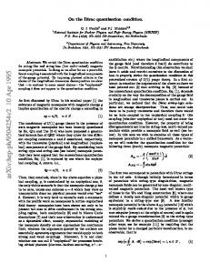
Finally, for the AN S potential we choose the following closed loop Γ (Fig. 2): start at (r, θ, φ) = (R, 0, 0) then go to (R, π, 0) along the θˆ direction (Γ1 ), then to (R, π, 2π) along φˆ (Γ2 above), then to (R, 0, 2π) along −θˆ (Γ3 ), and ˆ back to (R, 0, 0) (Γ4 ). The finally clockwise (along −φ) only nonvanishing contribution comes from Γ3 and equals Rπ 2πeg 0 sin θdθ = 4πeg and we arrive again at the Dirac quantization condition, Eq. (1). We note that the loop Γ constructed in this way, has several nice features. For single-valued potentials it reduces to Γ2 + Γ4 , which depending on where one has a singularity reduces to just Γ2 or Γ4 . For multi-valued potentials it picks up contributions through Γ1 + Γ3 . Let us now introduce the “generalized” covariant derivative used in Ref. [2]
z Γ4
x
y Γ2
Dµ = ∂µ − ieAµ − i˜ eA˜µ .
FIG. 1. The Γ2 and Γ4 contours (see text).
Here the gauge field Aµ is decomposed into transverse, Aµ = Tµν Aν , and longitudinal, A˜µ = Lµν Aν , components, coupled to charges e and e˜, respectively; we employ the projectors Lµν = ∂µ ∂ν /∂ 2 and Tµν = gµν − Lµν . The longitudinal components do not enter the field strength tensor Fµν and are unphysical. This theory is invariant under local U (1) transformations
For the A+ potential we choose a loop Γ4 in the −φˆ direction (clockwise) with r fixed and θ → 0 (Fig. 1) and obtain 4πeg = 2πn, which is the Dirac quantization condition, Eq. (1). Similarly, for A− we use a (counterclockwise) loop with θ → π (labeled Γ2 in Fig. 1) and obtain the same condition. The nontrivial content of this constraint is that the loop has been chosen so as to encircle the singular string: thus, Stokes theorem (which would state that the flux is zero since the encompassing area is zero) is not applicable. Had we chosen loop Γ2 for the potential A+ , the phase factor would be trivially unity, and no quantization condition could (or should) be obtained from this (poor) choice of integration contour. This is somehow an obvious statement but it will be useful later on in our discussion.
eAµ (x) + e˜A˜µ (x) → eAµ (x) + e˜A˜µ (x) − ∂µ Ω(x) . (6) By applying the projectors Lµν , Tµν on both sides of (6) one obtains 1 1 1 Aµ (x) → Aµ (x) − ∂µ Ω(x) + ∂µ 2 ∂ 2 Ω(x) e e ∂ 1 1 A˜µ (x) → A˜µ (x) − ∂µ 2 ∂ 2 Ω(x) . e˜ ∂
(7)
Thus, in the static case, as noticed in [2], the transverse components are left invariant and only the longitudinal ones change:
z
Γ3
(5)
A(r) → A(r)
Γ4
˜ → A(r) ˜ − 1 ∇Ω(r) , A(r) e˜
(8)
However, as pointed out in [5] this statement is ambiguous when the potential A is divergenceless, for then ∂ −2 Aµ cannot be defined. In fact, this is the case for all string–type potentials, since [3,5] Z (9) ∇ · A = 0, with A(r) = − du × B(r − u) .
x
Γ
y Γ1
1 ∇( 4πx Here B(x) = −g∇ ) and the Dirac string lies along a generic single–valued semi–infinite path Γ. But if the potential is divergenceless we can as well take the longitudinal part to be zero. Moreover, if we consider a (static) transformation ΩΓ,Γ′ that moves the Dirac string to lie along a different path Γ′ the above property guarantees
Γ2
FIG. 2. The Γ = Γ1 + Γ2 + Γ3 + Γ4 contour (see text).
2
that ∂ 2 ΩΓ,Γ′ = 0 and that under this gauge transformation the longitudinal component remains the same (trivially, since it is zero) while the transverse changes 1 A(r) → A(r) − ∇Ω(r) e ˜ → A(r) ˜ =0 . A(r)
• criterion (A): the flux through any closed loop shrunk to zero should be unobservable, that is I n I o e A · dl + e˜ A˜ · dl = 2πn, n ∈ Z , (15) Γ
where, as before, Γ is a closed loop surrounding a minimal surface with zero area.
(10)
This equation should be contrasted with Eq. (8). In order to be more specific let us discuss the longitudinal– transverse decomposition for the potentials in Eq. (3). He, Qiu and Tze offer the following decomposition into transverse and longitudinal components: (I)
A∓ = −
g cos θ ˆ ˜(I) g 1 ˆ φ, A∓ = ± φ. r sin θ r sin θ
We wish to emphasize that a finite contribution to the left hand side of Eq. (15) for “zero area” loops Γ can arise either because the potential is singular inside Γ or because there is no singularity but the potential is multi– valued around Γ. Thus, we impose two more criteria:
(11)
• criterion (B): we should not expect to obtain a constraint in the form of a quantization condition for loops inside which the potential is both smooth and single–valued.
Thus, the transverse piece is the same for the two strings and the gauge transformation that maps one string solution to the other is of the type (8) with Ω(r) = 2˜ egφ. However, as we said above, ∇2 Ω = 0 and thus we could as well have the decomposition (II)
A∓ = −
g cos θ ∓ 1 ˆ ˜(II) φ, A∓ = 0 . r sin θ
This criterion should be imposed because in the region where the potential is smooth and single–valued it is irrelevant whether it arises from a monopole string (which we want to make unobservable) or from a semi–infinite solenoid (which is put there by hand and is certainly observable). Any condition in this region would therefore constraing the possible values that the flux through the solenoid can take which is unphysical.
(12)
Notice that the gauge transformation that connects the two strings is now of the type (10) with Ω(r) = 2egφ which is the same as above but with the physical coupling, e, appearing instead of the unphysical one, e˜. What about the string–less potential AN S ? In this case we cannot take it to be purely transverse, since ∇·
sin θφ ˆ cos θ θ = 2 2 φ 6= 0 . r r
• criterion (C): When we decompose the string– less potential AN S into longitudinal and transverse parts we should be careful to avoid —if possible— introducing singularities because then we undo the very motivation for introducing such potentials, namely, that they are non–singular!
(13)
It is straightforward to check that all of the following are legitimate longitudinal–transverse decompositions for AN S :
It is easy to show that this latter criterion (C) can be locally (that is, for a subset of R3 ) satisfied: just add enough ∇φ = (1/r sin θ)φˆ terms so as to compensate for the singularity. For example, a singularity of the type (cos θ/r sin θ)φˆ which extends over the whole z axis can, ∇φ, be reduced to the half z axis. That by adding ±∇ means that we introduce a decomposition that is different in various space regions (` a la Wu and Yang), but the potential is multivalued anyway so that’s not a problem. In Table 1 we show the results for the Γ4 loop. We have made the choice AN S = A− for loop Γ4 , so as to keep the decomposition non–singular, in accordance with criterion (C).
g cos θ ˆ ˜(I) g cos θ ˆ g φ, AN S = φ − sin θφθˆ (14) r sin θ r sin θ r g cos θ ± 1 ˆ g g cos θ ± 1 ˆ ˜(II) φ, AN S = φ − sin θφθˆ . =− r sin θ r sin θ r (I)
AN S = − (II)
AN S
As before, decomposition (I) is the one used by He, Qiu and Tze [3]. In the decompositions (II+,II-) we have used our experience from the string–type potentials above to move ∇ φ = (1/r sin θ)φˆ pieces between the longitudinal and transverse parts since these terms can be equally well considered to be either longitudinal or transverse.1 In the next step, we are going to calculate the flux through the various loops that we have employed before, separating the flux coming from the longitudinal and the transverse parts. In order to discuss the results we will consider three criteria, starting with the one in (4) for this generalized version of QED:
Table 1: the r=fixed, θ → 0 loop Γ4
they have both zero curl and zero divergence
3
decomposition (I) decomposition (II) H H H H e Γ4 A · dl e˜ Γ4A˜ · dl e Γ4 A · dl e˜ Γ4A˜ · dl +2πeg
+2π˜ eg
+4πeg
0
A−
+2πeg
−2π˜ eg
0
0
AN S
+2πeg
−2π˜ eg
0
0
A+
1
Γ
Criterion (A) then implies the following constraints for the loop Γ4 and decomposition (I) for the three potentials (n ∈ Z throughout): n = g = 0, if e˜ arbitrary A+ : g(e + e˜) = n ⇒ (16) eg = n/2, if e˜ = e n = g = 0, if e˜ arbitrary A− : g(e − e˜) = n ⇒ no constraint, if e˜ = e n = g = 0, if e˜ arbitrary AN S : g(e − e˜) = n ⇒ no constraint, if e˜ = e ,
also for ordinary QED (e = e˜) one did not obtain such a condition from these loops. So let’s discuss the results for the loop Γ (Fig. 2). We have to add the contributions of Tables 1 and 2 and also add the contribution of the θˆ part of AN S to Γ3 (the contribution to Γ1 vanishes because φ = 0). The results are presented in Table 3. One sees that (a) the only quantization condition that can be obtained in this case is the conventional one eg = n/2, independent of the transverse–longitudinal decomposition one uses and (b) that the longitudinal terms lead to no constraint whatsoever. This is a direct consequence of the fact that the piece ∇φ does not contribute to the flux through the loop Γ in Fig. 2. Therefore, irrespective of the decomposition of the potential, the condition obtained from this loop is the ordinary quantization condition in Eq. (2).
while for the same loop Γ4 decomposition (II) implies A+ : ge = n/2 A− : no constraint AN S : no constraint .
(17)
Table 3: the loop Γ = Γ1 + Γ2 + Γ3 + Γ4
A number of observations can be made here:
2. Decomposition (I) implies individual quantization conditions for e− e˜ and e+ e˜. If we treat e˜ as independent of e and subtract these constraints we get Eq. (2) used in [2,3] to prove that QED is inconsistent with monopoles. However, we view this result as unphysical since for e˜ arbitrary decomposition (I) violates both (B) and (C) criteria. In particular it violates (B) by leading to a constraint (the second of Eqs. (16) above) coming from a potential, A− , which is smooth and single–valued in the area of the loop Γ4 . It also violates (C) by introducing singularities in the vicinity of loop Γ4 for the string–less potential AN S .
0
0
A−
+2πeg
+2π˜ eg
+4πeg
0
AN S
+2πeg
−2π˜ eg
0
0
0
A−
+4πeg
0
+4πeg
0
AN S
+4πeg
0
+4πeg
0
• No constraint on e˜ is imposed. Thus, even by treating the longitudinal coupling e˜ as arbitrary (despite the questions this raises for virtual photons) we have shown that quantum electrodynamics is consistent with magnetic monopoles.
decomposition (I) decomposition (II) H H H H ˜ e Γ2 A · dl e˜ Γ2A · dl e Γ2 A · dl e˜ Γ2A˜ · dl −2π˜ eg
+4πeg
• The only quantization condition that can be obtained is the conventional one, Eq. (1).
Table 2: the r=fixed, θ → π loop Γ2
+2πeg
0
We summarize: the fact that criterion (A) is applicable to any closed loop allow us to recover the conventional quantization condition ge = n/2 not only for string–type potentials where their divergenceless makes this result quite obvious but also when considering the string–less potential AN S which is not purely transverse. This result stems from the decomposition–independent Γ contour integrations in Table 3. Moreover, by imposing some physical criteria (B) and (C) for choosing a physical longitudinal–transverse decomposition we have shown that the freedom to move ∇ φ parts between longitudinal and transverse pieces amounts to the following:
Analogous remarks can be made for the A+ potential in the case of the Γ2 loop (see Table 2). In this case we have chosen AN S = A+ , in accordance with criterion (C).
A+
+4πeg
A+
1. Decomposition (II) meets all criteria (A), (B) and (C). Moreover, the only constraint it leads to is the conventional quantization condition ge = n/2.
decomposition (I) decomposition (II) H H H H e Γ A · dl e˜ ΓA˜ · dl e Γ A · dl e˜ ΓA˜ · dl
Acknowledgements: This work is supported in part by the Foundation for Fundamental Research on Matter (FOM) and the National organization for Scientific Research (NWO) as well as the Human Capital and Mobility Fellowship ERBCHBICT941430.
Notice that in our decomposition (II) so far these loops do not lead to a quantization condition stemming from the string–less, but multi-valued potential AN S . However, 4
[1] P.A.M. Dirac, Proc. Poy. Soc. (London) Ser. A, 133, 60 (1931). [2] H.-J. He, Z. Qiu and C.-H. Tze, Z. Phys. C 65, 175 (1994). [3] H.-J. He, Z. Qiu and C.-He, Virginia Polytechnic Institute preprint VPI-HEP-93-14 (1993). [4] H.-J. He and C.-H. Tze, Addendum to “Inconsistency of QED in the presence of Dirac Monopoles”, Z. Physik C (in press). [5] G.I. Poulis and P.J. Mulders, NIKHEF preprint NIKHEF-94-P11, Z. Physik C (in press). [6] T. Banks, R. Myerson and J. Kogut, Nucl. Phys. B 129 493 (1977); A.M. Polyakov in “Gauge Fields and Strings”, Harwood Academic Publishers, Chur, Switzerland (1987). [7] T.A. DeGrand and D. Toussaint, Phys. Rev. D 22, 2478 (1980), H. D. Trottier and R. M. Woloshyn, Phys. Rev. D 48, 4450 (1993). [8] T.T. Wu and C.N. Yang, Phys. Rev. Lett. 13, 380 (1964). [9] Sidney Coleman, Appendix 5 in “Classical lumps and their quantum descendants”, page 260, Aspects of Symmetry, Cambridge University Press (1988). [10] H.A. Cohen, Progr. Theor. Phys. Vol 50, No. 2, (1973). [11] T.-P. Cheng and L.-F. Li in “Gauge Theory of Elementary Particle Physics”, Oxford University Press (1984).
5