Eötvös Loránd University, Institute of Mathematics ... From mathematical point of ..... A., Plemmons, R.J.: Nonnegative matrices in the mathematical sciences.
On the Discretization Time-Step in the Finite Element Theta-Method of the Discrete Heat Equation Tam´as Szab´o E¨ otv¨ os Lor´ and University, Institute of Mathematics 1117 Budapest, P´ azm´ any P. S. 1/c, Hungary
Abstract. In this paper the numerical solution of the one dimensional heat conduction equation is investigated, by applying Dirichlet boundary condition at the left hand side and Neumann boundary condition was applied at the right hand side. To the discretization in space, we apply the linear finite element method and for the time discretization the wellknown theta-method. The aim of the work is to derive an adequate numerical solution for the homogenous initial condition by this approach. We theoretically analyze the possible choice of the time-discretization step-size and establish the interval where the discrete model is reliable to the original physical phenomenon. As the discrete model, we arrive at the task of the one-step iterative method. We point out that there is a need to obtain both lower and upper bounds of the time-step size to preserve the qualitative properties of the real physical solution. The main results of the work is to determine the interval for the time-step size to be used in this special finite element method and analyze the main qualitative characterstics of the model.
1
Preliminaries
Minimum time step sizes for different diffusion problems have been analyzed by many researchers [7]. Thomas and Zhou [4] have constructed an approach to develop the minimum time step size, that can be used in the finite element method of diffusion problems. However, these approach is rigorous. We point out its imperfections and extend the analysis to the theta method as well, and develop an upper limit for the maximum time step size. In this paper, for the analysis of the one-dimensional classical diffusion problem, the heat conduction equation is considered. Heat conduction or, in other terminology, the thermal conduction is the self-generated transfer of thermal energy through the space, from a place of higher temperature to a place of lower temperature, and thus is at work to even out the temperature gradients. From mathematical point of view this equation is the prototypical parabolic partial differential equation. S. Margenov, L.G. Vulkov, and J. Wa´ sniewski (Eds.): NAA 2008, LNCS 5434, pp. 564–571, 2009. c Springer-Verlag Berlin Heidelberg 2009 �
On the Discretization Time-Step in the Finite Element Theta-Method
565
The general form of this equation is ∂ 2T ∂T = k 2 , x ∈ (0, 1], t > 0, ∂t ∂x ∂T (1, t) = 0, t ≥ 0, T (0, t) = τ ; ∂x T (x, 0) = u0 (x), x ∈ (0, 1], c
(1)
where c represents the specific heat capacity, that is the measure of the thermal energy required to increase the temperature of a matter by a certain temperature level, T is the temperature of the analyzed domain, t and x denotes the time and space variables, respectively, k is the coefficient of the thermal conductivity, that is the property of a material that indicates its ability to conduct thermal energy. Moreover, τ is the temperature at x = 0, a non-negative real number. The lefthand side of this equation expresses the rate of the temperature change at a point in space over time and the right-hand side indicates the spatial thermal conduction in direction x. During the analysis of the problem the space was divided into n − 1 elements. The heat capacity and the coefficient of thermal conductivity are assumed to be constants. The boundary conditions are so-called mixed boundary conditions. The physical meaning of this type of boundary condition is that, at the end of the body the heat flux is zero, in other words the thermal energy can not leave the system. The weak form of the problem (1) is �
1
c 0
∂T ∂T v(x)dx + kv(0) (0, t) + ∂t ∂x
�
1
k 0
∂T dv dx = 0 ∂x dx
(2)
for all v ∈ H01 (0, 1), where H01 (0, 1) denotes the sub-space of Sobolev space H 1 (0, 1) with v(0) = 0. Hence, we seek such a function T (x, t), which belongs to H 1 (0, 1) for all fixed t, morover, there exists ∂T ∂t , and it satisfies (2) for all v ∈ H01 (0, 1). We seek the spatially discretized temperature Td in the form: Td (x, t) =
n �
φi (t)Ni (x),
(3)
i=0
where Ni (x) are given shape functions, (Fig. 1) and φi are unknown, and n is the ordinal number of nodes. The unknown temperature index starts from 1, because, due to the boundary condition at the first node the temperature is known, namely, φ0 (t) = τ . Substituting (3) into (2), we get the weak semidiscretized equation n � i=0
�
φi (t)
�
1
cNi (x)Nj (x)dx+ 0
+
n � i=0
� φi (t) 0
1
�
�
kNi (x)Nj (x)dx = 0, j = 1, 2 . . . n.
(4)
566
T. Szab´ o
Fig. 1. Linear shape functions
Let K, M ∈ R(n+1)×n denote the so-called mass and stiffness matrices, respectively, defined by: � 1 � � kNi (x)Nj (x)dx, (5) (K)ij = 0
�
1
(M )ij =
cNi (x)Nj (x)dx.
(6)
0
Then (4) can be expressed as: �
M Φ + K Φ = 0,
(7)
where Φ ∈ Rn+1 is a vector function with the components φi . For the time discretization of the system of ODE (7) we apply the well-known theta-method, which results in the equation M
� � Φm+1 − Φm + K ΘΦm+1 + (1 − Θ)Φm = 0. Δt
(8)
Clearly, this is a system of linear algebraic equations w.r.t. the unknown vector Φm+1 being the approximation of the temperature at the new time-level. Here the parameter Θ is related to the applied numerical method and it is an arbitrary parameter on the interval [0, 1]. It is worth to emphasize that for Θ = 0.5 the method yields the Crank-Nicolson implicit method which has higher accuracy for the time discretization [6]. In order to preserve the qualitative characteristics of the solution, the connections between the equations and the real problem must be analyzed. To obtain a lower bound for the time-step size, equation (6)-(8) should be analyzed. As it is well known, the temperature (in Kelvin) is a non-negative function in physics. In this article the following sufficient condition will be shown for the time-step size of the finite element theta-method to retain the physical characteristics of the solution: h2 c h2 c < Δt ≤ , (9) 6Θk 3(1 − Θ)k where h is the length of the spatial approximation. This sufficient condition is well known for problems with pure Dirichlet boundary conditions but not for
On the Discretization Time-Step in the Finite Element Theta-Method
567
the problems with mixed boundary conditions (Newton and Dirichlet), see e.g., [5] [3].
2
Analysis of FEM Equation
After performing the integral in (5) and (6) for the linear shape functions, the mass and the stiffness matrices have the following form ⎤ ⎤ ⎡ ⎡ −1 2 −1 . . . 0 1 4 1 ... 0 . ⎥ .⎥ . . 1⎢ h⎢ ⎢ . . . . . . . . . . .. ⎥ ⎢. .. .. .. .⎥ (10) K=k ⎢ . ⎥ , M = c ⎢. . . . .⎥ h ⎣ 0 . . . −1 2 −1⎦ 6 ⎣0 . . . 1 4 1⎦ 0 . . . 0 −1 1 0 ... 0 1 2 respectively. Using (10), the system (8) can be rewritten as:
where
m m aΦm+1 + bΦm+1 + aΦm+1 + eΦm 0 + f Φ1 + eΦ2 = 0 0 1 2
(2.2(1))
aΦm+1 1
=0 ...
(2.2(2))
m+1 m+1 m m aΦm+1 + eΦm n−2 + f Φn−1 + eΦn = 0 n−2 + bΦn−1 + aΦn b m+1 f m Φ =0 + eΦm aΦm+1 n−1 + n−1 + Φn 2 2 n
(2.2(n-1))
+
bΦm+1 2
+
aΦm+1 3
+
eΦm 1
+
f Φm 2
+
eΦm 3
hc hc Θk Θk − , b=2 + , 6Δt h 3Δt h
(1 − Θ) k (1 − Θ) k hc hc − , f =2 − . e=− 6Δt h h 3Δt a=
(2.2(n))
(11) (12)
Clearly b > 0. First we analyze the case when homogenous initial condition is given, i.e., u0 (x) = 0. Then Φ0i = 0, (i = 1, 2, ..., n). Since τ > 0, therefore, it is worth to emphasizing that, if τ is greater than zero, there is a discontinuity in the initial conditions at the point (0, 0). We investigate the condition under which the first iteration, denoted by Φ=Φ1 , results in non-negative approximation. The equations (2.2(1))-(2.2(n)) can be rewritten as aΦ0 + bΦ1 + aΦ2 = 0
(2.5(1))
aΦ1 + bΦ2 + aΦ3 = 0 ...
(2.5(2))
aΦn−2 + bΦn−1 + aΦn = 0 b aΦn−1 + Φn = 0 2
(2.5(n-1)) (2.5(n))
568
T. Szab´ o
When a = 0, then the solution of this equation system is equal to zero. This means that the numerical scheme doesn’t change the initial state which contradicts to the physical process. Therefore, in the sequel we assume that a �= 0. We seek the solution in the following form Φi = Zi Φ0 , i = 0, 1, ..., n.
(13)
Obviously, Z0 = 1. Using (2.5(n)), Zn can be expressed as Zn = − where
2a Zn−1 = Xn−1 Zn−1 , b
2a . b can be expressed from (2.5(n-1)). applying (7): Xn−1 = −
In the next step, Zn−1
Zn−1 = −
1 Zn−2 = Xn−2 Zn−2 , b + Xn−1 a
where Xn−2 = −
1
b + Xn−1 a For the i-th equation the following relation holds: Zi = −
.
1 Zi−1 = Xi−1 Zi−1 , i = 1, 2, ..., n − 1, b + Xi a
(14)
(15)
(16)
(17)
(18)
where
1 , i = n − 1, n − 2, ..., 1. b + Xi a Hence we obtained the following statement. Xi−1 = −
(19)
Theorem 1. The solution of the system of linear algebraic equations (2.5) can be defined by the following algorithm. 1. 2. 3. 4.
We put Z0 = 1; We define Xn−1 , Xn−2 , ..., X0 by the formulas (8) and (12), respectively; We define Z1 , Z2 , ..., Zn by the formulas (7) and (11), respectively; By the formula (6) we define the values of Φi .
The relation Φi ≥ 0, holds only under the condition Zi ≥ 0. From (11) we can see that it is equivalent to the non-negativity of Xi for all i = 0, 1, ..., n − 1. Therefore, based on (12), we have the condition a < 0 since b > 0. For the analysis of the non-negativity of the numerical solution, produced by the above algorithm, we will use the following trivial statement.
On the Discretization Time-Step in the Finite Element Theta-Method
569
Lemma 2. Assume that c > 2 and let us define the recursion as follows ai+1 = 1 . When a1 ∈ (0, 1) then ai ∈ (0, 1) for any indices. c − ai This lemma implies that under the condition −b/a > 2 each element Xi is non-negative, because the condition Xn−1 = −2a/b ∈ (0, 1) is automatically satisfied. The non-negativity of a yields the condtion a=
Θk hc − < 0. 6Δt h
(20)
that is, we got the condition h2 c < Δt. 6Θk Hence, the following statement is proven.
(21)
Theorem 3. Let us assume that the condition (14) holds. Then for the problem (1) with homogenous initial condition the linear finite element method results in a non-negative solution on the first time level. Naturally we are interested in the non-negativity preservation property not only at the first time level but on each ones. This means that rewritting the system (2.2(1))-(2.2(n)) in the matrix-vector form AΦm+1 = f m ,
(22)
we must garantee the inverse-positivity of the matrix A and the non-negativity of right hand side f m . Since under the condition (14) the realtions b > 2|a| and a < 0 are valid, therefore, A is a strictly diagonally dominant M-matrix and hence its inverse is non-negative matrix [2]. The second condition can be guaranteed for arbitrary Φm if and only if e and f are non-positives. Obviously the condition e < 0 is always true, therefore the only condition, which should be satisfied, is the requirement f ≤ 0, i.e., Δt ≤
h2 c . 3(1 − Θ)k
(23)
Theorem 4. Let us assume that the time discretization parameter Δt satisfies the condition (9). Then for the problem (1) with arbitrary non-negative initial condition the linear finite element method results in a non-negative solution on any time level.
3
Numerical Experiments
In the numerical experiments for the boundary condition at left hand side of the space domain we put the value τ = 273. For the numerical experiments, a
570
T. Szab´ o
400 350
Temperature [K]
400
300
300
250
200
200 150
100
100 0 20
10 20
15
50
30
10 5
40 50
Node
Timestep
Fig. 2. The solution applying to high time step
250
200
Temperature [K]
400 300
150
200 100 100 0 20
10
50
20
15
30
10 5
40 50
Node
Timestep
Fig. 3. The solution applying time step from the interval (16)
special type of Gauss elimination was used for the inversion of the sparse tridiagonal matrices [1]. The following figures are in three dimensions, the first dimension is the length of a node, the second one is the temperature at the nodes, and the third one is the estimated time since the model start. First, we apply relatively high time-step, that causes the positivity of F . In (Fig. 2) one can see the numerical method is quite unstable, hence there is an oscillation with decreasing tendency in the results. When we apply smaller time steps than, in (16), close to the first node, there will be small negative peaks, that is an unrealisctic solution, since the absolute temperature should be non-negative.
On the Discretization Time-Step in the Finite Element Theta-Method
571
For the sake of completeness In Fig. 3 we applied the time-step size from the interval (16), and it can be seen that the oscillation disappears and we have got more stable numerical method. It is easy to see, that, by use of appropriate time steps, the solution becomes much smoother than in the Fig. 2.
4
Conclusions and Further Works
In this article the sufficient condition was given for the time-step size of the finite element theta-method to preserve the physical characteristics of the solution. For the homogenous initial condition we have shown that there exists only the lower bound for the time-step size of the finite element theta method., in order to preserve the non-negativity at the first time level. When we were interested in the non-negativity preservation property not only at the first time level but on the whole discretized time domain, then, by applying arbitrary initial condition, we shown the existence the bounds from both directions, i.e., there are upper and lower bounds for the time-step, as well. Finally, we note that all results can be extended to the higher dimensional parabolic heat equation. In this case in (1.8) the mass (M) and stiffnes (K) matrices are block tridiagonal matrices, in the equations (2.2(1))-(2.2(n)) the corresponding coefficients are matrices and the unkown are vectros in each row. Therefore the conditions (2.14) and (2.16) can computed analogically. Detailed analysis of this problem will be down in the future.
References 1. Samarskiy, A.A.: Theory of different schemes. Moscow, Nauka (1977) (in Russian) 2. Berman, A., Plemmons, R.J.: Nonnegative matrices in the mathematical sciences. Computer Science and Applied Mathematics, 316 p. Academic Press (Harcourt Brace Jovanovich, Publishers), New York-London (1979) 3. Farkas, H., Farag´ o, I., Simon, P.: Qualitative properties of conductive heat transfer. In: Sienuitycz, S., De Voseds, A. (eds.) Thermodynamics of Energy Conversion and Transport, pp. 199–239 (2000) 4. Thomas, H.R., Zhou, Z.: An analysis of factors that govern the minimum time step size to be used in finite element analysis of diffusion problems. Commun. Numer. Meth. Engng. 14, 809–819 (1998) 5. Farago, I.: Non-negativity of the difference schemes. Pour Math. Appl. 6, 147–159 (1996) 6. Crank, J., Nicolson, P.: A practical method for numerical evaluation of solutions of partial differential equations of the heat conduction type. Proceedings of the Cambridge Philosophical Society 43, 50–64 (1947) 7. Murti, V., Valliappan, S., Khalili-Naghadeh, N.: Time step constraints in finite element analysis of the Poisson type equation. Comput. Struct. 31, 269–273 (1989)