M/D/1, M/M/â, and M/D/â queues, respectively. Keywords: Capacitated/uncapacitated supplier, Make-to-stock queue, Advance demand information, Order ...
Liberopoulos-Koukoumialos, 95-114
On the Effect of Variability and Uncertainty in Advance Demand Information on the Performance of a Make-to-Stock Supplier George Liberopoulos Department of Mechanical and Industrial Engineering, University of Thessaly, Greece Stelios Koukoumialos Department of Financial and Management Engineering, University of the Aegean, Greece
Abstract Our aim in this paper is to investigate how variability and uncertainty in advance demand information (ADI) affects the performance of a make-to-stock supplier. To this end, we develop a model of a supplier who receives orders for one item at a time from customers that may belong to one of two classes. Each customer in the first class requests immediate delivery, and hence provides no ADI at all. Each customer in the second class makes a cancelable reservation in advance of his requested due date, and hence provides uncertain ADI. We assume that the supplier uses an order base stock replenishment policy with a release lead time. According to this policy, each customer order triggers the potential placement of a replenishment order by the supplier at a time that is determined by offsetting the demand due date by a fixed planned supply lead time. The replenishment order is actually placed only if there have been fewer cancellations that replenishment orders in the past; otherwise, it is skipped. We investigate via simulation the impact of important ADI related parameters on the optimal decision variables and performance of the replenishment policy, for four different variations of the model. In each variation, the replenishment (or supply) process is represented by a different queueing system. The systems that we consider are the M/M/1, M/D/1, M/M/∞, and M/D/∞ queues, respectively. Keywords: Capacitated/uncapacitated supplier, Make-to-stock queue, Advance demand information, Order base stock policy JEL Classification: M11
Introduction Production and operations management researchers and practitioners agree that obtaining and distributing demand information to all the partners of a supply chain is essential for improving the coordination and ultimately the performance of the supply chain. The benefits of sharing demand information are further amplified when this information is obtained ahead of time. From a supplier’s side, one of the main advantages of having access to advance demand information (ADI) is that such information can be used as a tradeoff for finished goods (FG) inventory and can thus lead to reduced inventory costs. One way that a supplier can obtain ADI is by inciting his customers to place their orders ahead of time. This can be accomplished by offering incentives such as price discounts or service priority to customers who order in advance. In many real situations, however, not all customers who are given the opportunity to order in advance will do so, and of those who will, some may subsequently change or cancel their orders; therefore, in practice, ADI is usually both variable and uncertain. Yet, with a few
MIBES Transactions, Vol 2, Issue 1, Autumn 2008
95
Liberopoulos-Koukoumialos, 95-114
exceptions, most of the literature on ADI concerns models in which ADI is assumed to be known with certainty (and in many cases to be even constant), perhaps because the literature on ADI is still in its early stages and such models are naturally the first to be developed and analyzed. Some of that literature is reviewed in the next section. Consequently, the self-evident managerial interest in assessing the impact of variability and uncertainty in the amount of ADI has not been satisfactorily addressed in the literature. The nature of the beneficial tradeoff between FG inventory and ADI, even when ADI is constant, is in general very difficult to assess analytically, particularly when the supplier is a capacitated production/inventory system, because production capacity affects this tradeoff in a non-trivial way. When ADI is variable and uncertain, the difficulty in obtaining analytical results seems insurmountable. Given the managerial interest in assessing the impact of variability and uncertainty in the amount of ADI on the supplier’s performance, but also the intricacy in carrying out this assessment analytically, in this paper we investigate this impact via simulation. Our hope is that the results of our investigation may shed some light into the nature of the tradeoff between FG inventory and ADI, and may provide some supporting evidence and intuition to more courageous researchers who set off to find analytical answers. To carry out our investigation, first we develop a model of a make-to-stock supplier who has access to variable and uncertain ADI. The supplier receives orders for one item at a time from customers that may belong to one of two classes. Each customer in the first class requests immediate delivery (rush job), and hence provides no ADI at all. Each customer in the second class makes a cancelable reservation a fixed demand lead time in advance of his requested due date, and hence provides uncertain ADI. Once he makes a reservation, he must subsequently confirm or cancel it a fixed confirmation lead time before this due date. We assume that the supplier uses a modified order base stock replenishment policy with a release lead time. According to this policy, each customer order triggers the decision by the supplier to place or not a replenishment order. The time of this decision is determined by offsetting the demand due date by a fixed planned supply lead time. When this decision time comes, the supplier decides to place the order only if there have been fewer cancellations than replenishment orders in the past; otherwise, he skips the order. The parameters of the modified policy are the order base stock level and the planned supply lead time. To investigate the impact of variability and uncertainty of ADI on the performance of the supplier, we study the impact of the ADI related parameters on the optimal decision variables and performance of the modified order base stock policy with a release lead time, for four variations of our model. In each variation, the replenishment (supply) process is represented by a different queueing system. The four systems that we consider are the M/M/1, M/D/1, M/M/∞, and M/D/∞ queueing systems, respectively. The first two systems are single-server queues and hence represent capacitated suppliers, whereas the latter two systems are infinite-server queues and hence represent uncapacitated suppliers. In our investigation we seek to address the following questions for we which we have no a priori intuition. The first set of questions is related to the impact of the demand lead time (denoted by T) of class-2 customers on the optimal decision variables and performance of the supplier’s replenishment policy. One of these variables is the order base stock level. The order base stock level can be viewed as
MIBES Transactions, Vol 2, Issue 1, Autumn 2008
96
Liberopoulos-Koukoumialos, 95-114
being made up of two components. The first component is aimed at ensuring adequate service to class-1 customers (rush jobs), while the second component is aimed at ensuring adequate service to class-2 customers. Intuition and previous analysis for the case where the supplier has constant, reliable ADI, i.e., only class-2 customers (e.g., see Liberopoulos (2008) and reference therein), suggest that as T increases, the optimal order base stock level should decrease until it reaches a certain minimum level at certain critical value of T. If this turns out to be true in the more complex model examined in this paper, where there are two classes of customers, then what is this minimum order base stock level equal to, and what is the corresponding critical value of T? What happens if T is larger than the critical value? Does the component of the optimal order base stock level aimed at servicing class-1 customers decrease also, given that the rush orders from class-1 customers can be satisfied by FG inventory replenishments triggered by class-2 customer orders? How does the optimal planned supply lead time vary with T? Another set of questions is related to the impact of the rush job probability (denoted by p), the cancellation probability (denoted by q), and the confirmation lead time (denoted by ) on the optimal parameters and performance of the modified order base stock policy with a release lead time. Intuition suggests that as p decreases, i.e., as there are fewer rush jobs, the amount of ADI increases, and therefore the supplier’s optimal order base stock level and cost should decrease. At the same time, as p decreases, the overall percentage of cancelled reservations, (1 – p)q, increases. As a result, the number of superfluous replenishment orders, i.e., orders that are triggered by eventually cancelled reservations, also increases, raising FG inventory along the way. Intuition suggests that this increase in FG inventory should cause a further decrease in the supplier’s optimal order base stock level and resulting cost. To summarize, as p decreases, intuitively the supplier’s optimal order base stock level and cost tends to also decrease. Does the optimal planned supply lead time also decrease with p? What is the impact of q and on the optimal decision variables and performance of the modified order base stock policy with a release lead time? Is it as simple to guess as the impact of p? Intuition suggests that as q decreases, i.e., as there are fewer cancellations, or increases, i.e., the confirmation lead time becomes longer, the uncertainty of ADI decreases, and therefore the supplier’s optimal order base stock level and cost should decrease. At the same time, as q decreases or increases, the supplier places fewer superfluous replenishment orders, causing a reduction in FG inventory. Intuition suggests that this reduction in FG inventory should cause an increase in the supplier’s optimal order base stock level to keep the customer service from dropping. To summarize, as q decreases or increases, intuitively the supplier’s optimal order base stock level and cost tend to both decrease and increase. Which of the two effects predominates? Finally, how does capacity interfere with variability and uncertainty in ADI, and does a capacitated supplier, whose replenishment orders are typically pipelined, behave differently than an uncapacitated supplier, whose replenishment orders do not necessarily arrive in the order in which they were placed? The rest of this paper is organized as follows. In the following section, we review some of the literature on ADI, particularly that which is most closely related to our work. Next, we describe our model, and then we investigate via simulation the impact of important ADI related parameters
MIBES Transactions, Vol 2, Issue 1, Autumn 2008
97
Liberopoulos-Koukoumialos, 95-114
on the optimal replenishment policy decision variables and performance of our model, for the cases where the supply process is modeled as an M/M/1, M/D/1, M/M/∞, and M/D/∞ queue, respectively. Initially, we look at the simpler case where there are no cancellations, and then we examine the more complicated general case with cancellations. We conclude at the last section.
Literature review The literature on ADI is growing fast. Most of it concerns pure inventory systems, i.e., systems with no production capacity and hence queueing effects. One of the earliest and most influential works for systems with exogenous replenishment times is the work of Hariharan and Zipkin (1995). They study a model of a supplier who uses a continuous-review order-basestock replenishment policy to meet customer orders that arrive according to a Poisson process. Each customer order is for a single item to be delivered a fixed demand lead-time following the order. They consider three cases for modeling the demand and replenishment (i.e., supply) lead-times. In each case, they construct an equivalent conventional model, i.e., one with no demand lead-times, in which the replenishment lead-times are offset by the demand lead-times. This shows that the effect of a demand lead-time on overall system performance is the same as a corresponding reduction in the replenishment lead-time. Gallego and Özer (2001) consider a single-stage periodic-review inventory system with exogenous replenishments and variable but finite demand leadtimes. They show that for the zero set-up cost case, an order-base-stock policy is optimal if the replenishment time is greater than the maximum demand lead-time. Gallego and Özer (2003) and Özer (2003) extend this analysis to multi-echelon and distribution systems, respectively, and Wang and Toktay (2006) extend it to systems with flexible delivery. Finally, Özer and Wei (2004) prove the optimality of a state-dependent modified order-base-stock policy for an extension of the single-stage system in which the capacity is limited. Other works that show replenishment times are Mookerjee (1997), Chen (2003), Marklund (2006),
the benefits of ADI on systems with exogenous Bourland et al. (1996), Güllü (1997), Decroix and (2001), van Donselaar et al. (2001), Lu et al. and Tan et al. (2007).
For queue-type capacitated production/inventory systems, Buzacott and Shanthikumar (1993, 1994) present a detailed model of a single-stage maketo-stock manufacturer who uses a continuous-review order-base-stock replenishment policy to meet customer demands that arrive a fixed demand lead-time in advance of their due-dates. They analyze in detail the case where demands arrive according to a Poisson process and the manufacturing system consists of a single server with exponentially distributed processing time and FCFS service protocol; hence, the flow through the manufacturing system is identical to that through an M/M/1 queue. For this system, they show that the optimal demand lead-time and associated cost is a linearly decreasing function of the order-base-stock level. For the discrete-time version of the M/M/1 make-to-stock manufacturing system analyzed in Buzacott and Shanthikumar (1993, 1994), Karaesmen et al. (2002) evaluate analytically the performance of the optimal order-basestock policy. They then compare it to the performance of the overall optimal replenishment policy, which they evaluate numerically using dynamic programming. Their numerical results show that the optimal order-base-stock policy is quite effective.
MIBES Transactions, Vol 2, Issue 1, Autumn 2008
98
Liberopoulos-Koukoumialos, 95-114
Karaesmen et al. (2003) complement the work of Buzacott and Shanthikumar (1993, 1994) with some results on the influence of production lead-time variability on the tradeoff between the order-base-stock level and the demand lead-time. Along the way, they propose an approximation scheme for a generalization of the model studied by Buzacott and Shanthikumar (1993, 1994) in which the flow through the manufacturing system is identical to that through an M/G/1 queue. Karaesmen at al. (2004) assess the value of ADI for the model considered by Buzacott and Shanthikumar (1993, 1994) by assuming that the manufacturer pays a fixed or a demand lead-time-dependent price for obtaining ADI. They then evaluate the effects of processing capacity on the value of ADI. They repeat this assessment for a variation of the model in which customers accept deliveries earlier than their required due-dates. For this variation, they show that the effect of a demand lead-time on overall system performance is the same as a reduction in the backorder cost in an equivalent conventional system, i.e., one with no demand lead-times. Liberopoulos et al. (2003) propose an order-base-stock-type policy for a model of a make-to-stock supplier with two classes of customers: those who provide unreliable ADI in the form of cancelable reservations, and those who provide no ADI at all. They optimize this policy via simulation. Gayon et al. (2006) and Benjaafar et al. (2006) use Markov decision process analysis to characterize the structure of the optimal policy of a singlestage capacitated supply system with imperfect ADI, where customers either make cancelable reservations, as in the system introduced by Liberopoulos et al. (2003), or provide changeable due-dates, respectively. Liberopoulos et al. (2005) investigate via simulation the tradeoff between the optimal order-base-stock levels and kanbans (WIP-control limits) and the demand lead-time, in order-base-stock policies with/without WIP-limits, for a single- and a two-stage make-to-stock capacitated manufacturing system with ADI. Wijngaard (2004) considers a single-stage make-to-stock manufacturing system that either produces at a constant production rate R or not all. The goal is to meet customer orders with minimum average inventory and stockout costs; both cases of lost sales and order backlogging are considered. Customer orders arrive according to a Poisson process a fixed demand leadtime h in advance of their due-dates. The flow through the manufacturing system is therefore equivalent to that through an M/D/1 queue, except that production is continuous. The main result is that for high utilization rate and small demand lead-times the finished-goods inventory reduction due to the foreknowledge of ADI is equal to (1 – ) h R. Wijngaard and Karaesmen (2007) show that for the make-to-stock M/D/1-type queue considered in Wijngaard (2004), if the demand lead time is smaller than a certain threshold value, then an order base stock policy is optimal. For unit production rate, this threshold value is equal to the optimal base stock level for the case without ADI. Finally, Liberopoulos (2008) develops some analytical results on the tradeoff between FG inventory and ADI for a model of a single-stage, maketo-stock supplier who uses an order base stock replenishment policy to meet customer orders that arrive a fixed time in advance of their due dates. Model description We consider a model of a make-to-stock supplier who has access to variable and uncertain ADI. The supplier receives orders for one item at a time from
MIBES Transactions, Vol 2, Issue 1, Autumn 2008
99
Liberopoulos-Koukoumialos, 95-114
customers that arrive randomly according to a stationary Poisson process with mean arrival rate . Each arriving customer may belong to one of two classes, 1 and 2. Each customer in class 1 requests immediate delivery (rush job), i.e., his requested due date coincides with the arrival time of his order. Each customer in class 2 makes a cancelable reservation a fixed time, T, before his requested due date. We refer to T as the demand lead time. For both classes, if no items are available at the requested due date, the demand is backordered. If we let R denote the demand lead time of any customer, then 0, for class-1 customers, R = (1) T, for class-2 customers. Each arriving customer belongs to class 1 or 2 with a fixed probability p and 1 – p, respectively. We refer to p as the rush job probability. Once a class-2 customer makes a reservation, he must subsequently confirm or cancel this reservation a fixed time, , prior to his requested due date. We refer to as the confirmation lead time. Note that if > T, offsetting the demand due date by would yield a time instant that preceded the customer order arrival time. In this case, the customer would have to confirm or cancel his order before he even places it. Since this is impossible, we assume that in this case, the customer must confirm or cancel his reservation immediately upon arrival. Therefore, the time instant at which a class-2 customer confirms or cancels his reservation is (T – )+ (2) time units after his arrival, where x+ ≡ max(0, x). If a class-2 customer confirms his reservation, the remaining time until he claims his item at his requested due date is T – (T – )+ = min(T, ). (3) Each class-2 customer cancels or confirms his reservation with a fixed probability q and 1 – q, respectively. We refer to q as the cancellation probability. Given that customers arrive according to a Poisson process with mean arrival rate and that all class-1 customers and a fraction (1 – q) of class-2 customers consume FG items, the total demand for the consumption of items from FG inventory is Poisson with rate [p + (1 – p)(1 – q)]. (4) e = The reservation-confirmation mechanism described above can also be viewed as a surrogate for a forecasting system in which there are some confirmed orders in the short term and forecasts of orders in the longer term. The parameters that affect the variability and uncertainty of ADI are , T, p, q, and . There is no setup cost or setup time for placing a replenishment order and no limit on the number of orders that can be placed per unit time. The supplier uses a type of an order base stock replenishment policy which we call modified order base stock policy with a release lead time. To describe how this policy works, we must first explain how the conventional order base stock policy with a release lead time works. The conventional order base stock policy with a release lead time, which was first proposed by Karaesmen et al. (2002), works like the classical base stock policy, except that each replenishment order is triggered by a customer order instead of an actual demand, and the time of placing this order is offset from the due date by a fixed time L, just like in the time phasing step of the MPR procedure. We refer to L as the planned supply lead time. Moreover, the supplier starts with an initial level of items in FG inventory, S, as in the classical base stock policy. We refer to S as the order base stock level. The advantage of the conventional order base stock policy with a
MIBES Transactions, Vol 2, Issue 1, Autumn 2008
100
Liberopoulos-Koukoumialos, 95-114
release lead time is that it requires minimal information and is very simple to implement. Moreover, under some conditions, it has been shown to be effective or even optimal. In the modified order base stock replenishment policy with a release lead time that we propose in this paper, each customer order does not necessarily trigger the placement of a new replenishment order by the supplier. If it did, then in the long run more replenishment orders than actual customer demands would be placed – since some customer reservations are cancelled – leading to the accumulation of infinite FG inventory. The decision to place or not a replenishment order is offset from the due date by the planned supply lead time, L. We refer to this decision as place-orskip decision, for short. Once again, note that if the demand lead time T is smaller than L, then offsetting the demand due date by L would yield a time instant that preceded the customer order arrival time, which means that the supplier would have to make his place-or-skip decision before the customer order even arrives. Since this is unreasonable, we assume that in this case the supplier makes his place-or-skip decision immediately upon the arrival of the customer order. Therefore, the time instant of the supplier’s place-or-skip decision is for class-1 customers, 0, (R − L)+ = + (5) − ( T L ) , for class-2 customers, time units after the arrival of a customer order. The outcome of the supplier’s place-or-skip decision is determined as follows. At the time instant of the place-or-skip decision, the supplier compares the cumulative number of cancelled reservations against the cumulative number of replenishment orders that have been placed up to that instant. If there have been more cancelled reservations than replenishment orders, then the supplier simply skips placing a new replenishment order. If there have been fewer cancelled reservations than replenishment orders, then the supplier places a new replenishment order immediately. To keep track of the surplus of the cumulative number of canceled reservations over the cumulative number of replenishment order placements, the supplier uses a stack which we call cancelled reservations surplus stack (CRSS), whose level increases/decreases as follows. Whenever a customer cancels his reservation, the CRSS level is increased by one. Whenever the CRSS is not empty at a place-or-skip decision instant, the supplier skips a replenishment order and the CRSS level is decreased by one; otherwise he places an order and leaves the CRSS level unchanged. If the supplier’s decision is to place an order, he does so immediately and receives one item after W time units. We refer to W as the actual replenishment (or supply or flow) time. W is a random variable that depends on the supply process. A schematic representation of the model that we described above is shown in Figure 1, where big circles represent delays, small circles represent probabilistic routing, and squares represent decision points. To better understand how the modified order base stock policy with a release lead time works, a typical sequence of events is shown in Figure 2, for the case where L < < T. The policy that we described above is reasonable, because it guarantees that in the long run, the supplier places as many replenishment orders as there are confirmed demands. Moreover, we think that it should also be quite effective, because in his place-or-skip decision, the supplier uses the most recent information on cancelled reservations. An alternative, simpler policy would be, for example, for the supplier to simply decide to
MIBES Transactions, Vol 2, Issue 1, Autumn 2008
101
Liberopoulos-Koukoumialos, 95-114
place or skip a replenishment order with stationary probability 1 – q and q, respectively. Such a policy would also guarantee that in the long run the supplier places as many replenishment orders as there are confirmed demands; however, it would probably be less effective than the modified order base stock replenishment policy we described in the previous paragraphs, because it uses no feed-back information on cancelled reservations. If CRSS is not empty, do not place replenishment Delay before making a order. Decrease CRSS by place-or-skip decision one. (R – L)+ Customer orders Rush jobs p
1 – p
If CRSS is empty, place replenishment order immediately. Delay before confirming a reservation (T – )+
Reservations
Replenishment Time W
Delay before demanding an item min(T, )
1 – q
FG inventory
e
Items to customers
Backordered demands
q
Cancelled reservations. Increase CRSS by one.
Confirmed reservations CRSS
Figure 1: Model of a single-stage, make-to-stock supplier with variable, unreliable ADI, operating under a modified order base stock replenishment policy with a release lead time T L t1 −
− − − −
t2
t3
t4
t5
time
At t1, a class-1 customer order arrives. The class-1 customer immediately demands an item, and the supplier decides to place or skip a replenishment order based on the current CRSS level. If his decision is to place the order, then he places it immediately. At t2, a class-2 customer order arrives. At t3, the class-2 customer confirms or cancels his order. If he cancels his order, the CRSS level is increased by one. At t4, the supplier decides to place or skip a replenishment order based on the current CRSS level. If his decision is to place the order, then he places it immediately. At t5, the class-2 customer demands an item.
Figure 2: Typical sequence of events for the case where L
: In this case, every class-2 customer confirms or cancels his reservation immediately upon arrival. This model is equivalent to a model in which there are no cancellations and the supplier has two classes of customers, namely, rush jobs and customers who place orders T time units in advance of their requested due dates. In the equivalent model, class-1 customers arrive according to a Poisson process with rate p, and class-2 customers arrive according to a Poisson process with rate (1 – p)(1 – q). The supplier always places – i.e., never skips – a replenishment order immediately upon the arrival of a customer order. p = 0: In this case, the supplier has a single class of customers, namely, customers who make cancelable reservations T time units in advance of their requested due dates. Customer orders, i.e., reservations, arrive according to a Poisson process with rate , and the consumption of items from FG inventory occurs according to Poisson process with rate (1 – q). Here, there are two subcases to consider. The first is the subcase where > L or L > > T. In this case, the resulting model is equivalent to a model in which customers arrive according to a Poisson process with rate (1 – p), there are no cancellations, each customer places a firm order min(T, L) time units in advance of his requested due date, and each customer order immediately triggers the placement of a new replenishment order. The second subcase is one in which < L and < . In this case, the resulting model is equivalent to a model in which customer reservations arrive according to a Poisson process with rate , each customer must confirm/cancel his reservation min(T, L) – time units after he places it. If a customer confirms his reservation, the remaining time until he claims his item at his requested due date is . p = 1: In this case, the supplier has a single class of customers, namely, rush jobs, so there is no ADI. Customer orders, i.e., demands, arrive according to a Poisson process with rate . Parameters T, L, , and q are irrelevant. The supplier uses a classical base stock policy, namely, he always places a replenishment order immediately upon the arrival of a customer demand. This case is identical to the case where T = 0, except that the customer demand arrival rate is instead of e. q = 0: In this case, there are no cancellations. The supplier has two classes of customers, namely, rush jobs and customers who place orders T time units in advance of their requested due dates. Class-1 customers arrive according to a Poisson process with rate p, and class-2 customers arrive according to a Poisson process with rate (1 – p). Parameter is irrelevant. The supplier always places – i.e., never skips – a replenishment order (R – L)+ time units after the arrival of a customer order. This case is similar to the equivalent model in the case where >
MIBES Transactions, Vol 2, Issue 1, Autumn 2008
103
Liberopoulos-Koukoumialos, 95-114
T, except that in that model, the supplier always places a replenishment order immediately upon the arrival of a customer order. q = 1: In this case, all reservations are cancelled. This model is equivalent to a model in which the supplier has a single class of customers, namely, rush jobs, so there is no ADI. Customer orders, i.e., demands, arrive according to a Poisson process with rate p. Parameters T, L, and , are irrelevant. The supplier uses a classical base stock policy, namely, he always places a replenishment order immediately upon the arrival of a customer demand. This case is identical to the case where T = 0, except that the customer demand arrival rate is p instead of e. p = q = 0: In this case, there are no cancellations, and the supplier has a single class of customers, namely, customers who place their orders T time units in advance of their requested due dates. Customer orders arrive according to a Poisson processes with rate . This case represents the situation where the supplier has access to constant, reliable ADI (see Liberopoulos, 2007). Effect of variability and uncertainty in ADI on the supplier’s performance We consider a standard optimization problem whose objective is to find the values of S and L that minimize the long-run expected average cost of holding and backordering FG inventory, for given ADI related parameters , T, p, q, and , and inventory holding and backordering cost rates, h and b, respectively. Our goal is to investigate the impact of the ADI related parameters on the supplier’s optimal decision variables and performance. We carry out our investigation for four variations of the model that we developed in Section 0, where in each variation the supply process is represented by a different queueing system. The four systems that we consider are the M/M/1, M/D/1, M/M/∞, and M/D/∞ queues, respectively. The cost rates h and b are the same in all the variations and are set equal to 1 and 9, respectively. For each variation, we consider two different values for the customer arrival rate, namely = 0.8 and = 0.95. For each queueing system variation and for each value of , the service rate of the queueing system, denoted by , is set so that E[W] = 5 in order to have a common basis when comparing the results between different systems. Note that for the M/M/1 and M/D/1 queues, E[W] is equal to 1/ (1 – ) and 1/ + 2 /2(1 – ) , respectively (e.g., see Gross and Harris, 1998), whereas for the M/M/∞ and M/D/∞ queues, E[W] is simply equal to 1/ . To carry out our investigation, we proceed step by step. Initially, we look at the simpler case where there is no order canceling; hence ADI is variable but reliable. Then, we look at the more complicated general case where ADI is both variable and unreliable. Effect of variability First, we investigate the case where q = 0. As we mentioned in the previous section, when q = 0, there are no cancellations; hence ADI is variable but reliable. Parameter is irrelevant and the supplier always places a replenishment order (R – L)+ time units after the arrival of a customer order. A schematic representation of the resulting model is shown in Figure 3. Let L* denote the optimal planned supply lead time. Let S*(T) and C*(T) denote the optimal order base stock level and the corresponding minimum long-run expected average cost, when the planned supply lead time is L* and the demand lead time is T. As was mentioned in the previous section, when T = 0, the model reduces to a classical base stock model without ADI, for which analytical results exist. If T > 0, on the other hand, there exist no exact analytical expressions for the optimal decision variables and
MIBES Transactions, Vol 2, Issue 1, Autumn 2008
104
Liberopoulos-Koukoumialos, 95-114
performance, except for the case where p = 0 (see Liberopoulos (2008)). Using the analytical expressions for p = 0, we can compute S*(0), C*(0), L*, S*(L*), and C*(L*), for each queueing system and for each value of ; note that S*(L*) and C*(L*) are the optimal order base stock level and the corresponding minimum long-run expected average cost, when the planned supply lead time is L* and the demand lead time T is equal to L*. The results are shown in Table 1. Delay before placing a replenishment order (R – L) + Customer orders
Rush jobs p
1 – p Orders with ADI
FG inventory Items to customers Replenishment Time W
e
Delay before demanding an item T
Backordered demands
Figure 3: Model of a single-stage, make-to-stock supplier with variable but reliable ADI, operating under a modified order base stock replenishment policy with a release lead time Table 1: Optimal replenishment policy decision variables and corresponding minimum long-run expected average cost for the case where p = q = 0 Supply Case 1: = 0.8 Case 2: = 0.95 process L* S*(0) C*(0) S*(L*) C*(L*) L* S*(0) C*(0) S*(L*) /1 1 11.5129 10 10.319 0 9.210 1.15 11.5129 12 12.052 0 M/D/1 0.9123 9.4796 9 8.997 0 7.675 0.943 10.7035 11 10.700 0 0.2 5 7 3.848 2 2.964 0.2 5 8 4.169 2 M/M/∞ 0.2 5 7 3.848 0 0 0.2 5 8 4.169 0 M/D/∞
C*(L*) 10.937 8.785 3.284 0
Let L* denote the optimal planned supply lead time. Let S*(T) and C*(T) denote the optimal order base stock level and the corresponding minimum long-run expected average cost, when the planned supply lead time is L* and the demand lead time is T. As was mentioned in the previous section, when T = 0, the model reduces to a classical base stock model without ADI, for which analytical results exist. If T > 0, on the other hand, there exist no exact analytical expressions for the optimal decision variables and performance, except for the case where p = 0 (see Liberopoulos 2007). Using the analytical expressions for p = 0, we can compute S*(0), C*(0), L*, S*(L*), and C*(L*), for each queueing system and for each value of ; note that S*(L*) and C*(L*) are the optimal order base stock level and the corresponding minimum long-run expected average cost, when the planned supply lead time is L* and the demand lead time T is equal to L*. The results are shown in Table 1. To investigate the impact of the ADI related parameters on the optimal decision parameters and performance, we optimized L and S(T) for different values of parameters T and p, for each queueing system variation and for each value of . Tables 2-5 show the resulting values of L*, S*(L*), and C*(L*), for different values of p. In these tables, we purposely omitted displaying S*(T) and C*(T) for different values of T, except for T = L*, for space considerations; however, the behavior of S*(T) and C*(T) vs. T is discussed in observations 2 and 3 that follow. The values in the first row of each table correspond to the instance where p = q = 0 and are therefore identical to those in Table 1. The results in all other rows were found after running a large number of simulations at different L and S values and
MIBES Transactions, Vol 2, Issue 1, Autumn 2008
105
Liberopoulos-Koukoumialos, 95-114
choosing the best combination of values. The values of the minimum cost C*(L*) are therefore estimates produced by the simulations. The simulation run length was set to 60, 20, 10 and 10 million customer arrivals, for the M/M/1, M/D/1, M/M/∞ and M/D/∞ queueing systems, respectively. These run lengths guaranteed that in each instance examined, the upper and lower limits of the 95% confidence interval for the average FG inventory are within 0.3% from its estimate, and the upper and lower limits of the 95% confidence interval for the average number of backordered demands are within 3% from its estimate. Finally, we should note that the optimization was performed over integer values of L only, even though in reality L is a continuous parameter. Table 2: Optimal replenishment policy decision variables and corresponding minimum long-run expected average cost for the M/M/1 queueing system
p 0 0.2 0.5 0.7
Case 1: L* 11.5129 14 23 38
= 1, S*(L*) 0 0 0 0
e
= 0.8 C*(L*) 9.210 9.222 9.390 9.669
Case 2: L* 11.5129 13 22 36
= 1.15, S*(L*) 0 0 0 0
e
= 0.95 C*(L*) 10.937 10.428 10.523 10.800
Table 3: Optimal replenishment policy decision variables and corresponding minimum long-run expected average cost for the M/D/1 queueing system
P 0 0.2 0.5 0.7
Case 1: L* 9.4796 12 20 34
= 0.9123, S*(L*) 0 0 0 0
e
= 0.8 C*(L*) 7.675 7.866 7.874 8.073
Case 2: L* 10.7035 12 20 34
= 0.9430, S*(L*) 0 0 0 0
e
= 0.95 C*(L*) 8.785 9.328 8.937 9.775
Table 4: Optimal replenishment policy decision variables and corresponding minimum long-run expected average cost for the M/M/∞ queueing system
p 0 0.2 0.5 0.7
L* 5 5 5 5
Case 1: = 0.2, S*(L*) 2 3 4 5
e
= 0.8 C*(L*) 2.964 3.161 3.489 3.617
L* 5 5 5 5
Case 2: = 0.2, S*(L*) 2 3 5 6
e
= 0.95 C*(L*) 3.284 3.508 3.720 3.909
Table 5: Optimal replenishment policy decision variables and corresponding minimum long-run expected average cost for the M/D/∞ queueing system
p 0 0.2 0.5 0.7
L* 5 5 5 5
Case 1: = 0.2, S*(L*) 0 2 4 5
e
= 0.8 C*(L*) 0 1.779 2.750 3.207
L* 5 5 5 5
Case 2: = 0.2, S*(L*) 0 2 4 6
e
= 0.95 C*(L*) 0 1.955 3.030 3.510
From the results in Tables 1-5 we can make the following observations. 1 From Table 1, we can see that S*(0) and C*(0) are lower in the uncapacitated M/M/∞ and M/D/∞ queues than in the respective capacitated M/M/1 and M/D/1 queues, because the variability of the replenishment time is smaller in the uncapacitated queues than in the respective capacitated queues. Moreover, among the capacitated queues, the M/D/1 queue has lower values of S*(0) and C*(0) than the M/M/1 queue. Again, this is because
MIBES Transactions, Vol 2, Issue 1, Autumn 2008
106
Liberopoulos-Koukoumialos, 95-114
the variability of the replenishment time is smaller in the former than in the latter queue. For the uncapacitated queues, S*(0) and C*(0) are the same, because S*(0) and C*(0) depends only on the mean and not the variance of the replenishment time, as is well-known from Palm’s Theorem in Queueing Theory (e.g., see Gross and Harris, 1998). 2 In all instances of the capacitated M/M/1 and M/D/1 queues, the optimal order base stock level, S*(T), exhibits the behavior shown in Figure 4 (a). Namely, as T increases, S*(T) decreases until it reaches zero at T = L*. For T L*, S*(T) remains at zero. This behavior implies that there is a tradeoff between T and S*(T). Moreover, this tradeoff appears to be “exhaustive” in the sense that S*(T) drops all the way to zero when T L*. The fact that the tradeoff between T and S*(T) is exhaustive is proved in Liberopoulos (2007) for the case where p = q = 0, which as was noted earlier represents the situation where the supplier has only one class of customers that provide constant, reliable ADI. Karaesmen et al. (2002), Wijngaard (2004) and Karaesmen and Wijngaard (2007) also show that, for the case with one class of customers, all advance orders may be aggregated in determining whether to order as long as the demand lead time is shorter than the cover time for the optimal base stock level for the case without ADI. The simulation results presented here suggest that the tradeoff between T and S*(T) appears to be exhaustive also in the case where ADI is variable and reliable. Figure 4 (a) also shows the delay of placing a replenishment order following the arrival of a class-2 customer order, (T – L*)+, vs. T. By looking at both graphs of Figure 4 (a), namely, S*(T) vs. T and (T – L*)+ vs. T, we can conjecture that for the capacitated queues, when T < L*, S*(T) is positive and the delay in placing a replenishment order is zero, whereas when T L*, S*(T) is zero and the delay in placing a replenishment order is positive and equal to T – L*. In other words, when T < L*, it is optimal for the supplier to keep some FG inventory to ensure good customer service and at the same time place a replenishment order immediately upon the arrival of a class-2 customer order. When T L*, on the other hand, it is optimal for the supplier not to keep any FG inventory and at the same delay placing a replenishment order when a class-2 customer order arrives. 3 In all the instances of the uncapacitated M/M/∞ and M/D/∞ queues, the optimal planned supply lead time is equal to the mean replenishment time, i.e., L* = E[W] = 5. Moreover, the optimal order base stock level, S*(T), exhibits the behavior shown in Figure 4(b). This behavior is similar to that shown for the capacitated queues in Figure (a), except that the S*(T) does not drop all the way to zero at T = L*, but at a minimum positive level, S*(L*). The only exception is the case of the M/D/∞ queue when p = 0, where S*(L*) = 0, just like in the capacitated queues. For T L*, S*(T) remains at S*(L*). This behavior implies that in the uncapacitated queues (except in the case of the M/D/∞ queue when p = 0), the tradeoff between T and S*(T) is not exhaustive. Figure 4 (b) also shows the delay, (T – L*)+, in placing a replenishment order, following the arrival of a class-2 customer order, vs. T. By looking at both graphs of Figure 4(b), namely, S*(T) vs. T and (T – L*)+ vs. T, we can conjecture that for the uncapacitated queues, S*(T) is always positive (except in the case of the M/D/∞ queue when p = 0). The delay in placing a replenishment order, on the other hand, is zero, when T < L*, and positive when T L*. This suggests that, if T L*, it is optimal for the supplier to keep some FG inventory and the same time delay the placement of a replenishment order when a class-2 customer order arrives; hence he is not making use of all the demand lead time T to further reduce the optimal order base stock level. This observation is
MIBES Transactions, Vol 2, Issue 1, Autumn 2008
107
Liberopoulos-Koukoumialos, 95-114
in line with the result in the seminal work by Hariharan and Zipkin (1995) that ADI beyond the supply lead time is useless in the case of infinite capacity. M/M/1, M/D/1, and M/D/∞ (when p = 0) S*(0)
M/M/∞ and M/D/∞ (except when p = 0) Delay (T – L*)+
Delay (T – L*)+ * S (T)
S*(0)
*
S (T)
S*(L*) (a)
L*
T
L*
(b)
T
Figure 4. Qualitative behavior of S*(T) and the delay (T – L)+ vs. T for the capacitated and uncapacitated queues, respectively. 4 To see why when p = 0, S*(L*) = 0 for the M/D/∞ queue, and S*(L*) > 0 for the M/M/∞ queue, recall from the discussion at the end of Section 0, that if p = 0, the supplier has a single class of customers, namely, customers who make reservations T time units in advance of their requested due dates. If T = L, then the supplier places his replenishment order (assuming the CRSS is empty) immediately upon the arrival of a customer demand. Now, if the supply process is modeled as an M/D/∞ queue, the time of this replenishment order, W, is deterministic and equal to its mean, E[W]. In this case, it is clear that if L = E[W], then the supplier always receives the replenishment order exactly E[W] time units after the demand that triggered it, i.e., right on-time to fill this demand. For this reason, he does not need to hold any FG inventory in advance, hence S*(E[W]) = 0. In fact, this is the best the supplier can do; therefore L* = E[W]. If the supply process is modeled as an M/M/∞ queue, on the other hand, then the replenishment time, W, is random and may be larger or smaller than its mean, E[W]. In this case, it is clear that if L = E[W], the supplier does not always receive the replenishment order on time to fill the demand that triggered it. For this reason, he needs to build some FG inventory in advance; hence, S*(E[W]) > 0. 5 To see why when p > 0, S*(L*) > 0 for the M/D/∞ queue, note that if p > 0 and the supply process is modeled as an M/D/∞ queue, the time of the replenishment order, W, is still deterministic and equal to its mean, E[W]; therefore, the supplier always receives the replenishment order exactly E[W] time units after the demand that triggered it, as in the case when p = 0. This is right on-time to fill this demand, if the customer that placed the order is a class-2 customer; however, it is late if the order was placed by a class-1 customer. For this reason, the supplier needs to build some FG inventory in advance to service class-1 customers; hence S*(E[W]) > 0. 6 L* and C*(L*) are lower in the uncapacitated M/M/∞ and M/D/∞ queues than in the respective M/M/1 and M/D/1 queues. This is because the variability of the replenishment time is smaller in the uncapacitated queues than in the respective capacitated queues, as was noted in observation 1. Moreover, among the capacitated queues, the M/D/1 queue has lower values of L* and C*(L*) than the M/M/1 queue. Again, this is because the variability of the replenishment time is smaller in the former queue than it is in the latter, as was also noted in observation 1. For both the uncapacitated M/M/∞ and M/D/∞ queues, on the other hand, L* is the same
MIBES Transactions, Vol 2, Issue 1, Autumn 2008
108
Liberopoulos-Koukoumialos, 95-114
(see also observation 3 above), whereas C*(L*) is lower in the M/D/∞ queue than in the M/M/∞ queue (except when p = q = 0, where they are equal to each other). 7 Let L*(p), denote the optimal planned supply lead time as a function of p, and let S*(T; p), and C*(T; p) denote the optimal order base stock level and the corresponding minimum long-run expected average cost, when the planned supply lead time is L*(p), and T = L*(p). In all instances, we found that L*(p) and S*(T; p) exhibit the behavior shown in Figure 5 (a), for the capacitated queues, and Figure 4 (b), for the uncapacitated queues. Namely, for the capacitated queues, L*(p) is increasing in p. Moreover, it appears to approximately satisfy L*(p) = L*(0)/(1 – p), * where L (0) is the optimal planned supply lead time when p = 0. For the uncapacitated queues, L*(p) appears to be independent of p and, as was already noted in observation 3, appears to be equal to E[W]. For all queues, S*(T; p) and C*(T; p) are increasing in p. This can be explained by the fact that as the rush job percentage p increases, the amount of ADI decreases (since fewer customers provide ADI). Consequently, the need to keep safety stock and the costs associated with this need increase. When p = 1, there is no ADI at all. More specifically, S*(T; p) appears to approximately satisfy S*(T; p) = pS*(0;0) + (1 − p)S*(T;0) = pS*(0;1) + (1 − p)S*(T;0). In other words, S (T; p) appears to be approximately equal to the weighted average of the optimal order base stock level of the two classes of customers in isolation. *
S*(T;p)
S*(T;p)
M/M/1, M/D/1
M/M/∞, M/D/∞
S*(T;1)
S*(T;1)
S*(0;0)
S*(0;0)
S*(T;p2)
S*(T;p2 ) S*(T;p1)
(a)
(b)
S*(T;0)
S*(T;0) S*(T;p1) L*(0)
L*(p1)
L*(p2) T
L*(0) = L*(p1) = L*(p2) = L*(1) T
Figure 5. Qualitative behavior of L*(p) and S*(T; p) vs. T, for p = 0, p1, p2, 1, where 0 < p1 < p2 < 1. 8 For the capacitated queues, L* is increasing in whereas for the e, uncapacitated queues, L* is the same and equal to E[W] for both values of e. This is because the service rate of the underlying queueing system is set so that E[W] is the same for all queueing system variations. For all queues, S*(T) and C*(T) are increasing in e. This can be explained by the fact that as e increases the system utilization increases. Effect of uncertainty In the previous section we looked at the simpler case where there are no cancellations, and therefore ADI is variable but reliable. In this section, we investigate the general and more complicated case where ADI is both variable and unreliable. To do this we let both the rush job probability p and the cancellation probability q be greater than zero. In this case the confirmation lead time is no longer irrelevant. Due to the complexity of the model and the relatively large number of ADI parameters whose influence
MIBES Transactions, Vol 2, Issue 1, Autumn 2008
109
Liberopoulos-Koukoumialos, 95-114
on the supplier’s performance we want to investigate, we restrict our attention to the M/M/1 and M/D/∞ queues only. As before, we optimized L and S(T) for different values of parameters T and p but also q and , for the M/M/1 and M/D/∞ queues, and for each value of . Tables 6 and 7 show the resulting values of L*, S*(L*), and C*(L*). The values in the rows where q = 0 are identical to those in Tables 2 and 5, respectively. The results in all other rows were found after running a large number of simulations at different L and S values and choosing the best combination of values. As in the case of Tables 2-5, in these tables, we purposely omitted displaying S*(T) and C*(T) for different values of T, except for T = L*, for space considerations. Table 6: Optimal replenishment policy decision variables and corresponding minimum long-run expected average cost for the M/M/1 queueing system
p
q 0 0.15
0 0.35 0 0.15 0.2 0.35 0
0.15 0.5
0.35
0
0.15 0.7
0.35
0 5 8 0 5 8 0 5 10 0 5 10 0 5 10 15 20 0 5 10 15 20 0 5 10 15 20 0 5 10 15 20
Case 1: L* 11.5129 10 10 11 8 9 10 14 12 13 13 10 12 13 23 21 22 22 23 24 19 20 22 24 25 38 37 37 38 39 40 34 36 37 39 41
= 1, S*(L*) 0 0 0 0 0 0 0 0 0 0 0 0 0 0 0 0 0 0 0 0 0 0 0 0 0 0 0 0 0 0 0 0 0 0 0 0
e
= 0.8 C*(L*) 9.210 9.440 9.409 9.258 9.882 9.548 9.411 9.222 9.519 9.405 9.401 9.923 9.699 9.523 9.390 9.607 9.543 9.522 9.465 9.359 9.986 9.912 9.810 9.698 9.627 9.669 9.864 9.777 9.723 9.717 9.703 10.047 10.045 10.003 9.948 9.940
MIBES Transactions, Vol 2, Issue 1, Autumn 2008
Case 2: L* 11.5129 10 11 11 8 9 10 13 13 13 13 10 13 14 22 20 22 23 23 24 20 22 25 25 26 36 34 35 37 37 38 33 35 38 38 39
= 1.15, S*(L*) 0 0 0 0 0 0 0 0 0 0 0 0 0 0 0 0 0 0 0 0 0 0 0 0 0 0 0 0 0 0 0 0 0 0 0 0
e
= 0.95 C*(L*) 10.937 10.604 10.562 10.414 11.043 10.719 10.582 10.428 10.846 10.880 10.658 11.217 11.141 11.013 10.523 10.888 10.917 11.091 11.087 11.081 11.657 11.582 11.414 11.096 11.024 10.800 11.585 11.494 11.279 11.263 11.184 11.576 11.587 11.646 11.493 11.403
110
Liberopoulos-Koukoumialos, 95-114
Table 7: Optimal replenishment policy decision variables and corresponding minimum long-run expected average cost for the M/D/∞ queueing system
p
0
q 0 0.15 0.35 0 0.15
0.2 0.35 0 0.15 0.5 0.35 0 0.15 0.7 0.35
0 3 0 3 0 3 7 0 3 7 0 3 7 13 0 3 7 13 0 3 13 20 0 3 13 20
Case 1: = 0.2, L* S*(L*) 5 0 5 0 5 0 5 0 5 0 5 2 5 2 5 2 5 2 5 1 5 2 5 3 5 4 5 4 5 4 5 4 5 4 5 4 5 4 5 4 5 4 5 5 5 5 5 5 5 5 5 5 5 5 5 5 5 5 5 5
= 0.8 C*(L*) 0 0.881 0.453 2.680 1.351 1.779 2.262 2.070 1.901 2.905 2.539 2.223 2.750 3.046 2.951 2.845 2.845 3.521 3.247 3.107 3.107 3.207 3.396 3.352 3.291 3.291 3.671 3.543 3.468 3.468
e
Case 2: = 0.2, L* S*(L*) 5 0 5 0 5 0 5 0 5 0 5 2 5 2 5 2 5 2 5 1 5 2 5 3 5 4 5 4 5 4 5 4 5 4 5 4 5 4 5 4 5 4 5 6 5 6 5 6 5 6 5 6 5 6 5 6 5 6 5 6
e
= 0.95 C*(L*) 0 1.015 0.507 3.085 1.522 1.955 2.416 2.250 2.186 3.172 2.709 2.279 3.030 3.292 3.278 3.311 3.311 3.702 3.591 3.906 3.906 3.510 3.724 3.655 3.552 3.552 4.045 3.861 3.679 3.679
From the results in Tables 6 and 7 we can make the following observations. 1 For the M/M/1 queue, as q increases, C*(L*) increases and L* decreases. For the M/D/∞ queue, as q increases, C*(L*) increases but L* remains unchanged. This can be explained as follows. As q increases, more reservations are cancelled; therefore, the unreliability of ADI and consequently the system cost increase. At the same time, on the average, more replenishment orders triggered by eventually cancelled reservations are placed. This tends to cause an increase FG inventory and consequently a decrease S*(T). For the M/M/1 queue, as S*(T) decreases, L* also decreases, whereas for the M/D/∞ queue, L* is independent of q. The effect of increasing q is qualitatively similar to that of decreasing p, shown in Figure 5. 2 For the M/M/1 queue, as increases, C*(L*) decreases and L* increases. For the M/D/∞ queue, as increases, C*(L*) decreases but L* remains unchanged. This is the opposite of observation 9 and can be explained as follows. As increases, customers are forced to confirm or cancel their reservations earlier; therefore, the unreliability in the amount of ADI and consequently the system cost decrease. At the same time, on the average, fewer replenishment orders triggered by eventually cancelled reservations are placed. This tends to decrease FG inventory and consequently increase S*(T). In case 1, as S*(T) increases, L* also
MIBES Transactions, Vol 2, Issue 1, Autumn 2008
111
Liberopoulos-Koukoumialos, 95-114
increases, whereas in case 4, L* is independent of . The effect of increasing is qualitatively similar to that of increasing p, shown in Figure 5.
Conclusions The most interesting observation from the numerical results reported in this paper can be summarized as follows. When the supply process is modeled as a capacitated queue, the optimal planned supply lead time, L*, is increasing in both p and and decreasing in q. Moreover, the tradeoff between the optimal order base stock level and the demand lead time of class-2 customers is exhaustive. Namely, when the demand lead time T switches from zero to L*, the optimal replenishment policy switches from a pure make-to-stock policy into a pure make-to-order policy. When the supply process is modeled as an uncapacitated queue, on the other hand, L* is independent of p, q, and and is equal to E[W]. Moreover, the tradeoff between the optimal order base stock level and the demand-lead time is not exhaustive. This means that when the demand lead time T switches from zero to L*, the optimal supply policy does not switch from a pure make-to-stock policy into a pure make-to-order policy, except for the M/D/ ∞ queue when p = 0. The main difference between the capacitated and uncapacitated cases is that in the former cases, the replenishment orders caused by different customer demands are sequential and are queued in the order of their arrival times, whereas in the latter cases, they are independent of each other. Thus, if there are two classes of customers, those who require immediate service and those who provide ADI, in the uncapacitated cases, the optimal modified order base stock replenishment policy with a release lead time is a mixture of the optimal modified policies for the two classes in isolation. This implies that the order base stock level should be kept for rush customers and at the same time the placement of replenishment orders should be delayed for customers who order well in advance, i.e., whose demand lead time is greater than L*. In the capacitated cases, however, the optimal modified order base stock replenishment policy with a release lead time leads to the exhaustive tradeoff between the optimal order base stock level and the demand lead time. This implies that replenishment orders should be placed immediately even for those customers who order well in advance, i.e., whose demand lead time is greater than L* in isolation, because this leads to the decrease of the order base stock level needed to satisfy rush customers.
References Benjaafar, S., W. L. Cooper, S. Mardan. 2006. Production-inventory systems with imperfect advance demand information and due date updates. Working Paper, Department of Mechanical Engineering, University of Minnesota. Bourland, K. E., S. G. Powell, D. F. Pyke. 1996. Exploiting timely demand information to reduce inventories. European Journal of Operational Research 92 (2) 239-253. Buzacott, J. A., J. G. Shanthikumar. 1993. Stochastic Models of Manufacturing Systems. Prentice-Hall, Englewood Cliffs, NJ 135-145. Buzacott, J. A., J. G. Shanthikumar. 1994. Safety stock versus safety time in MRP controlled production systems. Management Science 40 (12) 16781689. Chen, F. 2001. Market segmentation, advanced demand information, and supply chain management. Manufacturing and Service Operations Management 3 (1) 53-67.
MIBES Transactions, Vol 2, Issue 1, Autumn 2008
112
Liberopoulos-Koukoumialos, 95-114
Decroix, G. A., V. S. Mookerjee. 1997. Purchasing demand information in a stochastic-demand inventory system. European Journal of Operational Research 102 (1) 36-57. Gallego, G. Ö. Özer. 2001. Integrating replenishment decisions with advance demand information. Management Science 47 (10) 1344-1360. Gallego, G. Ö. Özer. 2003. Optimal replenishment policies for multiechelon inventory problems under advance demand information. Manufacturing and Service Operations Management 5 (2) 157-175. Gayon, J. P., S. Benjaafar, F. de Vericourt. 2006. Using imperfect advance demand information in production-inventory systems with multiple customer classes. Working Paper, Laboratoire Génie Industriel, Ecole Central Paris, France. Gross, D., C. M. Harris, 1998. Fundamentals of Queueing Theory. Wiley, New York, NY. Güllü, R. 1997. A two-echelon allocation model and the value of information under correlated forecasts and demands. European Journal of Operational Research 99 (2) 386-400. Hariharan, R, P. H. Zipkin 1995. Customer-order information, lead times and inventories. Management Science 41 1599-1607. Karaesmen, F., J. A. Buzacott, Y., Dallery. 2002. Integrating advance order information in make-to-stock production. IIE Transactions 34 (8) 649-662. Karaesmen, F., G. Liberopoulos, Y. Dallery 2003. Production/inventory control with advance demand information. J. G. Shanthikumar, D. D. Yao, W. H. M. Zijm, eds. Stochastic Modeling and Optimization of Manufacturing Systems and Supply Chains. International Series in Operations Research and Management Science, Kluwer Academic Publishers, Boston, MA, 243-270. Karaesmen, F., G. Liberopoulos, Y. Dallery, 2004. The value of advance demand information in production/inventory systems. Annals of Operations Research 126 135-157. Liberopoulos, G. 2008. On the tradeoff between optimal order-base-stock levels and demand lead-times. European Journal of Operational Research 190 (1) 136-155. Liberopoulos, G., A. Chronis, S. Koukoumialos. 2003. Base stock policies with some unreliable advance demand information. Proceedings of the 4th Aegean International Conference on Analysis of Manufacturing Systems. Samos Island, Greece, July 1-4, 2003. 77-86. Liberopoulos, G., S. Koukoumialos. 2005. Tradeoffs between base stock levels, numbers of kanbans and production lead times in productioninventory systems with advance demand information. International Journal of Production Economics 96 (2) 213-232. Lu, Y., J.-S. Song, D. D. Yao. 2003. Order fill rate, leadtime variability, and advance demand information in an assemble-to-order system. Operations Research 51 (2) 292-308. Marklund, J. 2006. Controlling inventories in divergent supply chains with advance-order information. Operations Research 54 (5) 988-1010. Özer, Ö. 2003. Replenishment strategies for distribution systems under advance demand information. Management Science 49 (3) 255-272. Özer, Ö., W. Wei. 2004. Inventory control with limited capacity and advance demand information. Operations Research 52 (6) 988-1000. Tan, T., R. Güllü, N. Erkip. 2007. Modeling imperfect advance demand information and analysis of optimal inventory policies. European Journal of Operational Research 177 897-923. Wang, T., B. L. Toktay, 2006. Inventory management with advance demand information and flexible delivery. Working Paper, Decision Sciences Area, INSEAD, France. van Donselaar, K., L. R. Kopczak, M. Wouters. 2001. The use of advance demand information in a project-based supply chain. European Journal of Operational Research 130 (3) 519-538. Wijngaard, J. 2004. The effect of foreknowledge of demand in case of a restricted capacity: The single-stage, single-product case. European Journal of Operational Research 159 95-109.
MIBES Transactions, Vol 2, Issue 1, Autumn 2008
113
Liberopoulos-Koukoumialos, 95-114
Wijngaard, J., F. Karaesmen. 2007. Advance demand Information and a restricted production capacity: on the optimality of order base-stock policies. OR Spectrum 29 (4) 643-660. Zipkin, P.H. 2000. Foundations of Inventory Management, McGraw-Hill, New York, NY.
MIBES Transactions, Vol 2, Issue 1, Autumn 2008
114