On the Estimation of Quadratic Functionals - Semantic Scholar

5 downloads 0 Views 1MB Size Report
Jianqing Fan. Department of Statistics. University of North Carolina. Chapel Hill, NC 27514. ABSTRACT. We discuss the difficulties of estimating quadratic ...
No. 2005

On the Estimation of Quadratic Functionals Jianqing Fan Department of Statistics University of North Carolina Chapel Hill, NC 27514

ABSTRACT

We discuss the difficulties of estimating quadratic functionals based on observations Y (t) from the white noise model

Y (t) =

Jo f (u )du + cr W (t),

t E [0,1],

where W (t) is a standard Wiener process on [0, 1]. The optimal rates of convergence (as cr -> 0) for estimating quadratic functionals under certain geometric constraints are 1

found. Specially, the optimal rates of estimating

r = (J:

constraints

rp

= (J:

"Lj' IXj(f)IP

J[f (k)(x)f dx

under hyperrectangular

o

Xj (f)

::; CFP )

and

weighted

lp -body

constraints

::; C) are computed explicitly, where Xj(f) is the jth Fourier-

1

Bessel coefficient of the unknown function f. We invent a new method for developing lower bounds based on testing two highly composite hypercubes, and address its advantages. The attainable lower bounds are found by applying the hardest I-dimensional approach as well as the hypercube method. We demonstrate that for estimating regular quadratic functionals (Le., the functionals which can be estimated at rate 0 (cr2 the difficulties of the estimation are captured by the hardest one dimensional subproblems and for estimating nonregular quadratic functionals (i.e. no 0 (cr1-consistent estimator exists), the difficulties are captured at certain finite dimensional (the dimension goes to infinite as cr -> 0) hypercube subproblems.

»,

AMS 1980 subject classificaJions. Primary 62COS; secondary 62M99 Key Words and Phrases. Cubical subproblems, quadratic functionals, lower bolUlds, rates of convergence, diffiallty of estimation, minimax risk. Gaussian white noise. estimation of bolUlded squared-mean. testing of hypotheses, hardest 1dimensional subproblem, hyperrectangle, hypersphere. weighted Ip -body, hypercube.

-2-

1.

Introduction The problem of estimating a quadratic functional was considered by Bickel and Ritov

(1988), Hall and Marron (I 987b), and Ibragimov et al (1987). Their results indicate the following phenomena: for estimating a quadratic functional, the regular rate of convergence can be achieved when the unknown density is smooth enough, and otherwise a singular rate of

convergence will be achieved. Naturally, one might ask: what is the difficulty of estimating a nonlinear functional nonparametrically? The problem itself is poorly understood and the

pioneering works show that the new phenomena need to be discovered. Let us consider the following problem of estimating a quadratic functional. Suppose that we observe y

= (Yj)

with (1.1)

where

x

Z I, z2' ...

= (Xj: j = 1, 2,

are

Li.d.

random

variables

distributed

... ) is an unknown element of a set :E c Roo.

as

N (0, .a2),

and

We are interested in

estimating a quadratic functional ..,

Q(x) =

L Aj

(1.2)

xl,

j=1

with some geometric constraint:E. The geometric shapes of :E we will use are either a hyperrectangle (1.3)

or a weighted lp -body

:E

= {x: L OJ IXj IP

~ C}.

(1.4)

1

These are two interesting geometric shapes of constraints, which appear quite often in the literature of non-parametric estimation ( Donoho el al (1988), Efroimovich arId Pinsker (1982), parzen (1971), Pinsker (1980), Prakasa Rao (1983), etc.). The connections of such geometric

e

-3-

constraints with the usual constraints on the bounded derivatives will be discussed in section 4. An interesting feature of our study is the use of geometric idea, including hypercube subproblem, inner length. and hardest hyperrectangle subproblem.

We use the difficulty of a

hypercube subproblem to develop a lower bound. We show in section 3 and 4 that for some geometric shapes of constraints (e.g. hyperrectangles, ellipsoids. and weighted lp -bodies), the difficulty of a full nonparametric problem is captured by a hypercube subproblem. We compare the hypercube bound with the minimax risk of a truncated quadratic estimator, and show that the ratio of the lower bound and the upper bound is bounded away from O. Thus, in minimax theory at least, there is little to be gained by nonquadratic procedures, and hence, consider quadratic estimators are good enough for estimating a quadratic functional. A related approach to ours is the hypersphere method developed by Ibragimov et al (1987). The notion of their method is to use the difficulty of a hypersphere subproblem as that of a full nonparametric problem. Their results indicate that for estimating a spherically symmetric functional with an ellipsoid constraint, the difficulty of the full problem is captured by a hypersphere subproblem. We might ask more generally: can the hypersphere method apply to some other symmetric functionals (see (2.1» and other shapes of constraints to get attainable lower rates? Unforetunely, the answer is "No". We show in section 6 that the hypersphere method can not give anainable lower rates of convergence for some other kind of constraints (e.g. hyperrectangles) and some other kind of symmetric functionals (e.g. (1.5) with k

* 0).

In

contrast, our hypercube bound can give anainable rates in these cases. Indeed. in section 5, we demonstrate that our hypercube method can give a lower bound at least as sharp as the hypersphere method, no matter what kinds of constraints and functionals are. In other words, the hypercube method is strictly better than the hypersphere method. Our arguments also indicate that the hypercube method has potential applications to some other symmetric functionals, as the value of a symmetric functional remains the same on the vertices of a hypercube.

-4 -

Comparing our approach to the traditional approach of measuring the difficulty of a linear functional (see Donoho and Liu (1987 a, c, 1988), Fan (1989), Farrell (1972), Hall and Marron (1987a), Khas'minskii (1979), Stone (1980), Wahba (1975) and many others), the hypercube ~ 00)

subproblem, instead of 1-

dimensional, as the difficulty of the full nonparametric problem.

It has been shown that for

method uses the difficulty of an ncr-dimensional (ncr

estimating a linear functional, the difficulty of a I-dimensional subproblem can capture the difficulty of a full problem with great generality. However, totally phenomena occur if we are trying to estimate a quadratic functional. The difficulty of the hardest I-dimensional subproblem can only capture the difficulty of a full non-parametric problem for the regular cases (the case that the regular rate can be achieved). For nonregular cases, the hardest I-dimensional subproblem can not capture the difficulty of the full problem. Thus, any I-dimensional based methods fail to give an attainable rate of convergence. The discrepancy is, however, resolved by using multi-dimensionally based hypercube method. Our hypercube method indicates that the difficulty of the full problem for a nonregular case is captured at an ncr-dimensional subproblem. Let us indicate briefly how the problem (1.1)-(1.4) is related to estimating a quadratic functional of an unknown function. See also Donoho et al (1988), Ibragimov et al (1987), Efroimovich and Pinsker (1982), Nussbaum (1985). Suppose we are interesting in estimating b

T (f)

=

J

[f (Ic)(t »)2dt

(1.5)

a

with a priori information that f is smooth. but f is observed in a white noise

Y(t)

=

J

f(u)du +

a

where W (t) is a Wiener process.

oj dW(u), a

t

E

[a, b),

(1.6)

-5-

Let us assume that [a, b] 4>l(t)

= [0,

1]. Take an orthogonal basis to be the usual sinusoids:

= 1, 4>2/1) = -ficos(21tjt), and 4>2j + l(t) = -fisin(21tjt).

Then, (1.5) can be rewrinen as

L/kx/ + 0kX r' 00

T (j) = (21t)2k

(1.7)

j=2

and the model (1.6) is equivalent to (1.8) 1

where Yj

Ok

= 0,

1

1

=[ 4>/t) dY(t), Xj =[ 4>j(t) f(t) dt, Zj =[ 4>j(t) dW(t), otherwise.

and

ok = 1,

if k

= 0,

and

Suppose that we know a smoothness priori that the Fourier-Bessel

coefficients of f decay rapidly:

Then, the problem reduces to (1.1)-(1.3).

Specially, if the (p - 1) derivatives of fare

bounded, and these derivatives satisfy periodic boundary conditions at 0, and 1. IXj

I =:;; Crp for some C. Thus, Aj

= Crp

is a weakening condition that

Then,

f have (p - 1)

bounded derivatives.

I 1

If a priori smoothness condition is

identity,

r

r = {f:

[j(k)(t)]2dt =:;; C}. Then, by Parseval's

00

is an ellipsoid

r = {x: L

/k xl =:;; C /(21t)2k}. Thus, we reduce the problem to

j=2

(1.1), (1.2) with a constraint (1.4). The white-noise model (1.6) is closely related to the problems of density estimation, and spectral density.

It should be no surprise that the results allow one to attack certain asymp-

totic minimax problems for estimating the asymptotic variance of a R-estimate (Bickel and Ritov (1988), Hall and Marron (I 987b», and the asymptotic variance of similar problem in time series, and even some problems in bandwidth selection (Hall and Marron (1987a, 1987b». Other comments on the applications of the white noise model (1.6) can be found in Donoho et

-6-

al (1988). Even though we discuss the possible applications on a bounded interval [0, 1], the notion above can be easily extended to an unbounded interval. In this paper, we consider only for observations (1.1) taking it for granted that the results

have a variety of applications, such as those just mentioned. We also take it for granted that the behavior as cr

-7

0 is important, which is natural when we make connections with density

estimation. Content. We begin by introducing the hypercube method of developing a lower bound in section 2, and then show that the hypercube method gives an anainable rate of convergence for hyperrectangular constraint in section 3. The estimator that achieves the optimal rate of convergence is a truncated estimator. In section 4, we extend the results to some other shapes of constraints, e.g. ellipsoids, lp-bodies. In section 5, we demonstrate that our hypercube method is a bener technique than the hypersphere method of Ibragimov et al (1987). In section 6, we give some further remarks to show that the hypercube method is strictly bener than hypersphere method. Some comments are further discussed in section 7. Technical proofs are given in section 8.

2.

The hypercube bound Let's introduce some terminologies. Suppose that we want to estimate a functional T (x)

under a constraint x

E

1: c

ROO.

Let

1:0 c

1:. We call estimating T(x) on 1:0 as a subproblem

of the estimation, and estimating T(x) on 1: as a full problem of the estimation. We say that the difficulty of a subproblem captures the difficulty of the full problem, if the best attainable rates of convergence for both problems are the same. In terms of minimax risk, the minimax risks for the subproblem and the full problem are the same within a factor of constant Now, suppose that we want to estimate a symmetric functional T (x), Le.

-7(2.1)

based on the observations (1.1) under a geometric constraint L. Assume without loss of generality that T (0)

= 0,

and 0

E

L. Let I" (L) be the supremum of the half lengths of all n-

dimensional hypercubes centered at the origin lying in L (Figure 1).

We call it the n-

dimensional inner length of L.

Figure 1. Testing a point P unirormly on the hypercube is as difficulty as testing a point Q unirormly on the sphere.

The idea of constructing a lower bound of estimating T is to use the difficulty of estimating T on a hypercube as a lower bound of the difficulty of the full problem. More precisely, take the largest hypercube of dimension n (which depends on 0 ) in the constraint L, and assign probability _1_ to each vertex of the hypercube, and then test the vertices against the

2"

origin. When no perfect test exists ( by choosing some critical value n, depending on 0), the difference in functional values at vertices of two hypercubes supplies a lower bound. The approach we use is related to the one of Ibragimov et al (1987), who, however use a hypersphere rather than a hypercube. To carry out the idea, we formulate a testing problem H 0:

Xj

= 0 (i

= 1,

" ' , n) HI:

Xj

= ± i" (L) (i

= 1,

" ' , n)

(2.2)

based on the observations (1.1), i.e. we want to test the origin against the vertices of the largest hypercube with a uniform prior. The problem is equivalent to the testing problem

-8-

H O: Yi - N(O,

where C\>(y, t,

0)

02)

(i

= I,

... , n)

is the density function of N (t , (

2 ),

(2.3)

and In = In (1:). The result of the testing

problem can be summarized as follows:

Lemma 1. The sum of type I and type Il errors of the best testing procedure is

2 (

if n 1/2 (In

/0)2--";c

~ (In /0)2

..J8

)(1

+ 0 (1»,

(2.4)

(as 0 -> OJ, where 0 is the standard normal distribution function.

Choose the dimension of the hypercube n a to be the smallest integer satisfying (2.5)

By Lemma I, there is no perfect test for problem (2.2), i.e. (as min

OS¢(y)Sl

(E 0 c\>(y)

0

-> 0)

+ E 1 (1 - c\>(y»} ~ 2(- d/-J8)(l + 0 (1»

(2.6)

(the sum of the type I and type II errors is bounded away from 0), where Eo, and E 1 mean that take the expectation of y distributed as (1.1) with the prior x = 0, and the prior of x distributed uniformly on the vertices of the hypercube, respectively. Let

(2.7) be the half of the difference of the value of T (x) on the vertices from that of the origin, where

xn

=(/,. (1:),

" ' , In (1:), 0, 0, ... ) is a vertex of the hypercube.

Theorem 1. Suppose that T(x) is a symmetric function with T(O) = 0, and 0 any estimator S(y) based on the observations (1.1 J,

~

sup

e I

p~ {IS(y) -

T(x)1

~

r,. }

~ (- _~)

1I"V8

(l

+ 0(1»,

E

1:. For

-9and for any symmetric nondecreasing loss function 10. sup X

E

1:

Ex [/( 18(y) - T(x)1 )] ~ 1(1) (- _~) + 0(1), rno "S

where no is the smallest integer n satisfying (2.5).

Proof. By (2.6) and (2.7), for any estimator 8,

d ;::: (- {8) + 0 (1) ,

where Po and PI are the probability measures generated by y distributed according to (1.1)

= O.

with the prior x

and the prior of x distributed uniformly on the vertices of the hypercube,

respectively. Now for any symmetric nondecreasing loss function sup x

E

1:

Ex [/( 18(Y)-T(x)I)] ;:::/(1) sup Px {18(y)-T(x)1 ;:::rn }. rn o x E 1: 0

The second conclusion follows.

In particular, under the assumptions of Theorem 1, we have for any estimator

Ex (8(y) - T(x»2;:::

sup % E

Thus, Cl>(-

_~)

vS

1:

(-~)rn2 (l + 0(1». "S

0

r n2 is a lower bound under the quadratic loss. 0

Corollary 1. Suppose that T (x) is symmetric and liminf IT (1,. (1:), " ' , I,. (r.), 0, 0, ... ) - T (0) I > O. n

~oo

(2.S)

- 10 -

If liminf {; (in (L»2 > O. no uniform consistent estimator exists for T (x) on the basis of the n

observations (1.1).

For any regular symmetric functionals, in order to have a uniformly consistent estimator, 1

the iIll1er length In (L), a geometric quantity, must be of order

0 (n

4).

Thus, we give a

geometrical explanation when there is no uniformly consistent estimator exists.

3.

Truncation estimators Let us start with the model (1.1). Suppose we observe

y=x+crz

(3.1)

with a hyperrectangular type of constraint (1.3). An intuitive class of quadratic estimators to estimate

Q(x)

..

= L Aj x?,

(3.2)

1

(where Aj

~

a ) is the the class of estimators defined by qB (y)

= y'By

+c,

(3.3)

where B is a symmetric matrix, and c is a constant Simple algebra shows that the risk of qB (y) under the quadratic loss is (3.4) (3.5)

The following proposition tells us that the class of quadratic estimators with diagonal matrices is a complete class among all estimators defined by (3.3).

Proposition 1. Let DB be a diagonal matrix, whose diagonal elements are those of B. Then for each symmetric B ,

- 11 -

max R(B, x)

~

xe1:

max R(D B , x),

xe1:

where 1: is defined by (1.3). Thus only diagonal matrices are needed to be considered. For a diagonal matrix

B

= diag(b l' b 2,

(3.6)

"'),

the estimator (3.3) has risk 00

R(B,

x)

00

00

= (L bjX/ + 0 2 Dj + c - L 1

1

00

AjX/)2 + L b/ (20 4 + 4a2 xl).

1

(3.7)

1

A natural question is when the estimator (3.3) with B defined by (3.6) converges almost surely. Proposition 2. Under model (3.1), qB (y) converges almost surely for each x

E

1:

iff

..

L bj(A? + a2)
q + 0.75, the optimal mo 00

4C2:L

= do

4p-1

for a positive constant d, with the risk

/q - 2p 0 2(1 + 0 (1».

(3.16)

1

In summary,

Corollary 2. Suppose that Aj = jq and Aj =

cated estimator is given by (3.13) with m

= mo.

Cr P, (p

> (q + 1)/2). Then the best trun-

The optimal mo is defined by (3.14) when

(q + 1)/2 < P ::;; q + 0.75 with the maximum risk given by (3.15), and the optimal 4

mo = do

4p-1

when p > q + 0.75 with the maximum risk given by (3.16). Moreover, the

estimator achieves the optimal rate of convergence. When p ~ q + 0.75, the regular rate 0 (02) is achieved by the best truncated estimator, and hence the difficulty of the full problem of estimating Q (x) is captured by a I-dimensional subproblem. However, the situation changes when p < q + 0.75. The difficulty of the hardest I-dimensional subproblem can not capture the difficulty of the full problem any more (Compare (7.2) with (3.15». Thus, we need to establish a larger lower bound for this case by

- 14 -

applying Theorem 1. By our method of construction, intuitively we need an no-dimensional subproblem, not I-dimensional subproblem, in order to capture the difficulty of the full problem for this case.

Theorem 3. Suppose that ...f]Al is decreasing in j, when j is large. Let no be the smallest integer such that

Then, for any estimator T (y), the maximum MSE of estimating Q (x) is no smaller than

SUp { c

(- c /..J8) 4

no

(L 1

2

Aj) An~} (1

+ 0(1»

(as cr ~ 0).

Moreover,for any estimator T(y), no

2

xS~Pr Px{IT(Y)-Q(x)l;::

When Aj = Crp and Aj =

Corollary 3. When Aj

(L/..j) A n 0 1

2

} ;::(- fs)(1 +0(1».

r, we can calculate the rate in Theorem 3 explicitly.

= Crp

and Aj

=r, for

any estimator, the maximum risk under

the quadratic loss is no smaller than 4 _ 4(21 + I)

(2q+2)- 2C 4(2q + 1)I(4p

- I)~p. q

cr

4p - 1

(1

+ 0(1».

(3.17)

Moreover,for any estimator T(y),

sup

x e t

Px { IT(Y)-Q(x)1 ;::(2q +2r1(daZ/C 2 )

d ;:: (- "8)(1 + 0(1»,

where

2q+l 4p-l

}

daZ

- 15 -

~

p.q

= d>O max d

2-~

d (-'-;;8)'

4p - 1

"'IX

In the following examples, we assume that the constraint is L

r

= {x:

I Xj I :5 C

p }.

1

=

Example 1. Suppose that we want to estimate T(j)

J

f2(t) dt from the model (1.6).

00

Let ( j(t) } be a fixed orthononnal basis. Then T(j)

= :E xl

Thus, the optimal truncated

j=l mo

estimator is

L

Aj

(y/ - er), where

1

mo

={

o(cr-4P~I),

ifp>0.75 I

[(c

4

_1»4p-1 cr 4p - 1 J, I'f05 .

2k

+ 0.75

1

[(c 4/(2p _ 2k _

4

- --1» 4p - 1 cr 4p - 1 ],

if k + 0.5 < p :5 2k + 0.75

Moreover, the estimators achieve the optimal rates given by

o (er), 4

{ o (cr

if p > 2k + 0.75 4(4k

+ 1)

4p -

1 ), if k + 0.5 < P :5 2k + 0.75

(3.18)

- 16 -

Example 3.

(Inverse Problem)

Suppose that we are interested in recovering the

indirectly observed function 1 (t) from data of the fonn

II

l

u s

Y (u )

=

u

K (t, s)1 (t )dt ds

+ cr

dW,

U E

where W is a Wiener process and K is known. Let K: L 2 [0, 1)

[0, 1) ,

~

L 2 [0, 1) have a singular

system decomposition (Bertero et al (1982»: u

JK (t, u)1 (t)dt = j~ Aj(f, ~j) llj(u), where the {Aj} are singular values, the

{~j}

and {l1j} are orthogonal sets in L 2[0, 1).

Then

the observations are equivalent to

1

where Yj = [ llj (u )dY (u) is the Fourier-Bessel coefficient of the observed data,

aj = (f , ~j),

1

and

Ej

= [11

j(u)dW(u) are U.d. N(O, 1), i = 1, 2, ..' '. Now suppose that we want to esti-

mate I

f 1 2(t) b where

Xj

= Ai ai .

dt

= i a? = Dj- 2 x? ' I

1

If the non-parametric constraint on

a is a hyperrectangle, then the constraint

on x is also a hyperrectangle in ROO. Applying Theorem 2, we can get an optimal estimator in tenns of rate of convergence. Moreover, we will know roughly how efficient the estimator is if we apply Table 7.1 and 7.2. If, instead, the constraint on

a is a weighted Ip -body defined

by (1.4), then the constraint on x is also a weighted Ip·body, and we can apply the results in section 4 to get the best possible estimator in tenns of rate of convergence.

e

- 17 -

4

Extension to quadratically convex sets In this section. we will find the optimal rate of convergence for estimating the quadratic

functional 00

Q(x) =

L

AjX/

(4.1)

1

under a geometric constraint

{X'• .t.J '" Uj s::

't" "-'p --

I XJ' I P O)

achieves the optimal rate of convergence given by

if

a

~

2k + 0.25 (4.7)

o

if 2k + 0.25 > a> k

16(u - k) 4u+l ,

Now, let's give the optimal rate for the weighted lp -body constraints (p > 2). Assumption D. a)

limsup

n(3p - 4)1(2p)

'A.;o; 2Ip = liminf

/I 00

b)

~'l p/(P-2) ~r" 2I(p-2)

L/~j

n{3p - 4)1(2p)

'A.;o; 2IP.

/I

j

= 0 (n 'A. p /(P-2) 0- 2I(p-2» /I

/I


PI

PI

c)

~

L 'A.]p/(P-2) OJ 2I(p-2)= 0 (n 2(P-2) 'A.;p/(P-2) 0; 21(P-2», if limsup n (3p-4)12p 'A.;o; 21p = I

d)

0:/Pn 4lp - 1

PI

increases to infinite as

n

->

00.

00.

- 20 -

Theorem S. Under the Assumption B & D, the optimal rate of convergence of estimating Q(x) under the weight Ip-body constraint (4.2) is given by

if limsup n(3p - 4)1(2p) An20n- 2Jp
2) is

if r

~

0.75p - I + pq (4.10)

8(2(r+l) - p(q

0(0

4(r +

+


1) - P

),

if P (q + 1)/2 - 1 < r < 0.75p - 1 + pq

no

Moreover. the truncated estimator

L

jq (y/ - ( 2) achieves the optimal rate of convergence,

1

where ncr = [Cd /04r p/(4r + 4 - P >], d is a positive constant.

Remark 1. Geometrically, the weighted Ip-body is quadratically convex ( convex in xl) when p

~

2, and is convex when 1 $ P 0 (Note that n depends on cr in the current setting). Comparing Lemma I and the Lemma 1 of the present paper, we find out that testing an n -dimensional sphere with the uniform prior against the origin is as difficult as testing the vertices (with uniform prior) of the largest inner hypercube of the sphere (Figure 1), Le. the sum of type I and type II errors of the best testing procedures for the both testing problems is asymptotically the same (as rn = {;lIn)' For simplicity of notations, assume without loss of generality that the largest n-dimensional hypersphere is anained at

and assume that we want to estimate a functional T(x) (not necessary a symmetric functional) based on observations (1.1) with T(O)

= O.

Let

be the vertices of the largest inner hypercube of Sn. Then, by Lemma 1 and Lemma I, choos-

ing the dimension n~ (the smallest one) such that (5.2)

the sum of type I and type II errors of testing problems (5.1) and (2.3) (with In

= r nI{;) is no

smaller than 4>(-d 1...J'8). Let R; = inf

I T (x) 1/2 be the half difference between the functional values on S n and

xeS"

the functional value on the origin. Similarly, let

R; =

inf I T (x) 1/2. Then according to the e"

x e

proof of Theorem 1, the lower bound of Ibragimov et al (1987) is that for any estimator O(y) based on the observations (1.1), (5.3)

- 24 -

and in tenns of MSE (5.4) S • by Our hypercubical lower bound is exactly the same as (5.3) and (5.4) except replacing Rno S RC.. Note that RC. ~ Rno •• The claim follows. no no

Note that we didn't use the fact that hypercubes are easier to inscribe into geometric regions than hyperspheres in the above argument; but use the fact that the difference of functional values on the sphere from the value of the origin is no larger than the difference of functional values on the vertices of the hypercube from the value of the origin, i.e.

R; : ; R;.

For

some geometric constraints I: (e.g. hyperrectangle), even though the functional may be spheri00

cally symmetric (e.g. T(x)

= L xl;

the differences of functional values

R; and R; defined

)

above are the same), one can inscribe an n -dimensional inner hypercube with the inner length

in (I:), but it is impossible to inscribe an

n -dimensional inner sphere with radius

in

in (I:) (Fig-

ure 2). Hence, the hypersphere method can not give an attainable lower bound in these cases (see Remark 3) even though the functional may be spherically symmetric.

Figure 2. The hypercube is easier than to Inscribe Into the hypercube than a hypersphere. It is impossible to inscribe a hypersphere with radius r n - I n Iff inside the hyperrectangle.

- 25 -

In summary, the hypercube method is strictly better than the hypersphere approach. Comparing with the hypersphere method. the hypercube method has the following advantages: i) larger in difference of functional values (R; 2: R;; broader application in terms of estimating functionals), ii) easier to inscribe ( Ifl (L) 2: rfl (L)/"ffi; broader application in tenns of constraints). Another advantage of our method is that it is easy to inscribe a hypercube into a nonsymmetric constraint as we only require the vertices of the hypercube lying in the constraint instead of the entire hypercube (see Example 5 below).

6.

Further Remarks. Remark 3: It appears that the hypersphere bound of Ibragimov et aI (1987) would not

give a lower bound of the same order as we are able to get via hypercubes for estimating the 00

quadratic

functional

Q(x)

=L

jq x/

with

the

hyperrectangular

constraint

1

L = {x

E

Roo: I Xj I

~

r

C

p

}.

The proof is simple. Assume that C = 1. The n-dimensional

inner radius of the hyperrectangle is r n (L)

= n -p.

By the Lemma 3.1 of Ibragimov et aI

(1987) (see Lemma I), the smallest dimension that we can not test the origin and the sphere with the unifonn prior consistently is n~ of no

- -4 -

= [(-{d 0)

4p - 1

J,

- -4 -

= [(-{d 0)

4p + 1 ]

(see (5.2», which is of small order

the dimension that we can not test the vertices of the hypercube

against the origin perfectly, where d is a positive constant. By Corollary 6 of Ibragimov et aI 4 _ _4_

(1987), the lower bound under the quadratic loss is of order

(R S.)2 flO

= 0 (0

4p +

1), which is

of lower order (R;)2 given by (3.17). It is clear that in the current setting a hypercube is o easier to inscribe into a hyperrectangle than a hypersphere, and hence hypersphere's method cannot give an anainable lower rate, while we can get the anainable lower bound via the hypercube method.

- 26 -

Remark 4. Using the method of Ibragimov et al (1987) to develop the lower bound for the weighted lp -body ( Aj

= jq , OJ = j'), we find that the lower bound is of order o ((J

which is not an attainable rate when q

;to

8(2r + 2 - p)

4r + 4 - P ),

O. Thus, the hypersphere method does not work in 00

the current sening. The reason for this is that the value of the functional Q (x) =

L

r xl

1

changes when x lies on an n-dimensional sphere (note that when q

= 0,

the hypersphere's

method can also give an attainable lower rate as Q (x) remains the same when x is on the sphere). Note that in the current setting, the largest n -dimensional inner hypercube lies in the largest n-dimensional hypersphere (see Figure I). Thus, the reason for our method to give a larger lower bound is not due to the fact that the hypercube is easier to inscribe than the hypersphere, but is due to the fact that for estimating a symmetric functional ((2.1)), the value of the functional remains the same when x is on vertices of the hypercube. 7.

Discussions a) Possible Applications We have demonstrated that for special kinds of constraints of the hyperrectangles and the

weighted lp -bodies (p

~

2), the difficulties of estimating quadratic functionals are captured by

the difficulties of the hypercube subproblems.

The notions inside the problems can be

explained as follows. For hypercube-typed hyperrectangles (Le. the lengths of a hyperrectangle satisfy Assumption A), the difficulties of estimating the quadratic functionals are captured by the difficulties of the cubical subproblems (Theorem 2). Now, for estimating quadratic functionals under the constraints of weighted lp -bodies (Theorem 4 & 5), the difficulties of the estimating quadratic functionals are actually captured by rectangular subproblems, which happen to be hypercube-typed. Thus, the difficulties of the estimating quadratic functionals under the weighted lp -body constraints (Theorem 4 & 5) are also captured by the cubical

- 27 -

subproblems. More general phenomena might be true: the difficulties of estimating quadratic functionals under quadratically convex (convex in xl) constraints

r

(see Remark 1) are cap-

tured by the hardest hyperrectangular subproblems: min max E%(q(y) - Q(x»2 ~ C max{ min max Ex(q(y) - Q(x»2 : 8('t) q (y)

X E

L

q (y)

X E

E

r},

8('t)

where 8('t) is a hyperrectangle with the coordinates 't, q (y) is an estimator based on our model (1.1), and C is a finite constant. For estimating linear functionals, the phenomenon above is true (Donoho et (1988».

We can apply our hypercube bound to a non-symmetric constraint, and also to an unsymmetric functional. Let's give an example involved the use of our theory. Example 5. (Estimation of Fisher Infonnation) Suppose that we want to estimate the Fisher infonnation 1

/ (j)

based

on

the

data

observed

2

= f I (x) 6 I(x) I

from

dx

(1.6)

under the

where

r

nonparametric

constraint that

1

I

E

r*

= r(l (I:

[ I (x) =

I,

I (x) ~ O}.

is a subset of Roo. Take the same orthogo-

nal set as Example 2. Let In (r) be the n -dimensional inner length of r (not largest n -dimensional inner hypercube into

r.

r:).

Inscribe the

The functions whose Fourier coefficients are on

the vertices of the hypercube are the set of functions n

In (x) = 1 + In (r)

:E :tel>j (x) 2

for all possible choices of signs ±, where

4>/t)

are sinusoid functions given by Example 2. If

nln (r) -> 0, all of these functions are positive and hence in the set of the our positivity constraints. By our hypercubical approach, for any estimator T (Y) based on the observations (1.6) (see the proof of Theorem I),

- 28 -

d (- --.{8)

=

r(l

[I (f,;(X» 2dx

4

d (- - )

=

{8

4

[C2Xl2/,2, (l:)

+ 0(1»)

fj'l'

(I

+ 0 (1 ».

where n a is the smallest integer satisfying (2.5). Thus, if the nonparametric constraint

~

is

defined as Example 4, then the minimax lower bound is at least as large as

if a;::: 2.25 16(a - 1)

o (a and for the hyperrectangle constraint ~

4a + 1 ),

if 2.25 > a> I

= {I Xj (j ) I :5 Cr

P },

the minimax lower bound is

p > 2.75 16p - 24

O(a

4p - I ),

if 1.5 < P :5 2.75

Thus, the lower bound for estimating Fisher information is at least as large as that of estimat1

ing [ [f '(x )]2 dx, and the lower bound is attainable if f is bounded away from O. Note that

~. is an unsymmetric set in this example and T(j) is an unsymmetric functional (see (2.1)). Our hypercube method can also apply to estimating an unsymmetric functionals with an unsymmetric positivity constraints. 1

The functional T(f) above can also be replaced by T(j) = [[f(k)(t)f dr.

- 29 -

b) Constants

By using the hardest I-dimension trick, we can prove the following lower bound (see Fan (1989) for details):

Theorem 6. If

~

is a symmetric, convex set containing the origin, then minimax risk of

estimating Q (x) from the observations (1.1) is at least sup X

and as cr

--7

E

(7.1)

r

0, for any estimator o(y), (7.2)

where p('t, 1)

= inf sup 't 191 $

£9(0(Z) 't

e2)2, and z

- N(e. 1).

00

Comparing the lower bound (7.2) and the upper bound (3.16) for estimating

"Lr x/

with

1

a hyperrectangular constraint {x E ROO: 1 ~ Lower Bound Upper Bound where Cr

=L r

r

IXj

~

I ~

Crp }. we have that when p

__C....;2~2p__q!..-_. (as cr _> 0). C 2p C 2p _ 2q

> q + 0.75,

(7.3)

can be calculated numerically. Table 7.1 shows results of the right hand

1

side in (7.3). From Table 7.1, we know that the best truncated estimator is very efficient. Thus, the difficulty of the hardest I-dimensional subproblem captures the difficulty of the full problem pretty well in the case p > q + 0.75.

- 30 -

Table 7.1: Comparison of the lower bound and upper bound p

= 1 + q + 0.5 i

i=1

i=2

i=3

i=4

i=5

i=6

i=7

i=8

q=O.O

1.000

1.000

1.000

1.000

1.000

1.000

1.000

1.000

=0.5

0.976

0.991

0.996

0.998

0.999

1.000

1.000

1.000

=1.0

0.940

0.977

0.990

0.995

0.998

0.999

0.999

1.000

=1.5

0.910

0.963

0.984

0.992

0.996

0.998

0.999

0.999

=2.0

0.887

0.952

0.979

0.990

0.995

0.998

0.999

0.999

=2.5

0.871

0.944

0.975

0.988

0.995

0.997

0.998

0.999

=3.0

0.859

0.938

0.972

0.987

0.994

0.997

0.998

0.999

=3.5

0.851

0.934

0.970

0.986

0.993

0.996

0.998

0.999

=4.0

0.845

0.931

0.968

0.985

0.993

0.996

0.998

0.999

=4.5

0.842

0.929

0.967

0.984

0.992

0.996

0.998

0.999

=5.0

0.839

0.928

0.966

0.984

0.992

0.996

0.998

0.999

When (q + 1)/2 < P $ q + 0.75, by comparing the lower bound (3.17) and the upper bound (3.15), again we show that the best truncated estimator attains the optimal rate. The following table shows how close the lower bound and the upper bound are. Table 7.2: Comparison of the lower bound and the upper bound q=O

q= 1

q=2

q=4

q=3

p=

ratio

p=

ratio

p=

ratio

p=

ratio

p=

ratio

0.55

0.0333

1.15

0.0456

1.75

0.0485

2.35

0.0495

2.95

0.0499

0.60

0.0652

1.30

0.0836

2.00

0.0864

2.70

0.0864

3.40

0.0858

0.65

0.0949

1.45

0.1159

2.25

0.1170

3.05

0.1153

3.85

0.1132

0.70

0.1218

1.60

0.1431

2.50

0.1419

3.40

0.1383

4.30

0.1345

h were

. rauo = ~ hypercube lower bound upper bound by qUT(Y)

- 31 -

The above table tells us that there is a large discrepancy at the level of constants between

+ 1)/2 < P ::;;

the upper and lower bounds for the case that (q

q

+ 0.75.

c) Bayesian approach The

following

will

r xl with the constraint x

00

Q (x) =

discussion

L 1

E

focus

on

estimating

1: = {x: IXj I ::;;

the

quadratic

functional

r p }.

It is well known that the minimax risk is attained at the worst Bayes risk. The traditional method of finding a minimax lower bound is using Bayesian method with an intuitive prior. However, in the current setting, all intuitive Bayesian methods jail to give an attainable (sharp in rate) lower bound. Thus, finding an attainable rate of estimating a quadratic functional is a non-trivial job. By an intuitive prior, we mean that assign the prior uniformly on the hyperrectangle, which is equivalent to that independently assign the prior uniformly on each coordinate, or more generally we mean that assign the prior Xj - 1tjCa) independently. To see why the Bayesian method with an intuitive prior can not give an attainable rate, let Prc.U- P, 0) be the J

Bayes risk of estimating

[- r r p

,

p

].

a2

from Y - N

(a, 0 2)

with a prior 1tjCa) concentrated on

Then, (7.4)

as the Bayes risk is no larger than the maximum risk of estimators 0 and y 2• 00

Let

00') = E (L r

xl I y) be the Bayes solution of the problem.

1

assumption of the prior, 00

O(y)

=L r 1

Thus, by (7.4) the Bayes risk is

E(xlIYj).

By independent

- 32 -

Ere Ex (S(Y) -

'L r Xl)2 = 'L j2q 00

00

1

1

n

:5:

L j2q

Pre.(

r

p

cr)

,

J

(3cr4 + 4cr2r

00

2p

)

+

1

L

j2q -

4p,

n+l

=0 (cr4 -

(2q + l)1p

+ a2)

4 _ 4(2q + 1)

=o(cr

(when(q

4p-l),

+ l)/2

0

"\In,,o o noa

2

< 00.

4 Thus, we conclude that the truncated estimator qUT(Y) achieves the rate n of..;oa .

stays

- 38 -

To prove the the rate is the best attainable one, we need to show that no estimator can estimate Q (x) faster than the rate given by (4.4). For the first case, by Theorem 6, we know that 0

2 (0 )

is the optimal rate. To prove the second case, let us inscribe an n-dimensional

inner hypercube. The largest inner hypercube we can inscribe into the weighted I 2-body is the hypercube, which is symmetric about the origin, with length 2A n , where A n2

n

= C ICfl>j),

i.e.

I

the n -dimensional inner length In (L)

= An.

Some simple algebra shows that when 0 is small,

for some D > O. By Theorem 1, we conclude for any estimator T(y),

x

where,no

= A no2

sUR Ex (T(y) - Q (x ))2 E ~

~

Suggest Documents