On the Existence of Obstinate Results in Vector Space Models Miloš Radovanovi´c
Alexandros Nanopoulos
Mirjana Ivanovi´c
Department of Mathematics and Informatics University of Novi Sad Serbia
Institute of Computer Science University of Hildesheim Germany
Department of Mathematics and Informatics University of Novi Sad Serbia
[email protected]
[email protected]
[email protected]
ABSTRACT
1. INTRODUCTION
The vector space model (VSM) is a popular and widely applied model in information retrieval (IR). VSM creates vector spaces whose dimensionality is usually high (e.g., tens of thousands of terms). This may cause various problems, such as susceptibility to noise and difficulty in capturing the underlying semantic structure, which are commonly recognized as different aspects of the “curse of dimensionality.” In this paper, we investigate a novel aspect of the dimensionality curse, which is referred to as hubness and manifested by the tendency of some documents (called hubs) to be included in unexpectedly many search result lists. Hubness may impact VSM considerably since hubs can become obstinate results, irrelevant to a large number of queries, thus harming the performance of an IR system and the experience of its users. We analyze the origins of hubness, showing it is primarily a consequence of high (intrinsic) dimensionality of data, and not a result of other factors such as sparsity and skewness of the distribution of term frequencies. We describe the mechanisms through which hubness emerges by exploring the behavior of similarity measures in high-dimensional vector spaces. Our consideration begins with the classical VSM (tf-idf term weighting and cosine similarity), but the conclusions generalize to more advanced variations, such as Okapi BM25. Moreover, we explain why hubness may not be easily mitigated by dimensionality reduction, and propose a similarity adjustment scheme that takes into account the existence of hubs. Experimental results over real data indicate that significant improvement can be obtained through consideration of hubness.
The vector space model (VSM) [13] is a popular and widely applied information retrieval (IR) model that represents each document as a vector of weighted term counts. A similarity measure is used to retrieve a list of documents relevant to a query document. VSM allows for many variations in the choice of term weights and similarity measure used, with prominent representatives including tf-idf weighting and cosine similarity, as well as more recently proposed schemes Okapi BM25 [12] and pivoted cosine [14]. Typically, the number of terms used in VSM is large, producing a high-dimensional vector space (with, e.g., tens of thousands of dimensions). This high dimensionality has been identified as the source of several problems, such as susceptibility to noise and difficulty in capturing the underlying semantic structure. Such problems are commonly recognized as different aspects of the “curse of dimensionality,” and their amelioration has attracted significant research effort, mainly based on dimensionality reduction.
Categories and Subject Descriptors H.3.3 [Information Storage and Retrieval]: Information Search and Retrieval
General Terms Experimentation, Measurement, Performance, Theory
Keywords Text retrieval, vector space model, nearest neighbors, curse of dimensionality, hubs, similarity concentration, cosine similarity
Permission to make digital or hard copies of all or part of this work for personal or classroom use is granted without fee provided that copies are not made or distributed for profit or commercial advantage and that copies bear this notice and the full citation on the first page. To copy otherwise, to republish, to post on servers or to redistribute to lists, requires prior specific permission and/or a fee. SIGIR’10, July 19–23, 2010, Geneva, Switzerland. Copyright 2010 ACM 978-1-60558-896-4/10/07 ...$10.00.
1.1 Related Work and Motivation In this paper we investigate a novel aspect of the dimensionality curse, called hubness, which refers to the tendency of some vectors (the hubs) to be included in unexpectedly many k-nearest neighbor lists of other vectors in a high-dimensional data set, according to commonly used similarity/distance measures. Hubness has previously been observed in various application fields, such as audio retrieval [1, 2] and fingerprint identification [9], where it is described as a problematic situation. Nevertheless, none of the existing studies provide full explanations of the mechanisms underpinning it. On the other hand, we have explored the hubness phenomenon for general vector-space data, mostly with Euclidean distance in the context of machine learning [11], and also conducted a preliminary examination of the phenomenon for cosine and cosine-like similarity measures with respect to collaborative filtering applications [10]. To our knowledge, hubness has not been thoroughly examined in connection to VSM and IR. Hubness is worth studying in the context of IR, because it considerably impacts VSM by causing hub documents to become obstinate results, i.e., documents included in the search results of a large number of queries to which they are possibly irrelevant. This problem affects the performance of an IR system and the experience of its users, who may consistently observe the appearance of the same irrelevant results even for very different queries.
1.2 Contributions and Layout We commence our investigation by demonstrating the emergence of hubness in the context of IR (Section 2). We continue with one of our main contributions, which is the explanation of the origins of the phenomenon (Section 3), describing that it is mainly a con-
sequence of high intrinsic dimensionality of vector-space data and not of other factors, such as sparsity and skewness of the distribution of term frequencies (caused, e.g., by differences in document lengths [14]). We link hubness with the behavior of similarity/distance measures in high-dimensional vector spaces and their concentration, i.e., the tendency of all pair-wise similarity/distance values to become almost equal. Although the study of concentration has attracted significant research effort for lp norms (e.g., Euclidean distance) [7], we analytically prove the emergence of concentration for the cosine similarity measure used in IR, and express the differences compared to lp norms. To ease the presentation of hubness, our discussion first considers the classical VSM based on tf-idf term weighting and cosine similarity, and then continues by demonstrating its generality on the more advanced variation Okapi BM25 [12], since hubness is an inherent characteristic of high-dimensional vector spaces that form the basis of various IR models. Moreover, it is explained why hubness is not easily mitigated by dimensionality reduction techniques. We next proceed to examine how hubness affects IR applications (Section 4) by causing hubs to become frequently occurring but possibly irrelevant results to a large number of queries. For this purpose, we investigate the interaction between hubness and the notion of the cluster hypothesis [15], and propose a similarity adjustment scheme that takes into account the existence of hubs. The experimental evaluation (Section 4.2) of the proposed scheme over real data indicates that significant performance improvements can be obtained through consideration of hubness. Finally, we provide the conclusions and directions for future work (Section 5).
2.
THE HUBNESS PHENOMENON
This section will demonstrate the existence of the hubness phenomenon, initially on synthetic data (Section 2.1), and then on real text data (Section 2.2), focusing on the classical tf-idf weighting scheme and cosine similarity. A more advanced document representation, Okapi BM25, is discussed in Section 4.3.
2.1 An Illustrative Example To measure the existence of hubness, let D denote a set of vectors in a multidimensional vector space, and Nk (x) the number of k-occurrences of each vector x ∈ D, i.e., the number of times x occurs among the k nearest neighbors of all other vectors in D, with respect to some similarity measure. Nk (x) can also be viewed as the in-degree of node x in the k-nearest neighbor directed graph of vectors from D. We begin by considering an illustrative example, the purpose of which is to demonstrate the existence of hubness in vector-space data, and its dependence on dimensionality. Let us consider a random data set of 2,000 d-dimensional vectors (i.e., points) drawn uniformly from the unit hypercube [0, 1]d , and standard cosine similarity between them (Eq. 1 in Section 3.4). Figure 1(a–c) shows the observed distribution of Nk (k = 10) with increasing dimensionality. For d = 3, the distribution of Nk in Figure 1(a) is consistent with the binomial distribution. Such behavior of Nk would also be expected if the graph was generated following a directed version of the Erd˝os-Rényi (ER) random graph model [5], where neighbors are randomly chosen instead of coordinates. With increasing dimensionality, however, Figures 1(b) and (c) illustrate that the distribution of Nk departs from the random graph model and becomes skewed to the right, producing vectors (called hubs) with Nk values much higher than the expected value k. The same behavior can be observed with other values of k and data distributions. This simple example with dense and uniformly distributed data is helpful to illustrate the connection between high dimensionality and hubness, since uniformity may not be intuitively
expected to generate hubness for reasons other than high dimensionality. To illustrate hubness in a setting more reminiscent of text data that have sparsity and skewed distribution of term frequencies, we randomly generate 2,000 vectors with the number of nonzero values for each coordinate (“term”) being drawn from Lognormal(5; 1) distribution (rounded to the nearest integer), and random numbers (drawn uniformly from [0, 1]) spread accordingly throughout the data matrix. Figures 1(d–f) demonstrate the increase of hubness with increasing dimensionality in this setting. A commonly applied practice in IR research is to reduce the influence of long documents (having many nonzero term frequencies and/or high values of term frequencies), by using various normalization schemes [14] to prevent them from being similar to many other documents. However, as observed above and as will be analyzed in Section 3, the high dimensionality that is an inherent characteristic of VSM is the main cause of hubness, as opposed to other data characteristics, since it emerges even when such normalization (cosine) is applied to sparse-skewed data, and also in the case of dense-uniform data where “long documents” are not expected.
2.2 Hubness in Real Text Data Before elaborating on the mechanisms through which hubs form, we verify the existence of the phenomenon on real text data sets. Figure 2 shows the distribution of Nk (k = 10) for tf-idf term weighting and cosine similarity on three text data sets selected with the criterion of having large difference in their dimensionality. Similarly to the synthetic data sets, it can be seen that hubness tends to become stronger as dimensionality increases, as observed in the longer “tails” of these distributions. Table 1 summarizes the text data sets examined in this study. Besides basic statistics, such as the number of points (n), dimensionality (d) and number of classes, the table also includes a column measuring the skewness of the distribution of N10 (SN10 ), as its standardized third moment: 3 , SNk = E(Nk − µNk )3 /σN k where µNk and σNk are the mean and standard deviation of Nk , respectively.1 The SN10 values in Table 1 indicate a high degree of hubness in all data sets. (The remaining columns will be explained in the sequel.)
3. THE ORIGINS OF HUBNESS 3.1 The Mechanism of Hub Formation To describe the mechanisms through which hubness emerges, we begin the discussion by considering again the random data introduced in Section 2, i.e., the dense data matrix with iid uniform coordinates, and the sparse data set that simulates skewed term frequencies. For the same data sets and dimensionalities, Fig. 3 shows the scatter plots of N10 against the similarity of each vector to the data set mean, i.e., its center. In the chart titles, we also give the corresponding Spearman correlations. It can be seen that, as dimensionality increases, this correlation becomes significantly stronger, to the point of almost perfect correlation of hubness to the proximity to the data center. The existence of the described correlation provides the main reason for the formation of hubs: owing to the well-known property of vector spaces, vectors closer to the center tend to be closer, on average, to all other vectors. However, this tendency becomes amplified as dimensionality increases, making vectors in the proximity to the data center become closer, in relative terms, to all other vectors, thus substantially raising their chances of being included in nearest-neighbor lists of other vectors. 1
If SNk = 0 there is no skew, positive (negative) values signify right (left) skew.
uniform, d = 3
uniform, d = 20
0.4
0.1
10
0.15 0.1 0.05
0
5
10
15
0
20
N10
(a)
0
10
20
30
40
50
60
-2 -3 -4
70
N10
(b)
sparse, d = 50
sparse, d = 200
0.3
-1
0.1
10
log (p(N ))
0.3
0.2 0.1
10
20
30
40
0
50
N10
(d)
-2
10
0.2
100
sparse, d = 2000 0
0
50
N10
0.4
0
0
(c)
0.4
p(N10)
p(N10)
-1
10
0.2
log (p(N ))
p(N10)
p(N10)
0
0.2
0.3
0
uniform, d = 100
0.25
0
20
40
60
-4
80
N10
(e)
-3
0
50
100
150
N10
(f)
Figure 1: Distribution of N10 for cosine similarity on (a–c) iid uniform and (d–f) skewed sparse random data with varying dimensionality (in c and f the vertical axis is in log scale).
(a)
wap, tf-idf, d = 8460
0.3 0.2
10
0.2 0.1
0.1
0
0
0
10
20
30
40
50
60
N10
10
0.3
ohscal, tf-idf, d = 11465 0
log (p(N ))
0.4
p(N10)
p(N10)
oh15, tf-idf, d = 3182 0.4
0
10
20
30
40
50
-2 -3 -4 -5
60
N10
(b)
-1
0
20
40
60
80
100
120
N10
(c)
Figure 2: Distribution of N10 for cosine similarity on text data sets with increasing dimensionality (c has log-scale vertical axis).
Table 1: Text data sets. The top 19 data sets, used in form released by Forman [6], include documents from TREC collections, the OHSUMED collection, Reuters and Los Angeles Times news stories, etc. The dmoz data set consists of a selection of short Web-page descriptions from 11 toplevel categories from the dmoz Open Directory. The remaining reuters-transcribed and newsgroup data sets are available, e.g., from the UCI machine learning repository (for feasibility of analyzing pairwise distances, we split the 20-newsgroups data set into two parts). For all data sets, stop words were removed, and stemming was performed using the Porter stemmer. Data set
n
d
Cls.
SN10
S SN 10
N10 Cdm
N10 Ccm
N10 Clen1
N10 Clenw
fbis oh0 oh10 oh15 oh5 re0 re1 tr11 tr12 tr21 tr23 tr31 tr41 tr45 wap la1s la2s ohscal new3s reuters-transcribed dmoz mini-newsgroups 20-newsgroups1 20-newsgroups2
2463 1003 1050 913 918 1504 1657 414 313 336 204 927 878 690 1560 3204 3075 11162 9558 201 3918 1999 9996 9995
2000 3182 3238 3100 3012 2886 3758 6429 5804 7902 5832 10128 7454 8261 8460 13195 12432 11465 26832 3029 10690 7827 19718 19644
17 10 10 10 10 13 25 9 8 6 6 7 10 10 20 6 6 10 44 11 11 20 20 20
1.884 1.933 1.485 1.337 1.683 1.421 1.334 2.957 2.577 5.016 1.184 1.843 1.257 1.490 1.998 1.837 1.462 3.016 2.795 1.165 2.212 1.980 2.930 2.716
2.391 2.243 1.868 2.337 2.458 2.048 1.940 0.593 0.841 2.852 0.392 2.988 1.413 1.060 1.753 2.277 1.876 5.150 2.920 1.187 2.853 1.243 3.571 3.424
0.083 0.468 0.515 0.477 0.473 0.310 0.339 0.348 0.364 0.213 0.052 0.218 0.377 0.304 0.479 0.398 0.419 0.223 0.146 0.671 0.443 0.388 0.187 0.204
0.440 0.626 0.650 0.624 0.662 0.493 0.587 0.658 0.620 0.572 0.503 0.448 0.586 0.638 0.598 0.498 0.496 0.315 0.424 0.537 0.433 0.603 0.411 0.405
0.188 0.210 0.185 0.180 0.154 −0.016 0.075 0.193 0.199 0.369 −0.057 0.118 0.110 0.077 0.209 0.161 0.203 0.052 0.120 0.185 −0.100 0.168 0.125 0.127
0.219 0.212 0.124 0.146 0.124 −0.021 0.071 0.157 0.180 0.352 −0.034 0.109 0.092 0.089 0.203 0.165 0.207 0.077 0.129 0.140 −0.249 0.152 0.133 0.133
g 10 BN
CAV
0.323 0.295 0.415 0.410 0.345 0.332 0.305 0.257 0.323 0.172 0.239 0.132 0.133 0.175 0.364 0.296 0.268 0.521 0.338 0.642 0.613 0.524 0.378 0.375
0.400 0.322 0.552 0.588 0.587 0.512 0.385 0.199 0.326 0.176 0.281 0.117 0.288 0.203 0.304 0.570 0.531 0.793 0.640 0.627 0.866 0.832 0.850 0.868
uniform, d = 3, C N10 = 0.032
uniform, d = 20, C N10 = 0.918
dm
uniform, d = 100, C N10 = 0.930
dm
20
80
15
60
dm
150
10
40
N
N10
N10
100 10
50 5 0
20
0.6
(a)
0.7
0.8
0.9
0 0.7
1
(b)
Similarity with data set mean
0.8
0.9
0 0.75
1
(c)
Similarity with data set mean
sparse, d = 50, C N10 = 0.266
sparse, d = 200, C N10 = 0.775
dm
0.85
0.9
0.95
sparse, d = 2000, C N10 = 0.927
dm
50
0.8
Similarity with data set mean
dm
80 150
0
0
0.2
0.4
0.6
Similarity with data set mean
0
0.8
(e)
100
50
20
10
(d)
40
N
20
10
60
30
N10
N10
40
0
0.2
0.4
0.6
0 0.35
0.8
(f)
Similarity with data set mean
0.4
0.45
0.5
0.55
Similarity with data set mean
N1 0 ) against the cosine similarity of each vector to Figure 3: Scatter plots of N10 (x) (and its Spearman correlation denoted in the chart titles as Cdm
uniform 0.9 0.8 0.7 0.6 0.5
0
20
40
60
80
100
Norm. diff. between means
To examine further the amplification caused by dimensionality, we compute separately for each of the two examined random data settings (dense-uniform and sparse-random) the distribution, S, of similarities between all vectors in the data set to the center of the data set. From each data set we select two vectors: x0 is selected to have similarity value to the data set center exactly equal to the expected value E(S) of the computed distribution S (i.e., at 0 standard deviations from E(S)), whereas x2 is selected to have higher similarity to the data set center, being equal to 2 standard deviations added to E(S) (we were able to select such vectors with negligible error compared to the similarities sought). Next, we compute the distributions of similarities of x0 and x2 to all other vectors, and the denote the means of these distributions µx0 and µx2 , respectively. Figure 4 plots, separately for the two examined cases of random data sets, the difference between the two similarity means, normalized (as explained in next paragraph) by dividing with the standard deviation, denoted σall , of all pairwise similarities, i.e.: (µx2 − µx0 )/σall . These figures show that, with increasing dimensionality, x2 , which is more similar to the data center than x0 , becomes progressively more similar (in relative terms) to all other vectors, a fact that demonstrates the aforementioned amplification. One question that remains is: in high-dimensional spaces, why is it expected to have some vectors closer to the center and thus become hubs? In Section 3.4 we will analyze the property of the cosine similarity measure, referred to as concentration [7], which in this case states that, as dimensionality tends to infinity, the expectation of pairwise similarities between all vectors tends to become constant, whereas their standard deviation (denoted above as σall ) shrinks to zero. This means that the majority of vectors become about equally similar to each other, thus to the data center as well. However, high but finite dimensionalities, typical in IR, will result in a small but non-negligible standard deviation, which causes the existence of some vectors, i.e., the hubs, that are closer to the center than other vectors. These facts also clarify the aforementioned normalization by σall , which comprises a way to account for concentration (shrinkage of σall ) and meaningfully compare µx0 and µx2 across dimensionalities. Finally, we need to examine the relation between hubness and additional characteristics of text data sets, such as sparsity and the skewed distribution of term frequencies in “long” documents (see Section 2.1). Since Figures 1 and 3 demonstrate hubness for both dense and sparse random data sets, sparsity on its own should
Norm. diff. between means
the data set center for (a–c) iid uniform and (d–f) sparse random data and various dimensionalities (denoted as d in chart titles). sparse 0.75
0.7
0.65
0
500
d
1000
1500
2000
d
Figure 4: Difference between the normalized means of two distributions of similarity with a point which has: (1) the expected similarity with the data center, and (2) similarity two standard deviations greater; for uniform (left) and sparse random data (right).
not be considered as a key factor. Regarding the skewness in the distribution of term frequencies, we can consider two cases [14]: (a) more (in number) distinct terms, and (b) higher (in value) term frequencies. For the sparse data set with d = 2, 000 dimensions (Fig. 3(f)) we measured the correlations of N10 with the number of nonzero simulated “terms” of a vector and with the total sum of term weights of a vector, and found both to be weak, 0.142 for case (a) and 0.19 for case (b), in comparison with correlation 0.927 (see title of Fig. 3(f)) between N10 and the similarity with the data set mean, which has been described as the main factor behind hubness. The weak correlations in cases (a) and (b), which will also be verified with real data (Section 3.2), are expected because normalization schemes (cosine in this example) are able to reduce the impact of long documents. What is, thus, important to note is that, even if the correlations of cases (a) and (b) are completely eliminated with another normalization scheme, the hubness phenomenon will still be present, since it is primarily caused by the inherent properties of high-dimensional vector space.
3.2 Hub Formation in Real Data In the previous discussion we have used synthetic data that allow the control of important parameters. To verify the findings with real text data, we need to take into account two additional factors: (1) real data sets usually contain dependent attributes, and (2) real data sets are usually clustered, that is, documents are organized into groups produced by a mixture of distributions instead of originating from one single distribution. To examine the first factor (dependent attributes), we adopt the approach from [7] used in the context of lp -norm concentration. For each data set we randomly permute the elements within every
3.3 Effect of Dimensionality Reduction The attribute shuffling experiment in Section 3.2 suggested that hubness is actually related more to the intrinsic dimensionality of data. We elaborate further on the interplay of skewness and intrinsic dimensionality by considering dimensionality reduction (DR) techniques. The main question is whether DR can alleviate the issue of hubness altogether. We examined the singular value decomposition (SVD) dimensionality reduction method, which is widely used in IR through latent semantic indexing. Figure 5 depicts for several real data sets from Table 1 the relationship between the percentage of features (dimensions) maintained by SVD, and the skewness SNk (k = 10). All cases exhibit the same behavior: SNk stays relatively constant until a small percentage of features is left, after which it suddenly drops. This is the point where the intrinsic dimensionality is reached, and further reduction may incur loss of information. This observation indicates that, when the number of maintained features is above the intrinsic dimensionality, dimensionality reduction cannot significantly alleviate the skewness of k-occurrences, and thus hubness. This result is useful in most practical cases, because moving bellow the intrinsic dimensionality may cause loss of valuable information from the data.
3.4 Concentration of Cosine Similarity Distance concentration, which has been examined mainly for lp norms [7], refers to the tendency of the ratio between some notion of spread (e.g., standard deviation) and some notion of magnitude (e.g., the mean) of the distribution of all pairwise distances (or, equivalently, the norms) within a data set to converge to 0 as dimensionality increases. Hereby, we examine concentration in the context of cosine similarity that is widely used in IR. We will prove the concentration of cosine similarity by considering two random d-dimensional vectors p and q with iid components. Let cos(p, q) denote the cosine simi2
N10 We report averages of Ccm over 10 runs of K-means clustering with different
random seeding, in order to reduce the effects of chance.
SVD 2
10
1.5
SN
attribute. This way, attributes preserve their individual distributions, but the dependencies between them are lost and the intrinsic dimensionality of data sets increases [7]. In Table 1 we give the S S skewness, denoted SN , of the modified data. In most cases SN 10 10 is considerably higher than SN10 , implying that hubness depends on the intrinsic rather than embedding (full) dimensionality. To examine the second factor (many groups), for every data set N10 we measured: (i) Spearman correlation, denoted by Cdm , of Nk and the similarity with the data set center, and (ii) correlation, deN10 noted by Ccm , of Nk and the similarity with the closest group center. Groups are determined using K-means clustering, where the number of clusters was set to the number of document cateN10 gories of the data set.2 In most cases, Ccm is much stronger than N10 . Thus, generalizing the conclusion of Section 3.1 to the case Cdm of real data, hubs are more similar, compared with other vectors, to their respective cluster centers. Regarding long documents (see Section 3.1), for each data set we computed the correlation between Nk and the number of nonzero N10 term weights for a document, denoted by Clen1 , and also the correlation of Nk with the sum of term weights of a document, denoted N10 by Clenw . The corresponding columns of Table 1 signify that these correlations are weaker or nonexistent (on occasion even negative) compared to the correlation with the proximity to the closest cluster N10 mean (Ccm ). The above observations are in accordance with the conclusions from the end of Section 3.1.
1
tr31 oh5 tr45 re0 oh15
0.5 0
10
20
30
40
50
60
70
80
90 100
Features (%)
Figure 5: Skewness of N10 at the percentage of features kept by SVD. larity between p and q, defined in Eq. 1.3 Note that our examination does not differentiate between sparse and dense data (concentration occurs in both cases). pT q cos(p, q) = (1) kpkkqk From the extension of Pythagoras’ theorem we have Eq. 2 that relates cos(p, q) with the Euclidean distance between p and q. kpk2 + kqk2 − kp − qk2 (2) cos(p, q) = 2kpkkqk Define the following random variables: X = kpk, Y = kqk, and Z = kp − qk. Since p and q have iid components, we assume that X and Y are independent of each other, but not of Z. Let C be the random variable that denotes the value of cos(p, q). From Eq. 2, with simple algebraic manipulations and substitution of the norms with the corresponding random variables, we obtain Eq. 3. „ « 1 X Y Z2 C= + − (3) 2 Y X XY Let E(C) and V(C) denote the expectation and variance of C, respectively. An established way [7] to demonstratepconcentration is by examining the asymptotic relation between V(C) and E(C) when dimensionality d tends to infinity. To express this asymptotic relation, we first need to express the asymptotic behavior of E(C) and V(C) with regards to d. Since, from Eq. 3, C is related to functions of X, Y , and Z, we start by studying the expectations and variances of these random variables. T HEOREM 1 √(F RANÇOIS ET AL . [7], ADAPTED ). ` ´ limd→∞ E(X)/ d = const , and limd→∞ V(X) = const . The same holds for random variable Y . C OROLLARY 1. ´ √ ` limd→∞ E(Z)/ d = const , and limd→∞ V(Z) = const .
P ROOF. Follows directly from Theorem 1 and the fact that, since vectors p and q have iid components, vector p−q also has iid components.
C OROLLARY 2. limd→∞ (E(X 2 )/d) = const , and limd→∞ (V(X 2 )/d) = const . The same holds for random variables Y 2 and Z 2 . P ROOF. From Theorem 1 and the equation E(X 2 ) = V(X)+E(X)2 it follows that limd→∞ (E(X 2 )/d) = const . The same holds for E(Y 2 ) and, taking into account Corollary 1, for E(Z 2 ). By using the delta method to approximate the moments of a function of a random variable with Taylor expansions [3], we have V(X 2 ) ≈ (2E(X))2 V(X). From Theorem 1 it now follows that limd→∞ (V(X 2 )/d) = const . Analogous derivations hold for V(Y 2 ) and V(Z 2 ). 3
Henceforth, k · k denotes the Euclidean (l2 ) norm.
uniform
sparse 1
Cosine similarity
Cosine similarity
1 0.8 0.6 0.4 0.2 0
0
20
40
60
80
100
0.8 0.6 0.4 0.2 0
0
d
500
1000
1500
2000
d
Figure 6: Concentration of cosine similarity for uniform (left) and sparse random data (right).
pBased on the above results, the following two theorems show that V(C) reduces asymptotically to 0, while E(C) asymptotically remains constant (proof sketches are given in the Appendix). p T HEOREM 2. lim V(C) = 0. d→∞
T HEOREM 3. lim E(C) = const . d→∞
Figure 6 illustrates these findings for the uniform and sparse random data used in previous sections. With respect to the distribution of all pairwise similarities, the plots include, from top to bottom: maximal observed value, mean value plus one standard deviation, the mean value, mean value minus one standard deviation, and minimal observed value. The figures illustrate that, with increasing dimensionality, expectation becomes constant and variance shrinks. It is worth noting that the concentration of cosine similarity results from different reasons than the concentration of Euclidean (l2 ) distance. For the latter, its standard deviation converges to a constant [7], whereas its expectation asymptotically increases with d. Nevertheless, in both cases the relative relationship between the standard deviation and the expectation is similar.
4. IMPACT OF HUBNESS ON IR 4.1 Hubness and the Cluster Hypothesis This section examines the ways that hubness affects VSM towards the main objective of IR, which is to return relevant results for a query document. We consider the commonly examined case of documents that belong to categories (e.g., news categories, like sport or finance). However, a similar approach can be followed for other sources of information about documents, such as indication of their relevance to a set of predefined queries. In the presence of information about documents as in the form of categories, k-occurrences can be distinguished based on whether category labels of neighbors match. We define the number of “bad” k-occurrences of document vector x ∈ D, denoted BN k (x), as the number of vectors from D for which x is among the first k nearest neighbors and the labels of x and the vectors in question do not match. Conversely, GN k (x), the number of “good” k-occurrences of x, is the number of such vectors where labels do match. Naturally, for every x ∈ D, Nk (x) = BN k (x) + GN k (x). g k as the sum of all “bad” k-occurrences of a data We define BN P set normalized by dividing it with x Nk (x) = kn. The motivation behind the measure is to express the total amount of “bad” g 10 . “Bad” k-occurrences within a data set. Table 1 includes BN hubs, i.e., documents with high BN k , are of particular interest to IR, since they affect the precision of retrieval more severely than other documents by being among the k nearest neighbors (i.e., in the result list) of many other documents with mismatching categories. To understand the origins of “bad” hubs in real data, we rely on the notion of the cluster hypothesis [15]. This hypothesis will be approximated by the cluster assumption from semi-supervised learning [4], which roughly states that most pairs of vectors in a high density region (cluster) should belong to the same category.
To measure the degree to which the cluster assumption is violated in a particular data set, we define a simple cluster assumption violation (CAV) coefficient as follows. Let a be the number of pairs of documents which are in different category but in the same cluster, and b the number of pairs of documents which are in the same category and cluster. Define CAV = a/(a + b), which gives a number in range [0, 1], higher if there is more violation. To reduce the sensitivity of CAV to the number of clusters (too low and it will be overly pessimistic, too high and it will be overly optimistic), we choose the number of clusters to be 3 times the number of categories of a data set. As in Section 3.2, we use K-means clustering. For all examined text data sets, we computed the Spearman corg 10 and CAV, and found it strong (0.844). In relation between BN g 10 is not correlated with d nor with the skewness of contrast, BN N10 (measured correlations are −0.03 and 0.109, respectively). The latter indicates that high intrinsic dimensionality and hubness are not sufficient to induce “bad” hubs. Instead, we can argue that there are two, mostly independent, factors at work: violation of the cluster assumption on one hand, and hubness induced by high intrinsic dimensionality on the other. “Bad” hubs originate from putting the two together; i.e., the consequences of violating the cluster assumption can be more severe in high dimensions than in low dimensions, not in terms of the total amount of “bad” koccurrences, but in terms of their distribution, since strong hubs are now more prone to “pick up” bad k-occurrences than non-hubs.
4.2 A Similarity Adjustment Scheme Based on the aforementioned conclusions about “bad” hubness, in this section we propose and evaluate a similarity adjustment scheme with the objective to show how its consideration can be used successfully for improving the precision of a VSM-based IR system. Our main goal is not to compete with the state-of-the art methods for improving the precision and relevance of results obtained using baseline methods, but rather to demonstrate the practical significance of our findings in IR applications, and the need to account for hubness. Thus, the elaborate examination of more sophisticated methods is addressed as a point of future work. Let D denote a set of documents, and Q a set of queries independent of D. We will also refer to D as the “training” set, and to Q as the “test” set, and by default compute Nk , BN k and GN k on D. We adjust the similarity measure used to compare document vector x ∈ D with query vector q ∈ Q by increasing the similarity in proportion with the “goodness” of x (GN k (x)), and reducing it in proportion with the “badness” of x (BN k (x)), both relative to the total hubness of x (Nk (x)), for a given k: sima (x, q) = sim(x, q)+sim(x, q)(GN k (x)−BN k (x))/Nk (x) . The net effect of the adjustment is that strong “bad” hub documents become less similar to queries, reducing the chances of the document to be included in a list of retrieved results. To prevent documents from being excluded from retrieval too rigorously, the adjustment scheme also considers their “good” side and awards the presence of “good” k-occurrences in an analogous manner. We experimentally evaluated the improvement gained by the proposed scheme compared to the standard tf-idf representation and cosine similarity (all computations involving hubness use k = 10), through 10-fold cross-validation on data sets from Table 1. First, we focus on the impact of the adjustment scheme on the error introduced to the retrieval system by the strongest “bad” hubs. Let W p% be the set of the top p% of documents with highest BN k , as detest termined from the training set, and let BN test (x) k (x) and Nk be the (“bad”) k-occurrences of document x from the training set, as determined from similarities with documents from the test set.
oh10, tf-idf + cosine
re0, tf-idf + cosine
tr41, tf-idf + cosine
62 60 58
1
2
3
4
5
6
7
8
9
10
75
70
65
1
2
3
4
m
5
6
7
8
9
10
m
82 With sim. adj. No sim. adj.
92
Precision@m (%)
64
la1s, tf-idf + cosine
93 With sim. adj. No sim. adj.
Precision@m (%)
66
Precision@m (%)
Precision@m (%)
80 With sim. adj. No sim. adj.
91 90 89 88 87 86
With sim. adj. No sim. adj.
80 78 76 74 72 70
1
2
3
4
5
6
7
8
9
10
1
2
3
m
4
5
6
7
8
9
10
m
Figure 7: Precision at the number of retrieved results m, measured by 10-fold cross-validation. Table 2: Retrieval “badness” of 5% of the strongest “bad” hubs (B5% ) and precision at 10 (P@10), with (columns labeled by suffix a ) and without similarity adjustment (in %). Data set
B5% a
B5%
P@10a
P@10
fbis oh0 oh10 oh15 oh5 re0 re1 tr11 tr12 tr21 tr23 tr31 tr41 tr45 wap la1s la2s ohscal new3s reuters-transcribed dmoz mini-newsgroups 20-newsgroups1 20-newsgroups2
47.73 49.47 64.17 56.21 51.63 54.77 59.47 44.86 65.60 23.89 45.03 44.36 35.34 37.40 54.57 49.01 52.17 66.17 50.54 68.10 69.92 66.22 55.18 57.48
68.58 55.93 70.58 68.71 56.68 67.78 69.37 43.38 64.15 27.65 52.50 55.50 49.04 52.05 60.44 57.86 61.67 72.38 65.77 72.34 75.37 70.86 63.59 65.09
72.10 71.85 61.97 62.96 67.85 69.58 72.04 74.70 69.23 83.70 75.94 88.43 87.81 84.08 65.18 72.94 75.54 51.01 69.00 38.55 40.68 49.39 63.89 64.22
67.59 70.03 58.58 59.19 64.84 66.41 68.98 74.06 67.11 82.90 75.60 86.33 86.31 81.88 63.42 69.89 72.69 47.80 65.66 36.81 38.24 47.16 61.27 61.50
We define `P the total “badness” of ´the`P strongest p% of “bad” ´ hubs test test as Bp% = (x) , where x∈W p% BN k (x) / x∈W p% Nk normalization with Nktest is done to keep the measure in the [0, 1] range. The Bp% measure focuses on the contribution of “bad” hubs to erroneous retrieval of false positives. Table 2 shows Bp% on the same p = 5% of “bad” hubs before and after applying similarity adjustment. It can be seen that for the majority of data sets, the adjustment scheme greatly reduces the amount of erroneous retrieval caused by “bad” hubs. To illustrate the improving effect of the adjustment scheme on the precision of retrieval, Fig. 7 plots, for several data sets from Table 1, the precision of 10-fold cross-validation against the varying number (m) of documents retrieved as results. Moreover, Table 2 also shows 10-fold cross-validation precision at 10 retrieved results, demonstrating the improvement of precision introduced by similarity adjustment on all data sets.4
4.3 Advanced Representations The issues examined in previous sections relate to characteristics of VSM that are existing in most of its variations, particularly the high dimensionality. To examine the generality of our findings, we 4
We verified the statistical significance of improvement of precision using the t-test at 0.05 significance level on all data sets (except tr11 and tr23). The motivation for selecting m = 10 results to report precision is the common use of this number by retrieval systems. We obtained analogous results for various other values of m.
consider the Okapi BM25 weighting scheme [12], which consists of separate weightings for terms in documents and terms in queries. The comparison between document and query can then be viewed as taking the (unnormalized) dot-product of the two vectors. We examine the following basic variant of the BM25 weighting. Providing that n is the total number of documents in the collection, df the term’s document frequency, tf the term frequency, dl the document length (the total number of terms), and avdl the average document length, term weights of documents are given by n − df + 0.5 (k1 + 1)tf log · , dl df + 0.5 k1 ((1 − b) + b avdl ) + tf while the term weights of queries are (k3 + 1)tf /(k3 + tf ), where k1 , b, and k3 are parameters for which we take the default values k1 = 1.2, b = 0.75, and k3 = 7 [12]. The existence of hubness within the BM25 scheme is illustrated in Figure 8, which plots the distribution of Nk (k = 10) for several real text data sets from Table 1 represented with BM25. Figure 9 demonstrates the improvement of precision obtained through the similarity adjustment scheme described in Section 4.2, when BM25 representation is considered.
5. CONCLUSION We have described the tendency, called hubness, of VSM-based models to produce some documents that are retrieved surprisingly more often than other documents in a collection. We have shown that the major factor for hubness is the high (intrinsic) dimensionality of vector spaces used by such models. We described the mechanisms from which the phenomenon originates, investigated its interaction with dimensionality reduction, and demonstrated its impact on IR by exploring its relationship with the cluster hypothesis. In order to simplify analysis by allowing quantification of the degree of violation of the cluster hypothesis, in this research we focused on data containing category labels. In future work we plan to extend our evaluation to larger data collections where relevance judgements are provided in a non-categorical fashion. Also, we will consider in more detail advanced models like BM25 [12] and pivoted cosine [14]. Finally, the similarity adjustment scheme described in this paper was proposed primarily with the intent of demonstrating that hubness should be considered for the purposes of IR. In future research we intend to explore other strategies for assessing and mitigating the influence of (“bad”) hubness in IR. Acknowledgments. The second author acknowledges the partial co-funding of his work through European Commission FP7 project MyMedia under grant agreement no. 215006.
6. REFERENCES [1] J.-J. Aucouturier and F. Pachet. A scale-free distribution of false positives for a large class of audio similarity measures. Pattern Recogn., 41(1):272–284, 2007. [2] A. Berenzweig. Anchors and Hubs in Audio-based Music Similarity. PhD thesis, Columbia University, New York, NY, USA, 2007. [3] G. Casella and R. L. Berger. Statistical Inference. Duxbury, second edition, 2002.
re0, BM25
0
0.1
0
20
40
0
60
la1s, BM25
0
10
20
30
N10
40
50
-1
-2
-3
60
0
log10(p(N10))
0.1
10
0.2
10
0.2
tr41, BM25 0
log (p(N ))
0.3
p(N10)
p(N10)
oh10, BM25 0.3
0
50
100
N10
150
-1 -2 -3 -4
200
0
100
200
N10
300
N10
Figure 8: Distribution of N10 for real text data sets in the BM25 representation. oh10, BM25
re0, BM25
tr41, BM25
la1s, BM25
95
72 70 68 66
78
Precision@m (%)
74
With sim. adj. No sim. adj.
76 74 72
82
With sim. adj. No sim. adj.
93
Precision@m (%)
80
With sim. adj. No sim. adj.
Precision@m (%)
Precision@m (%)
76
91 89 87
70 64
1
2
3
4
5
6
7
8
9
10
1
2
3
4
5
m
6
7
8
9
10
85
1
2
3
m
4
5
6
7
8
9
With sim. adj. No sim. adj.
80 78 76 74
10
1
2
3
4
5
m
6
7
8
9
10
m
Figure 9: Precision at the number of retrieved results m, measured by 10-fold cross-validation, for the BM25 representation. [4] O. Chapelle, B. Schölkopf, and A. Zien, editors. Semi-Supervised Learning. The MIT Press, 2006. [5] P. Erd˝os and A. Rényi. On random graphs. Publ. Math-Debrecen, 6:290–297, 1959. [6] G. Forman. BNS feature scaling: An improved representation over TF-IDF for SVM text classification. In Proc. ACM Conf. on Inform. and Knowledge Management (CIKM), pages 263–270, 2008. [7] D. François, V. Wertz, and M. Verleysen. The concentration of fractional distances. IEEE T. Knowl. Data En., 19(7):873–886, 2007. [8] L. A. Goodman. On the exact variance of products. J. Am. Stat. Assoc., 55(292):708–713, 1960. [9] A. Hicklin, C. Watson, and B. Ulery. The myth of goats: How many people have fingerprints that are hard to match? Technical Report 7271, National Institute of Standards and Technology, USA, 2005. [10] A. Nanopoulos, M. Radovanovi´c, and M. Ivanovi´c. How does high dimensionality affect collaborative filtering? In Proc. ACM Conf. on Recommender Systems (RecSys), pages 293–296, 2009. [11] M. Radovanovi´c, A. Nanopoulos, and M. Ivanovi´c. Nearest neighbors in high-dimensional data: The emergence and influence of hubs. In Proc. Int. Conf. on Machine Learning (ICML), pages 865–872, 2009. [12] S. Robertson. Threshold setting and performance optimization in adaptive filtering. Inform. Retrieval, 5(2–3):239–256, 2002. [13] G. Salton, A. Wong, and C. S. Yang. A vector space model for automatic indexing. Commun. ACM, 18(11):613–620, 1975. [14] A. Singhal. Term Weighting Revisited. PhD thesis, Cornell University, Ithaca, NY, USA, 1997. [15] C. J. van Rijsbergen. Information Retrieval. Butterworths, second edition, 1979.
Proof sketch for Theorem 2. From Equation 3 we get: =
Y Z2 X ) + V( ) + V( )+ (4) Y X XY X Y X Z2 Y Z2 2Cov( , ) − 2Cov( , ) − 2Cov( , ). Y X Y XY X XY V(
For the first term, using the delta method [3] and the fact that X and Y are independent: V( X Y ) ≈
V(X) E2 (Y )
+
E2 (X) V(Y E4 (Y )
), from which it follows, based on Theorem 1, that
V( X Y
) is O(1/d) (for brevity, we resort to oh notation in this proof sketch). In the Y ) is also O(1/d). same way, V( X For the third term of Equation 3, again from the delta method: V(
Z2 ) XY
≈
V(Z 2 ) E2 (X)E2 (Y 2
)
2
Z its terms are O(1/d), V( XY ) is O(1/d). Returning to Equation 4 and its fourth term, from the definition of the correY X Y lation coefficient it follows that |Cov( X Y , X )| ≤ max(V( Y ), V( X )), thus Y , ) is O(1/d). For the fifth term, again from the definition of the correlaCov( X Y X
Z2 X Z2 XY )| ≤ max(V( Y ), V( XY )). Based on the Z2 X Z2 ) and V( XY ), we get that Cov( Y , XY ) is O(1/d). Z2 Y Cov( X , XY ), is O(1/d). Having determined all 6 terms, q
tion coefficient we have |Cov( X Y ,
previously expressed
V( X Y
Similarly, the sixth term,
4V(C), thus V(C), is O(1/d). It follows that lim
d→∞
V(C) = 0. 2
Proof sketch for Theorem 3. From Equation 3 we get: 2E(C) = E(
Y Z2 X ) + E( ) − E( ). Y X XY
(6)
For the first term, using the delta method [3] and the fact that X and Y are independent: √ √ E(X) E( X Y ) ≈ E(Y ) (1 + V(Y )). Based on the limits for E(X)/ d, E(Y )/ d, and V(Y ) in Theorem 1, it follows that limd→∞ E( X Y ) = const. For the second term, Y ) = const. in the same way, limd→∞ E( X For the third term in Equation 6, again from the delta method: E(
Z2 E(Z 2 ) Cov(Z 2 , XY ) E(Z 2 ) )≈ − 2 + 3 V(XY ). XY E(X)E(Y ) E (X)E2 (Y ) E (X)E3 (Y )
(7)
In Equation 7, based on the limits derived in Theorem 1 and Corollary 2, it follows that the limit of the first term, limd→∞
E(Z 2 ) E(X)E(Y )
= const. The limit of the
second term in Equation 7 can be expressed by multiplying and dividing by d2 , get„ « 2 2 2 (Y ) −1 ting limd→∞ Cov(Zd2,XY ) limd→∞ E (X)E . From the definition 2 d
APPENDIX 4V(C)
In Equation 5, based on Theorem 1 and Corollary 2, the first term is O(1/d). Since V(XY ) = E2 (X)V(Y ) + E2 (Y )V(X) + V(X)V(Y ) [8], it follows that V(XY ) is O(d), thus the third term is O(1/d), too. Cov(Z 2 , XY ) is O(d), because from the definition of the correlation coefficient we have |Cov(Z 2 , XY )| ≤ max(V(Z 2 ), V(XY )). Thus, the second term of Equation 5 is O(1/d). Since all
−
(5) 2
2
E (Z ) 2E(Z ) 2 Cov(Z , XY ) + 4 V(XY ). E3 (X)E3 (Y ) E (X)E4 (Y )
of the correlation coefficient we have: s s ˛ ˛ ˛ V(Z 2 ) V(XY ) Cov(Z 2 , XY ) ˛˛ ˛ lim lim ≤ . ˛ ˛ lim ˛ ˛d→∞ d→∞ d→∞ d2 d2 d2
From V(XY ) = E2 (X)V(Y ) + E2 (Y )V(X) + V(X)V(Y ) [8], based on Theorem 1 and Corollary 2, we find that both limits on the right side are equal to 0, Cov(Z 2 ,XY ) = 0. d2 E2 (X)E2 (Y ) = const . limd→∞ d2
implying that limd→∞
On the other hand, from Theorem 1
we have
The preceding two limits provide us 2
,XY ) = 0. with the limit for the second term of Equation 7: limd→∞ Cov(Z E2 (X)E2 (Y ) Finally, for the third term of Equation 7, again based on the limits given in Theo2 rem 1 and Corollary 2 and the previously derived limit for V(XY )/d , we obtain
limd→∞
E(Z 2 ) V(XY E3 (X)E3 (Y )
) = 0.
Summing up all partial limits, it follows that limd→∞ 2E(C) = const , thus limd→∞ E(C) = const . 2