On-the-Fly Computing on Many-Core Processors in Nuclear Applications

Progress in NUCLEAR SCIENCE and TECHNOLOGY, Vol. 2, pp.663-669 (2011)

ARTICLE

On-the-Fly Computing on Many-Core Processors in Nuclear Applications Noriyuki KUSHIDA∗ Japan Atomic Energy Agency, 2-4 Shirakata, Tokai-mura, Naka-gun, Ibaraki-ken 319-1195, Japan

Many nuclear applications still require more computational power than the current computers can provide. Furthermore, some of them require dedicated machines, because they must run constantly or no delay is allowed. To satisfy these requirements, we introduce computer accelerators which can provide higher computational power with lower prices than the current commodity processors. However, the feasibility of accelerators had not well investigated on nuclear applications. Thus, we applied the Cell and GPGPU to plasma stability monitoring and infrasound propagation analysis, respectively. In the plasma monitoring, the eigenvalue solver was focused on. To obtain sufficient power, we connected Cells with Ethernet, and implemented a preconditioned conjugate gradient method. Moreover, we applied a hierarchical parallelization method to minimize communications among the Cells. Finally, we could solve the block tri-diagonal Hermitian matrix that had 1, 024 diagonal blocks, and each block was 128 × 128, within one second. On the basis of these results, we showed the potential of plasma monitoring by using our Cell cluster system. In infrasound propagation analysis, we accelerated two-dimensional parabolic equation (PE) method by using GPGPU. PE is one of the most accurate methods, but it requires higher computational power than other methods. By applying softwarepipelining and memory layout optimization, we obtained ×18.3 speedup on GPU from CPU. Our achieved computing speed could be comparable to faster but more inaccurate method. KEYWORDS: PowerXCell 8i, HD5870, GPGPU, accelerators, plasma stability monitoring, infrasound propagation analysis, preconditioned conjugate gradient method, finite difference method

I. Introduction Many nuclear applications still need more computational power. However, high performance computing (HPC) machines are said to be facing three walls today, and hit a glass ceiling in speedup. They are the “Memory Wall,” the “Power Wall,” and “Instruction-level parallelism (ILP) Wall.” Here, the term “Memory Wall” is growing difference in speed between the processing unit and the main memory. “Power Wall” is the increasing power consumption and resulting heat generation of the processing unit, whereas “ILP Wall” is the increasing difficulty of finding enough parallelism in an instruction. In order to overcome the memory wall problem, out of order execution, speculative execution, data prefetch mechanism and other techniques have been developed and implemented. The common aspect of these techniques is the minimizing of total processing time by operating possible calculations behind the data transfer. However, these techniques cause so many extra calculations that the techniques magnify the power wall problem. Here, the combined usage of software controlled memory and single instruction multiple data (SIMD) processing unit seems to be a good way to break the memory wall and power wall.1) In particular, the Cell processor2) and general-purpose computing on graphics processing units (GPGPU),3) which are implemented on the second and third fastest supercomputer in the world,4) perform well with HPC applications. Additionally, they are kinds ∗ Corresponding

of multicore processor and multicore processors have been employed to attack the ILP wall. Consequently, we contend that they include essentials of the future HPC processing unit. In addition, Cell and GPGPU provide higher computational power with cheaper price than current processors. This feature is suitable for nuclear applications that require dedicated computer system, because they must run constantly, or no delay is allowed. In this study, we apply Cell and GPGPU to two nuclear applications, in order to investigate the feasibility of accelerators on nuclear applications: one is plasma stability monitoring, and the other is infrasound propagation analysis. Both of them need dedicated HPC machines. Therefore, Cell and GPGPU have preferable natures. The details including individual motivations of them are described in Sections II and III, respectively. In Section IV, we made conclusions.

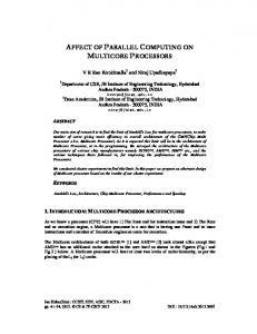
II. Plasma Stability Monitoring for Fusion Reactors 1. Motivations In this study, we have developed a high speed eigenvalue solver on a Cell cluster system, which is an essential component of a plasma stability analysis system for fusion reactors. The Japan Atomic Energy Agency (JAEA) has been developing a plasma stability analysis system, in order to achieve sustainable operation. In Fig. 1, we illustrate a schematic view of the stability analysis module in the real time plasma profile control system, which works as follows: 1. Monitor plasma current profile, pressure profile and the

author, E-mail: [email protected]

c 2011 Atomic Energy Society of Japan, All Rights Reserved.

663

Noriyuki KUSHIDA

664

boundary condition of magnetic flux surface.

Fusion Reactor

2. Calculate the plasma equilibrium using the equilibrium code.

4. If the plasma is unstable, control the pressure/current profiles to stabilize the plasma. We need to evaluate the plasma equilibrium (2.) and stability of all possible modes (3.) every two to three seconds, if the real time profile control is applied in the fusion reactors such as International Thermo-nuclear Experimental Reactor (ITER).5) The time limitation have roots in the characteristic confinement time of the density and temperature in fusion reactors; it is from three to five seconds. Moreover, we estimated that the plasma equilibrium and stability should be evaluated within half of the characteristic confinement time, by taking into account the time for data transfer, and other such activities. Since we must analyze the plasma stability within a quite short time interval, a high-speed computer is essential. The main component of the stability analysis module is the plasma simulation program MARG2D.6) MARG2D consists of roughly two parts: one is the matrix generation part, the other is the eigensolver. In particular, the eigensolver consumes the greatest amount of the computation time of MARG2D. Therefore, we focused on the eigensolver in this study. A massively parallel supercomputer (MPP), which obtains its high calculation speed by connecting many processing units and is the current trend for heavy duty computation, is inadequate for following two reasons. 1. MPPs can not be dedicated for the monitoring system. 2. MPPs have a network communication overhead. We elaborate on the above two points. Firstly, with regard to the first point, when we consider developing the plasma monitoring system, we are required to utilize a computer during the entire reactor operation. That is because fusion reactors must be monitored continuously on real time basis and immediately. For this reason, MPPs are inadequate because they are usually shared with a batch job system. Furthermore, using an MPP is unrealistic, because of its high price. Therefore, MPPs could not be dedicated to such a monitoring system. Secondly, we discuss the latter point. MPPs consist of many processing units that are connected via a network. The data transfer performance of a network is lower than that of main memory. In addition, there are several overheads that are ascribable to introducing a network, such as the time to synchronize processors, and the time to call communication functions. These overheads are typically from O(n) to O(n2 ), where n is the number of processors. Even though the overheads can be substantial with a large number of processors, they are usually negligible for large-scale computing, because the net computational time is quite long. However, the monitoring system is required to terminate within such a short period that network overheads can be dominant. Moreover, the

Data receiver

Cell cluster Cell

3. Evaluate the plasma stability for all possible modes (Plasma is stable/unstable, when the smallest eigenvalue λ, is grater/smaller than zero).

Data sender

Matrix generation Eigensolver: ~1 sec.

Controller

λ > 0: stable λ < 0: unstable

Result sender

Entire monitoring cycle: 2~3 sec. Fig. 1 Illustration of plasma stability analysis module

entire time for computation can be longer when the number of processors increases. Thus, we cannot utilize MPPs for the monitoring system. In order to solve these problems mentioned above, we introduced a Cell cluster system into this study. A cell processor is faster than a traditional processor, hence we could obtain sufficient computational power with a small number of processors. Thus, we were able to establish the Cell cluster system at much cheaper cost, and we can dedicate it to monitoring. Moreover, our Cell cluster system requires less network overhead. Therefore, it should be suitable for the monitoring system. The Cell processor obtains its greater computational power at the cost of more complex programming. Therefore, we also introduce our newly developed eigensolver in the present paper. The details of our Cell cluster system and the eigenvalue solver, are described in the following subsections (Subsections 2 and 3). Moreover, the performance is evaluated in Subection 4 and conclusions are given in Subection 5. 2. Cell Cluster (1) PowerXCell 8i PowerXCell 8i, which has a faster double precision computational unit than the original version, is a kind of Cell processor. An overview of PowerXCell 8i is shown in Fig. 2. In the figure, PPE denotes a Power PC Processor Element. The PPE has a PPU that is a processing unit equivalent to a Power PC, and also includes a second level cache memory. SPE denotes a Synergetic Processor Element, which consists of a 128 bit single instruction multiple data processing unit (hereinafter referred to as SIMD), In earlier studies,7) the processing unit was called an SPU, together with a local store (LS) and a memory flow controller (MFC), which handles data transfer between LS and main memory. The PPE, SPE, and main memory are connected with an Element Interconnect Bus (EIB). EIB has four buses and its total bandwidth reaches 204.8 Gigabytes per second. Note that the total bandwidth of EIB includes not only the data transfer between the processing unit and the main memory but also data transfer among processing units. Therefore, we usually consider the practical PROGRESS IN NUCLEAR SCIENCE AND TECHNOLOGY

On-the-Fly Computing on Many-Core Processors in Nuclear Applications

PPE

SPE SPE

SPE SPE

SPE SPE

SPE SPE

SPU

SPU

SPU

SPU

LS

LS

LS

LS

MFC

MFC

MFC

MFC

PPU L1 C ache

L2 Cach e

MIC MIC

DDR2 Main memory

Element Interconnect Bus MFC

MFC

MFC

MFC

LS

LS

LS

LS

SPU

SPU

SPU

SPU

SPE SPE

SPE SPE

SPE SPE

SPE SPE

Flex Flex IO IO

External device

Fig. 2 Overview of PowerXCell 8i processor

bandwidth of PowerXCell 8i to be 25.6 Gigabytes per second, which is the maximum access speed of main memory. (2) Cell Cluster For this study, we constructed a Cell cluster system using QS228) blades, (developed by IBM), together with the Mpich2 library. QS22 contains two Cell processors and both can access a common memory space; thus in total, sixteen SPEs are available in one QS22 blade. In addition, two QS22s are connected by a gigabit Ethernet. The Message passing interface (MPI) specification is the standard for the communication interface for distributed memory parallel computing and the Mpich2 library is one of the most well known implementations of MPI on commodity off the shelf clusters. Originally, the MPI specification was developed for a computer system with one processing unit and one main storage unit. This model is simple but not suitable for a Cell processor, because the SPUs have their own memory and therefore do not recognize a change of data in main memory. Thus, we combined two kinds of parallelization; the first is parallelization among blades using Mpich2, and the second is parallelization among SPUs. We observe, however, that a PPE only communicates to other blades using Mpich2 and SPEs do not relate to communication. Moreover, the SIMD processing unit of SPE itself is a kind of parallel processor. Then we must consider three levels of parallelization, in order to obtain better performance of the Cell cluster as follows: 1. MPI parallel 2. SPU parallel 3. SIMD parallel 3. Eigensolver Although there are numerous eigenvalue solver algorithms, only two are suitable for our purposes, because only the smallest eigenvalue is required for our plasma stability analysis system. One candidate is the Inverse power method, and the other is the conjugate gradient method (hereafter referred to as CG). The inverse power method is quite simple and easy to implement; however, it requires solving the linear equation at every iteration step, which is usually expensive in terms of time and memory. It is fortunate that the computational cost of lower/upper (LU) factorization and backward/forward (BF) substitution of block tri-diagonal matrices is linear of order n. VOL. 2, OCTOBER 2011

665

However, this is just for the sequential case. We are forced to incur additional computational cost with parallel computing, especially for MPI parallel. According to several articles, the computational cost of LU factorization increases with a small number of processors and is at least twice as great as the sequential computational cost. In our estimation, such an inflation of computational cost was not acceptable for our system. On the other hand, CG is basically well suited to distributed parallel computing, in that the computational cost for one processor linearly decreases as the number of processors that are actually used, increases. For these reasons, we employ CG as the eigenvalue solver. Details of the conjugate gradient method, including parallelization and the convergence acceleration technique that we developed are described in the following sections. (1) Preconditioned Conjugate Gradient CG is an optimization method used to minimize the value of a function. If the function is given by

f (x) =

(x, Ax) . (x, x)

(1)

The minimum value of f (x) corresponds to the minimum eigenvalue of the standard eigensystem Ax = λx, and the vector x is an eigenvector associated with the minimum eigenvalue. Here ( , ) denotes the inner product. The CG algorithm, which was originally developed by Knyazev9) and Yamada and others showed more concrete algorithm in their literature,10) (as shown in Fig. 3). In the Algorithm, T denotes the preconditioning matrix. Several variants of the conjugate gradient algorithm have been developed and have been tested for stability. According to the literature, Knyazev’s algorithm achieved quite good stability by employing Ritz method, expressed as the eigenproblem for SA v = µSB v, in the algorithm. Yamada’s algorithm is equivalent to Knyazev’s algorithm, however, it requires only one matrix-vector multiplication, which is one of the most time consuming steps of the algorithm, whereas Knyazev’s original algorithm seems require three such multiplications. Therefore, in the present study, we employ Yamada’s algorithm. Let us consider the preconditioning matrix T. The basic idea of preconditioning is to transform the coefficient matrix close to the identity matrix by operating by an inverse of T that approximates the coefficient matrix A in some sense. Even if a higher degree of approximation of T to A provides a higher convergence rate for CG, we usually stop short of achieving T = A, because the computational effort can be extremely expensive. Additionally, an inverse of T is not constructed explicitly because the computational effort can also be large. Although the matrix T−1 appears in the algorithms, the algorithm only requires solving the linear equation. We usually employ triangular matrices, or some multiples thereof, for T, because we can solve such a system with Backward/Forward (BF) substitutions. It is fortunate that complete LU factorization for block tri-diagonal matrices can be obtained at reasonable computational cost; we employed complete LU factorization to construct the preconditioning matrix T.

Noriyuki KUSHIDA

666

Cell

Cell

CPU

CPU

SPU0 SPU1 SPU2 SPU2 SPU3 SPU3 SPU4 SPU4 SPU5 SPU6 SPU7 SPU7

Cell

Cell

CPU

CPU

SPU0 SPU1 SPU2 SPU3 SPU4 SPU5 SPU6 SPU7

SPU 0 SPU 1 SPU 2 SPU 3 SPU 4 SPU 5 SPU 6 SPU 7

SPU0 SPU1 SPU2 SPU3 SPU4 SPU5 SPU6 SPU7

Traditional：

SPUs communicate regardless of communication path Hierarchical:

Slower network is used only by CPU, and faster networks is highly utilized

Giga-bit ethernet(slow) Internal network(fast) Occurred communication

Illustration of hierarchical parallelization with the comparison traditional parallelization

Fig. 4

Fig. 3 Algorithm of conjugate gradient method introduced by

Yamada et al.

(2) Parallelization of Conjugate Gradient Method As is well known, network communication can be the bottleneck in parallel computing. This is because, the bandwidth of network is much narrower than that of main memory. Therefore, we should avoid network communication as much as possible, if we need to achieve high performance. In order to reduce the amount of network communication, we employ hierarchical parallelization technique. We illustrate the comparison of hierarchical and traditional parallelization in Fig. 4. For the simplicity, we assume that two Cells are connected with Gigabit Ethernet. Note that SIMD parallelization does not appear in the figure, because SIMD parallelization is operation level parallelism and does not require communication. At the upper part of the figure, traditional parallelization is illustrated. In the traditional parallelization, each SPU communicates regardless of communication path. That is to say, they use both Gigabit Ethernet (slow: red line in the figure) and internal network (fast: blue line) at the same time, and consequently effective bandwidth becomes slower. On the other hand, SPU’s communication is strictly limited within Cell and only PPU use Gigabit Ethernet in hierarchical parallelization. By doing this, communication traffic can be reduced, and we can highly utilize the internal network. SIMD parallelization does not require communication, but is still parallel computation. It is arithmetic level parallel. Cell can compute two double precision floating-point values (FP) at one clock-cycle, while traditional processors compute one floating-point value. Therefore, Cell can process FP twice as fast as traditional processors.

4. Performance In order to investigate the performance of our eigensolver, we show the parallel performance with respect to the number of SPUs within one Cell processor Fig. 5 and the number of QS22s Fig. 6. Since the total number of SPUs in one Cell processor is 16, we measured calculation time by changing the number of SPUs from one to sixteen. These measurements were curried out by using the block tridiagonal Hermitian matrix that had 1, 024 diagonal blocks and each block size was 128 × 128. As shown in Fig. 5, we can always achieve speedup when we use larger number of SPUs. Finally, we obtained 8 times speedup at 16 SPUs. Furthermore, we can achieve speedup when we increase the number of QS22s. Even though the connection among QS22s is Gigabit Ethernet, we achieved good parallel performance (over 3times speedup at four QS22s). Therefore, it can be said that our implementation is suitable for our Cell cluster. 5. Summary for Plasma Stability Monitoring We developed a fast eigensolver on the Cell cluster. According to our evaluation, we were able to solve a block tridiagonal Hermitian matrix containing 1, 024 diagonal blocks with the relative error 1.0×10−6 , where the size of each block was 128 × 128, within a second. This performance fulfills the demand for monitoring.

III. Infrasound Monitoring 1. Motivations Verification of the Comprehensive Nuclear-test-ban Treaty (CTBT) requires the ability to detect, localize, and discriminate nuclear events on a global scale.11) Monitoring and assessing infrasound propagations are one of ways to achieve the purpose. Many propagation analysis programs have been developed for this purpose. One of these programs called InfraMAP. The main functionality of InfraMAP is simulating the propagation paths of infrasound by using several simulation programs. From this standpoint, InfraMAP equips three simulation methods: Normal mode (NM), Ray-trace, (RT) and PROGRESS IN NUCLEAR SCIENCE AND TECHNOLOGY

On-the-Fly Computing on Many-Core Processors in Nuclear Applications

Speed-up Ratio

Elaspsed Time

14

ATI Radeon 5870

16

8

4

Speed-up Ratio

Elapsed Time ( sec. )

10

6

2 0

1 2

4

8

Number of SPUs

Compute Unit 20

Compute Unit 2 Compute Unit 1

12

8

667

Proc. Elem. 1 Local Data Storage (LS)

Proc. Elem. 16

Proc. Elem. 1

Read/Write Memory

1 16

Local Data Storage (LS)

Data Cache

Proc. Elem. 16

Data Cache

Read Only Memory

Host Device (x86 PC)

Fig. 5 Parallel performance with respect to the number of

SPUs within one Cell Elapsed Time

1.6

Fig. 7 Configuration of HD5870

Speed-up Ratio

4

1.2

3

1 0.8 0.6

2

0.4

Speed-up Ratio

Elapsed Time ( sec. )

1.4

2. GPGPU -ATI Radeon HD5870-

0.2 0

Therefore, we accelerate the PE method by using GPGPU, which recently becomes famous its high computational speed and low price. In this study, we aim to reduce the calculation time of PE to that of RT on CPU, in order to obtain more accurate result than RT in the same calculation time of RT. Typically, RT is ten times faster than PE, and therefore our target performance is ten times better performance than one CPU.13)

1

2 3 Number of QS22s

4

1

Fig. 6 Parallel performance with respect to the number of

QS22s

Parabolic equation (PE) method. Each has its own advantages and disadvantages. Among other things, PE is the strongest method when we analyze detailed propagation path of infrasound. This is because PE method yields the solution to a discretized version of the full acoustic wave equation for arbitrarily complex media.12) It is a full spectrum approach and is thus reliable at all angles of propagation, including backscatter. This offers an advantage over other standard propagation methods in wide use, as it allows for accurate computation of acoustic energy levels in the case where significant scattering can occur near the source, such as may happen for an explosion near the surface, or under ground. This fits in with nuclear monitoring goals in that it allows for an improved understanding of the generation and propagation of infrasound energy from underground and near-surface explosions. However, PE requires much higher computational power than others do, while such analysis is curried out on a workstation. VOL. 2, OCTOBER 2011

We employed ATI Radeon HD5870 as an accelerator device. It is a kind of GPGPU. The configuration of HD5870 is shown in Fig. 7. HD5870 has 1 GByte memory that consists of read/write area and read only area, and has 20 compute units (CU). Each CU has 16 processor elements, 32 KByte locate date storage (LS), and 16 KByte cache. A processor element includes five single precision arithmetic logic units (ALU). The total performance reaches 2.7 TFLOPS. The bandwidth of memory is 154 GByte/sec, and can be limit the entire performance of scientific computing. In order to fill the gap, CU has LS. LS is scratch pad memory and has 2 TByte/sec bandwidth. This situation is quite similar to the Cell’s situation. Additionally, data cache that works only with read only memory has 1 TByte/sec bandwidth, and it works independently from LS. 3. Governing Equations and Discretization In order to analyze the propagation path of infrasound on inhomogeneous moving media, we employ Ostashev et al.’s model.14) The resulted partial differential equations in twodimensional case are, ∂p ∂t

( ) ( ) ∂ ∂ ∂wx ∂wy = − vx + vy −κ + ∂x ∂y ∂x ∂y +κQ, (2)

Noriyuki KUSHIDA

668

∂wy ∂t

( ) ( ) ∂ ∂ ∂ ∂ = − wx + wy vx − vx + vy wx ∂x ∂y ∂x ∂y ∂p −b + bFx , (3) ∂x ( ) ( ) ∂ ∂ ∂ ∂ = − wx + wy vy − vx + vy wy ∂x ∂y ∂x ∂y ∂p −b + bFy , (4) ∂y

where, p, wx , and wy , are the pressure and velocity of infrasound, and vx , and vy are the velocity of wind, respectively. Further, b = 1/ρ where ρ is density of atmosphere, and κ = ρc2 , where c is adiabatic sound speed. Fx , Fy , and Q are the external sources of infrasound. These equations are discretized by using finite difference method (FDM) with staggered grid. Moreover, fourth order explicit Runge-Kutta scheme is employed for time development. 4. Pipelining Method and Memory Configuration Optimization Because of the big gap between computational power and memory bandwidth, we must utilize LS and data cache to achieve high performance. In order to utilize LS, we employ the software-pipelining method developed by Watanabe et al.15) We show the memory layout and data flow of softwarepipelining method in Fig. 8 . Each LS has only 32 KByte and cannot store entire data, if all LS divide the entire domain. Therefore, we assign small partition of analysis domain on LS. If additional new data are needed, they are sent to LS but old data are kept during they are useful. Thanks to the Watanabe’s method, we can reduce over 60% of memory access to main memory. HD5870 has vector data type, which contains four floating-point values in one variable. Since HD5870 is optimized handling vector data, we can obtain better performance by using it. In order to use the vector data type, we pack several field data to a vector data. For example, p(i, j), wx (i, j), and wy (i, j), are stored in the same variable, where (i, j) denotes the grid point. Furthermore, we assign background data (vx , vy ,ρ,c, and Q) on read only memory, in order to utilize data cache and reduce the effective load of memory bandwidth. 5. Performance Evaluation In order to evaluate the performance of our implementation, we measured FLOPS and calculation time of HD5870 and CPU (Intel Xeon X5570 2.93 GHz). In Table 1, we tabulate the GFLOPS and calculation time of each implementation. We prepared two sizes of FDM grids: nx = 1, 024, ny = 1, 024, and nx = 2, 560, ny = 1, 024, where nx, and ny are the number of grid points along x and y axis, respectively. In the table, CPU denotes CPU implementation, Pipelining denotes Pipelining method on GPU, Vector data denotes optimization by using vector data type for pipelining method, and Read only denotes that optimization by using read only memory data area for background variables on Vector data. GFLOPS on CPU was obtained by using performance counter. GFLOPS of GPU implementations were calculated based on the result of CPU. When we see the re-

LS1

LS2

LS20

Repeat until y ends

∂wx ∂t

: Data Newly loaded

Entire Analysis Domain

y

: Data stored on LS : Data dropped

x

Fig. 8 Memory layout and data flow of software-pipelining

method by Watanabe et al.

Table 1 GFLOPS and Calculation time of each implementa-

tion

CPU Pipelining Vector data Read only

1,024 × 1,024 GFLOPS TIME(sec) 2.66E+00 15.77 1.17E+01 3.59 1.37E+01 3.07 1.53E+01 2.74

2,560 × 1,024 GFLOPS TIME(sec) 2.09E+00 50.35 2.93E+01 3.59 3.46E+01 3.05 3.83E+01 2.75

sult of CPU, the more grid points we use, the worse GFLOPS we obtained. This is because cache memory of CPU becomes ineffective when the number of grid increases. On the other hand, GPU implementations do not show the difference between two grids. The reason why we cannot observe the difference is that we could not utilize all of CU in smaller problem and the rest of them just slept during calculation. This result would be observed until nx reaches to 2, 560. According to our estimation, all the CU can work only at nx = 2, 560 and shows the best performance on our implementation. Calculation speed of GPU is originally better than that of CPU. Additionally, when we applied optimization, we could accelerate 1.5 times. Finally, we obtained ×18.3 speed-up on GPU than CPU in larger problem. 6. Summary for Infrasound Propagation Analysis We implemented the simulation program of infrasound propagation on both CPU and GPU. It was based on Ostashev’s model and was discretized by FDM. GPU implementation was optimized by using the pipelining method, the vector data type, and the read only memory. Finally, we obtained ×18.3 speed-up from CPU, which was above our initial objective. PROGRESS IN NUCLEAR SCIENCE AND TECHNOLOGY

On-the-Fly Computing on Many-Core Processors in Nuclear Applications

IV. Conclusion In this study, we achieved speed-up in two nuclear applications by using computer accelerators. One is plasma stability analysis on Cell cluster, and the other is infrasound propagation simulation on GPGPU. In plasma stability analysis, we could solve a tri-diagonal Hermitian matrix within one second, which contains 1, 024 diagonal blocks where the size of each block was 128×128. On the other hand, infrasound propagation simulation, we could achieve ×18.3 speedup from CPU in PE method by using GPGPU. PE has not been preferred because of its large computational requirements, so far. However, time cost of PE and RT is almost same now. We hope that our implementation brings result that is more accurate than current result for CTBT.

5) 6)

7) 8) 9)

10)

Acknowledgment

11)

We are grateful to JSPS for the Grant-in-Aid for Young Scientists (B), No. 21760701. We also thank A. Tomita and K. Fujibayashi FIXSTARS Co. for their extensive knowledge of the CELL, and Dr. M. Segawa for her sound advice on writing.

12)

References

13)

1)

2)

3) 4)

J. Gebis, L. Oliker, J. Shalf, S. Williams, K. Yelick, “Improving Memory Subsystem Performance using ViVA: Virtual Vector Architecture”, ARCS: International Conference on Architecture of Computing Systems, Delft, Netherlands, March (2009). International Business Machines Corporation, Sony Computer Entertainment Incorporated, and Toshiba Corporation, Cell Broadband Engine Architecture, Version 1.01 (2006). Advanced Mircro Technology, ATI Stream SDK OpenCL Programming Guide (2010). Top500 supercomputer sites, http://www.top500.org (2010).

VOL. 2, OCTOBER 2011

14)

15)

669

ITER project web page, http://www.iter.org/default.aspx (2010). S. Tokuda, T. Watanabe, “A new eigenvalue problem associated with the two-dimensional Newcomb equation without continuous spectra,” Phys. Plasmas, 6[8], 3012–3026, (1999). M. Scarpino, Programming the Cell procssor for Games, Graphics, and Computation, Pearson Education (2009). Prodcut information of QS22, available at http://www-03. ibm.com/systems/info/bladecenter/qs22/. A. V. Knyazev, “Toward the optimal eigensolver: Locally optimal block preconditioned conjugate gradient method,” SIAM J. Sci. Comput., 23, 517–541, (2001). S. Yamada, T. Imamura, M. Machida, “Preconditioned Conjugate Gradient Method for Largescale Eigenvalue Problem of Quantum Problem,” Trans. JSCES, No. 20060027 (2006), [In Japanese]. R. Gibson, D. Norris, T. Farrell, “Development and Application of an Integrated Infrasound Propagation Modeling Toll Kit,” 21st Seismic Research Symposium, 112–122 (1999). C. Groot-Hedlin, “Finite Difference Modeling of Infrasound Propagation to Local and Regional Distances,” 29th Monitoring Research Review: Ground-Based Nuclear Explosion Monitoring Technologies, 836–844 (2007). P. Bernardi, M. Cavagnaro, P. D’Atanasio, E. Di Palma, S. Pisa, E. Piuzzi, “FDTD, multiple-region/FDTD, ray-tracing/ FDTD: acomparison on their applicability for human exposure evaluation,” Int. J. Numer. Model, 15, 579–593 (2002). V. E. Ostashev et al., “Equations for finite-difference, timedomain simulation of sound propagation in moving inhomogeneous media and numerical implementation,” J. Acoust. Soc. Am., 117[2], 503–517 (2005). S. Watanabe, O. Hashimoto, “An Examination about Speedup of 3 Dimensional Finite Difference Time Domain (FDTD) Method Using Cell Broadband Engine (Cell/B.E.) Processor,” IEICE Technical Report, 109, 1–6 (2009), [In Japanese].