On the frequentist validity of Bayesian limits

See discussions, stats, and author profiles for this publication at: https://www.researchgate.net/publication/310953267

On the frequentist validity of Bayesian limits Article · November 2016

CITATIONS

READS

0

4

1 author: B. J. K. Kleijn University of Amsterdam 22 PUBLICATIONS 479 CITATIONS SEE PROFILE

Some of the authors of this publication are also working on these related projects:

Bayesian limit theorems for frequentists View project

All content following this page was uploaded by B. J. K. Kleijn on 31 December 2016. The user has requested enhancement of the downloaded file. All in-text references underlined in blue are added to the original document and are linked to publications on ResearchGate, letting you access and read them immediately.

On the frequentist validity of Bayesian limits B. J. K. Kleijn Korteweg-de Vries Institute for Mathematics, University of Amsterdam

arXiv:1611.08444v1 [math.ST] 25 Nov 2016

November 2016, version 0.6 Abstract Four frequentist theorems on the large-sample limit behaviour of posterior distributions are proved, for posterior consistency in metric or weak topologies; for posterior rates of convergence in metric topologies; for consistency of the Bayes Factor for hypothesis testing or model selection; and a new theorem that explains how credible sets are to be transformed to become asymptotic confidence sets. Proofs require the existence of suitable test sequences and priors that give rise to a property of local prior predictive distributions called remote contiguity, which generalizes Schwartz’s Kullback-Leibler condition as a weakened form of Le Cam’s contiguity. Results are applied in a range of examples and counterexamples.

1

Introduction

The work presented here should be of interest both to the frequentist with an interest in Bayesian asymptotics, and to the Bayesian that has an eye for asymptotic, frequentist arguments. Following Bayarri and Berger (2004) [3] (”Statisticians should readily use both Bayesian and frequentist ideas.”), we illustrate how Bayesian asymptotic conclusions can be converted into conclusions valid in the frequentist sense: how Doob’s prior-almostsure consistency is supplemented to reach the frequentist conclusion that the posterior is consistent, or how a Bayesian credible set has to be enlarged in order for it to become a frequentist confidence set, for example. The central property imposed on the prior that allows frequentist interpretation of Bayesian asymptotics, defined as remote contiguity in subsection 3.1, expresses a weakened form of Le Cam’s contiguity, relating the true distribution of the data to localized prior predictive distributions. Where Schwartz’s Kullback-Leibler neighbourhoods represent a choice for the localization appropriate when the sample is i.i.d., remote contiguity generalizes the notion to include non-i.i.d. samples, priors that change with the sample size, weak consistency with the Dirichlet process prior, etcetera. Although this work firstly concerns generalization and simplification in well-studied asymptotic questions, it also has a novel and very practical consequence: the fourth 1

theorem in section 4 demonstrates in full generality that credible sets can be ‘enlarged’ in a way prescribed by remote contiguity, to convert them to asymptotically consistent confidence sets. So the asymptotic validity of credible sets as confidence sets implied by the Bernstein-von Mises theorem extends much further: to find asymptotic confidence sets in practice, the frequentist can (MCMC-)simulate posteriors and ‘enlarge’ resulting (HPD-)credible sets if he uses a prior that induces the right type of remote contiguity. In the subsection that follows, we formulate the posterior consistency question and present some early answers as well as counterexamples and related problems. In section 2 we concentrate on an inequality expressing asymptotic concentration of posterior mass if a test sequence exists and indicate the relation with Le Cam’s inequality [33]. Section 3 introduces remote contiguity and the analog of Le Cam’s First Lemma. In section 4, four frequentist theorems on the asymptotic behaviour of posterior distributions are proved, on posterior consistency, on posterior rates of convergence, on consistent testing and model selection with Bayes factors and on the conversion of credible sets to confidence sets. Section 5 discusses future directions. Definitions, notation, conventions and other preliminaries have been collected in appendix A. In particular remarks A.1 and A.4 describe general assumptions that apply throughout this paper. All proofs can be found in appendix E.

1.1

Posterior consistency and inconsistency

Consider a model P for data with true distribution P0 with given Hausdorff topology: we say that a Borel prior Π on P gives rise to posterior distributions consistent at P0 , if every neighbourhood of P0 receives posterior mass one asymptotically (see definition 4.1). The first general consistency theorem is due to Doob. Theorem 1.1 (Doob (1949) [14]) Suppose that we have i.i.d. data X1 , X2 , . . . ∈ X and a model P of single-observation distributions P0 . Suppose X and P are Polish spaces. Assume that P 7→ P (A) is Borel measurable for every Borel set A ⊂ X . Then for any prior Π on P the posterior is consistent, for Π-almost-all P0 . In parametric applications Doob’s Π-null-set of possible inconsistency can be considered ‘small’ (for example, when the prior dominates Lebesgue measure). But in nonparametric context these null-sets can be very large (or not, see [37]): the first nonparametric examples of unexpected inconsistency of the posterior are due to Schwartz (1961) [39], but it was Freedman who made the point famous with a simple nonparametric counterexample that is discussed in some detail as example D.1. The implication was that certain choices for the prior could lead to unforeseen instances of

2

inconsistency. But Freedman’s construction required knowledge of the true distribution of the data, so it was possible to argue that his counterexample amounted to the demonstration that unfortunate circumstances could be created, but were probably not of great concern in a more generic sense. Two years later, Freedman constructed priors of the problematic type without knowing the true distribution of the data. In fact, he went further and showed that inconsistency is generic in a topological sense. Theorem 1.2 (Freedman (1965) [17]) Let X1 , X2 , . . . form an sample of i.i.d.-P0 integers, let Λ denote the space of all distributions on N and let π(Λ) denote the space of all Borel probability measures on Λ, both in Prokhorov’s weak topology. The set of pairs (P0 , Π) ∈ Λ × π(Λ) such that for all open U ⊂ Λ, lim sup P0n Π(U |X n ) = 1, n→∞

is residual. So Freedman’s theorem says that posteriors that continue to wander around, placing and re-placing mass aimlessly, are the rule rather than the exception and the set of pairs (P0 , Π) ∈ Λ × π(Λ) for which the posterior is consistent is meagre in Λ × π(Λ). Many conclusions have been drawn from these and subsequent examples of posterior inconsistency, the most damaging of which was wide-spread acceptance among frequentists that Bayesian methods were generically unfit for frequentist purposes, at least in non-parametric context. The only justifiable conclusion from Freedman’s meagreness is that there is a condition missing: Doob’s assetion may be all that a Bayesian requires, a frequentist demands strictly more, thus restricting the class of possible choices for his priors. So when the goal is the frequentist asymptotic use of posteriors, an additional condition for the prior is required. When Freedman’s meagreness result was published a condition this type had already been found. Theorem 1.3 (Schwartz (1965)) For all n ≥ 1, let (X1 , X2 , . . . , Xn ) ∈ X n be i .i .d . − P0 and let U denote an open neighbourhood of P0 . If, (i) there exists a sequence of measurable φn : X n → [0, 1], such that, P0n φn = o(1),

sup Qn (1 − φn ) = o(1),

Q∈U c

(ii) and Π is a Kullback-Leibler prior, i.e. for all δ > 0,   dP < δ > 0, Π P ∈ P : −P0 log dP0

(1)

P -a.s.

then Π(U |X n ) −−0−−→ 1. Over the decades, examples of problematic posterior behaviour in non-parametric setting continued to attract attention [10, 11, 8, 12, 13, 18, 19], while Schwartz’s theorem remaied 3

the foundation for much of Bayesian non-parametric asymptotics: subsequent frequentist theorems (e.g. by Barron (1988) [1], Barron-Schervish-Wasserman (1999) [2], GhosalGhosh-van der Vaart (2000) [21], Shen-Wasserman (2001) [41], Walker (2004) [45] and Walker-Lijoi-Pr¨ unster (2007) [47], Kleijn-Zhao (2016) [27] and others) have extended the applicability of theorem 1.3 but not its essence, condition (1) for the prior. The following example illustrates that Schwartz’s condition cannot be the whole truth, though. Example 1.4 Consider X1 , X2 , . . . that are i.i.d.-P0 with Lebesgue density p0 : R → R supported on an interval of known width (say, 1) but unknown location. Parametrize in terms of a continuous density η on [0, 1] with η(x) > 0 for all x ∈ [0, 1] and a location θ ∈ R: pθ,η (x) = η(x − θ) 1[θ,θ+1] (x). A moment’s throught makes clear that if θ 6= θ0 , −Pθ,η log

pθ0 ,η0 =∞ pθ,η

for all η, η 0 . Therefore Kullback-Leibler neighbourhoods do not have any extent in the θ-direction and no prior is a Kullback-Leibler prior in this model. Nevertheless posterior consistency obtains (see examples D.8 and D.9).



Similar counterexamples exist for the type of prior Ghosal et al. [21] and Shen-Wasserman [41] propose in their analyses of posterior rates of convergence in (Hellinger) metric setting. Although methods in [27] avoid this type of problem, the essential nature of condition (1) in i.i.d. setting becomes apparent there as well. For other central asymptotic questions, insightful answers remain elusive: why is Doob’s theorem completely different from Schwartz’s? The accepted perspective explains the lack of congruence as an indistinct symptom of fundamental philosophical differences between the Bayesian and Frequentist schools, but is this justified? Why does weak consistency in the full non-parametric model (e.g. with the Dirichlet process prior [15], or more modern variations [9]) reside in a corner of its own (with tailfreeness [17] being the sufficient property of the prior), apparently unrelated to posterior consistency in either Doob’s or Schwartz’s views? Indeed, what would Schwartz’s theorem look like without the assumption that the sample is i.i.d. (e.g. with dependent data that realizes a stochastic process, with growing parameter spaces or with changing priors, etcetera)? And to extend the scope further, what can be said about hypothesis testing, classification, model selection, etcetera? Given that the Bernstein-von Mises theorem cannot be expected to hold in any generality outside parametric setting [8, 19], what relationship exists between credible sets and confidence sets? This paper aims to shed more light on these questions in a general sense, by providing a prior condition that enables strengthening Bayesian asymptotic conclusions to frequentist ones.

4

2

Posterior concentration and asymptotic tests

In this section, we consider a lemma that relates concentration of posterior mass in certain model subsets to the existence of test sequences that distinguish between those subsets. More precisely, it is shown that the expected posterior mass outside a model subset V with respect to the local prior predictive distribution over a model subset B, is upper bounded (roughly) by the testing power of any statistical test for the hypotheses B versus V : if a test sequence exists, the posterior will concentrate its mass appropriately.

2.1

Bayesian test sequences

Since the work of Schwartz [40], test sequences and posterior convergence have been linked intimately. In this paper, we follow Schwartz and consider asymptotic testing; however, we define test sequences immediately in Bayesian context by involving priors from the outset. Definition 2.1 Given priors (Πn ), measurable model subsets (Bn ), (Vn ) ⊂ G and an ↓ 0, a sequence of Bn -measurable maps φn : Xn → [0, 1] is called a Bayesian test sequence for Bn versus Vn (under Πn ) of power an , if, Z Z n Pθ,n (1 − φn (X n )) dΠn (θ) = o(an ). Pθ,n φn (X ) dΠn (θ) + Bn

(2)

Vn

We say that (φn ) is a Bayesian test sequence for Bn versus Vn (under Πn ) if (2) holds for some an ↓ 0. Note that if we have sequences (Cn ) and (Wn ) such that Cn ⊂ Bn and Wn ⊂ Vn for all n ≥ 1, then a Bayesian test sequence for (Bn ) versus (Vn ) under Π of power an is a Bayesian test sequence for (Cn ) versus (Wn ) under Π of power (at least) an . Bayesian test sequences and concentration of the posterior are related through the following lemma (in which n-dependence is suppressed for clarity). Lemma 2.2 For any B, V ∈ G with Π(B) > 0 and any measurable φ : X → [0, 1], Z Z Z 1 Pθ (1 − φ(X)) dΠ(θ). Pθ Π(V |X) dΠ(θ|B) ≤ Pθ φ(X) dΠ(θ|B) + Π(B) V

(3)

Thus, the existence of test sequences is enough to guarantee posterior concentration, a fact expressed in suitable, n-dependent form through the following proposition. Proposition 2.3 Assume that for given priors Πn , sequences (Bn ), (Vn ) ⊂ G and an , bn ↓ 0 such that an = o(bn ) with Πn (Bn ) ≥ bn > 0, there exists a Bayesian test sequence for Bn versus Vn of power an . Then for all n ≥ 1, PnΠn |Bn Πn (Vn |X n ) = o(an b−1 n ). 5

(4)

To see how this leads to posterior consistency, consider the following: if the model subsets Vn = V are all equal to the complement of a neighbourhood of P0 , and the Bn are chosen such that the expectations of the random variables X n 7→ Πn (V |X n ) under Π |Bn

Pn n

‘dominate’ their expectations under P0,n in a suitable way, sufficiency of prior

mass bn given testing power an ↓ 0, is enough to assert that P0,n Πn (V |X n ) → 0.

2.2

The existence of test sequences

An application of Hoeffding’s inequality demonstrates that, for any weak neighbourhoods (see definition C.1), are uniformly testable. Proposition 2.4 (Uniform weak (Tn -)tests) Consider a model P of distributions P for i.i.d. data (X1 , X2 , . . . , Xn ) ∼ P n , (n ≥ 1). Let  > 0, P0 ∈ P and a measurable f : X n → [0, 1] be given. Define,  B = P ∈ P : |(P n − P0n )f | <  ,

 V = P ∈ P : |(P n − P0n )f | ≥ 2 .

There exist a D > 0 and uniform test sequence (φn ) such that, sup P n φn ≤ e−nD ,

sup Qn (1 − φn ) ≤ e−nD .

P ∈B

Q∈V

Another well-known example concerns testability of convex model subsets. The uniform test sequences in Schwartz’s theorem are constructed using building convex blocks B and V of distributions separated in Hellinger distance. Proposition 2.5 (Minimax Hellinger tests) Consider a model P of distributions P for i.i.d. data (X1 , X2 , . . . , Xn ) ∼ P n , (n ≥ 1). Let B, V ⊂ P be convex with H(B, V ) > 0. There exist a test sequence (φn ) such that, 1

sup P n φn ≤ e− 2 n H P ∈B

2 (B,V

)

1

,

sup Qn (1 − φn ) ≤ e− 2 n H

2 (B,V

)

.

Q∈V

Questions concerning consistency require the existence of tests in which at least one of the two hypotheses is a non-convex set, typically the complement of a neighbourhood. Imposing the model P to be of bounded entropy with respect to the Hellinger metric allows construction of such tests, based on the uniform tests of proposition 2.5. (For more on this construction, see Le Cam (1973) [32], Birg´e (1983,1984) [4, 5] and example D.4.) It is worth pointing out at this stage that posterior inconsistency due to the phenomenon of ‘data tracking’ [2, 46], whereby weak posterior consistency holds but Hellinger consistency fails, can only be due to failure of the extra entropy condition needed for the construction of tests in the Hellinger case. The existence of Bayesian test sequences c.f. (2) is linked directly to behaviour of the posterior. 6

Theorem 2.6 Let (P, G , Π) be given. For any B, V ∈ G , the following are equivalent, (i) There exist tests (φn ) such that, Z Z Qn (1 − φn ) dΠ(Q) → 0, P n φn dΠ(P ) + V

B

(ii) For Π-almost-all P ∈ B, Q ∈ V , P -a.s.

Π(V |X n ) −−−−→ 0,

Q-a.s.

Π(B|X n ) −−−−→ 0.

The interpretation of this theorem is gratifying to supporters of the likelihood principle and pure Bayesians: distinctions between model subsets are Bayesian testable, if and only if, they are picked up by the posterior asymptotically, if and only if, the Bayes factor for B versus V is consistent. To illustrate how essential the existence of Bayesian test sequences is, note the following lemma. Lemma 2.7 Suppose that (Θ, d) is a metric space and that θˆn : Xn → Θ is consistent, that is, θˆn converges to θ in Pθ,n -probability. Then, for every θ0 ∈ Θ and  > 0 there exists a Bayesian test sequence for B = {θ ∈ Θ : d(θ, θ0 ) < 21 } versus V = {θ ∈ Θ : d(θ, θ0 ) > }. For our present purposes, it is important to note that theorem 2.6 implies Doob’s consistency theorem because of the following lemma. Lemma 2.8 Consider a model P of single-observation distributions P for i.i.d. data (X1 , X2 , . . . , Xn ) ∼ P n , (n ≥ 1). Assume that P is a Polish space with Borel prior Π. For any Borel set V there exists a Bayesian test sequence for V versus P \ V under Π. Given a sample X1 , X2 , . . . that is i.i.d.-P0 , one substitutes any open neighbourhood U of P0 for P \ V and B = U in lemma 2.8 to arrive at Doob’s theorem 1.1 through theorem 2.6. In subsection D.2 we consider another construction of a Bayesian test sequence, which combines aspects of example D.4 with an argument due to Barron [1] concerning priors on parameter spaces that are not pre-compact in the Hellinger topology. The construction allows control over the power of Bayesian tests, as required in the theorems of section 4.

2.3

Le Cam’s inequality

Referring to the last sentence in subsection 2.1, one way of guaranteeing that the expecΠ|Bn

tations of X n 7→ Πn (V |X n ) under Pn

approximate their expectations under P0,n , is

to assume that the model is well-specified and choose the Bn equal to total-variational balls around the points Pθ0 ,n , Bn = {θ ∈ Θ : kPθ,n − Pθ0 ,n k ≤ δn }, 7

for some sequence δn → 0, because in that case, Z n P0,n ψ(X ) ≤ + P0,n ψ(X ) − Pθ,n ψ(X n ) dΠ(θ|Bn ) Z Π|Bn n ≤ Pn ψ(X ) + kPθ,n − P0,n k dΠ(θ|Bn ) ≤ PnΠ|Bn ψ(X n ) + δn n

PnΠ|Bn ψ(X n )

for any random variable ψ : Xn → [0, 1]. Without fixing the definition of the sets Bn , one may use the step in the display above to specify inequality (3) further:

P0,n Πn (Vn |X) ≤ P0,n − PnΠ|Bn Z Z Πn (Vn ) + Pθ,n φn (X) dΠn (θ|Bn ) + Pθ,n (1 − φn (X)) dΠn (θ|Vn ), Πn (Bn )

(5)

for Bn and Vn such that Πn (Bn ) > 0 and Πn (Vn ) > 0. Le Cam’s inequality (5) is used, for example, in the proof of the Bernstein-von Mises theorem, see lemma 2 in section 8.4 of [36]. A less successful application pertains to non-parametric posterior rates of convergence for i.i.d. data, in an unpublished paper (Le Cam (197X) [33]). Rates of convergence obtained in this way are suboptimal: Le Cam qualifies the first term on the right-hand side of (5) as a “considerable nuisance” and concludes that “it is unclear at the time of this writing what general features, besides the metric structure, could be used to refine the results”, (see [34], end of section 16.6). In [49], Le Cam relates the posterior question to dimensionality restrictions [32, 41, 21] and reiterates, “And for Bayes risk, I know that just the metric structure does not catch everything, but I don’t know what else to look at, except calculations.”

3

Remote contiguity

Contiguity describes an asymptotic version of absolute continuity, applicable to sequences of probability measures in a limiting sense (Le Cam (1960) [31]). A condensed overview of the most basic characterizations of contiguity and some essential references are found in appendix B. In this section we weaken the property in a way that is suitable to promote Π-almost-everywhere, Bayesian limits to frequentist ones, valid for all model distributions.

3.1

Definition and criteria for remote contiguity

The notion of ‘domination’ left undefined in the last sentence in subsection 2.1 is made rigorous here. Definition 3.1 Given measurable spaces (Xn , Bn ), n ≥ 1 with two sequences (Pn ) and (Qn ) of probability measures and a sequence ρn ↓ 0, we say that Qn is ρn -remotely

8

contiguous with respect to Pn , notation Qn C ρ−1 n Pn , if, Pn φn (X n ) = o(ρn )

⇒

Qn φn (X n ) = o(1).

for every sequence of Bn -measurable φn : Xn → [0, 1]. Note that given two sequences (Pn ) and (Qn ), contiguity Pn CQn is equivalent to remote contiguity Pn C a−1 n Qn for all an ↓ 0. Given sequences an , bn ↓ 0 with an = o(bn ), bn remote contiguity implies an -remote contiguity of (Pn ) with respect to (Qn ). Example 3.2 Let P be a model for the distribution of a single observation from i.i.d. samples X n = (X1 , . . . , Xn ). Let P0 , P and  > 0 be such that −P0 log(dP/dP0 ) < 2 . The law of large numbers implies that for large enough n, n 2 dP n n (X ) ≥ e− 2  , n dP0

(6)

with P0n -probability one. Consequently, for large enough n and for any Bn -measurable sequence ψn : Xn → [0, 1], n 2

P n ψn ≥ e− 2  P0n ψn , Therefore, if P n φn = o(exp (− 12 n2 )) then P0n φn = o(1). Conclude that for every  > 0, the Kullback-Leibler neighbourhood B() = {P : −P0 log(dP/dP0 ) < 2 } consists of model distributions for which the sequence (P0n ) of product distributions are exp (− 21 n2 )-remotely contiguous with respect to (P n ).



Criteria for remote contiguity are given in the lemma below; note that, here, we give sufficient conditions (rather than necessary and sufficient, as in lemma B.2). Lemma 3.3 Given (Pn ), (Qn ), an ↓ 0, Qn C a−1 n Pn , if any of the following hold: P

Qn

n (i) For any Bn -measurable φn : Xn → [0, 1], a−1 −→ 0 implies that φn −−→ 0; n φn −

(ii) Given  > 0, there is a constant δ > 0 s.t. Qn (dPn /dQn < δ an ) < , f.l.e.n.; −1 (iii) There is a constant b > 0 s.t. lim inf n b a−1 n Pn (dQn /dPn > b an ) = 1;

(iv) Given  > 0, there is a c > 0 s.t. kQn − Qn ∧ c a−1 n Pn k < , f.l.e.n.; (v) Under Qn , (an dQn /dPn ) is a sequence of random variables s.t. every subsequence has a weakly convergent subsequence; Proof The proof of this lemma can be found in appendix E. It actually proves that ((i) or (iv)) implies remote contiguity; that ((ii) or (iii)) implies (iv)and that (v) is equivalent to (ii).



Note that for (Qn ) that is an -remotely contiguous with respect to (Pn ), there exists no test that distinguishes between Pn and Qn with power an .

9

3.2

Remote contiguity for Bayesian limits

The relevant applications in the context of Bayesian limit theorems both concern remote contiguity of the sequence of true distributions Pθ0 ,n with respect to local prior predictive Π |Bn

distributions Pn n

, where the sets Bn ⊂ Θ are such that, Πn |Bn Pθ0 ,n C a−1 , n Pn

(7)

for some rate an ↓ 0. Π |Bn

According to lemma 3.3-(v), (7) holds if the likelihood ratios Zn = dPθ0 ,n /dPn n

(X n )

satisfy Pθ0 ,n (Zn < ∞) = 1 (n ≥ 1), and have a weak limit Z when re-scaled by an , Pθ

,n -w.

0 an Zn −−− −−→ Z. To better understand the counterexamples of subsection D.1, notice

the high sensitivity of this criterion to the existence of subsets of the sample spaces assigned probability zero under model distributions, while the true probability is non-zero. More generally, remote contiguity is sensitive to subsets En assigned fast decreasing Π |Bn

probabilities under local prior predictive distributions Pn n

(En ), while the probabili-

ties Pθ0 ,n (En ) remain high, which is what definition 3.1 expresses. The rate an ↓ 0 helps to control the likelihood ratio (compare to the unscaled limits of likelihood ratios that play a central role in the theory of convergence of experiments [34, 36]), conceivably enough to force uniform tightness in non-parametric situations. But condition (7) can also be written out, for example to the requirement that for some constant δ > 0,  Z dP  θ,n (X n ) dΠn (θ|Bn ) < δ an → 0, Pθ0 ,n dPθ0 ,n with the help of lemma 3.3-(ii). Example 3.4 Consider again the model of example 1.4. In example D.8, it is shown that if the prior Π for θ ∈ R has a continuous and strictly positive Lebesgue density and we choose Bn = [θ0 , θ0 + 1/n], then for every δ > 0 and all an ↓ 0, Z 
dPθ,n Pθn0 (X n ) dΠn (θ|Bn ) < δ an ≤ Pθn0 n(X(1) − θ0 ) < 2δ an dPθ0 ,n for large enough n ≥ 1, and the r.h.s. goes to zero for any an because the random variables n(X(1) − θ0 ) have a non-degenerate weak limit under Pθn0 as n → ∞. Conclude that with these choices for Π and Bn , (7) holds, for any an .



The following proposition should be viewed in light of Le Cam and Yang (1988) [35], which considers properties like contiguity, convergence of experiments and local asymptotic normality in situations of statistical information loss. In this case, we are interested in (remote) contiguity of the probability measures that arise as marginals for the data X n when information concerning the (Bayesian random) parameter θ is unavailable.

10

Proposition 3.5 Let θ0 ∈ Θ and a prior Π : G → [0, 1] be given. Let B be a measurable subset of Θ such that Π(B) > 0. Assume that for some an ↓ 0, the family,   dPθ0 ,n n an (X ) : θ ∈ B, n ≥ 1 dPθ,n Π|B

is uniformly tight under Pθ0 ,n . Then Pθ0 ,n C a−1 n Pn

.

Other sufficient conditions from lemma 3.3 may replace the uniform tightness condition. When the prior Π and subset B are n-dependent, application of lemma 3.3 requires more. (See, for instance, example D.17 and lemma D.18, where local asymptotic normality is used to prove (7).) If remote contiguity of the type (7) can be achieved for a sequence of subsets (Bn ), then it also holds for any sequence of sets that contain the Bn but at a rate that differs proportionally to the fraction of prior masses. Lemma 3.6 For all n ≥ 1, let Bn ⊂ Θ be such that Πn (Bn ) > 0 and Cn such that Bn ⊂ Cn with cn = Πn (Bn )/Πn (Cn ) ↓ 0, then, Πn |Cn . PnΠn |Bn C c−1 n Pn Π |Bn

n Also, if for some sequence (Pn ), Pn C a−1 n Pn

Π |Cn

n −1 then Pn C a−1 n cn Pn

.

So when considering possible choices for the sequence (Bn ) that localizes prior predictive distributions, larger choices correspond to faster rates: before we can conclude that Pn φn = o(1) for some (φn ), the expectations of φn under local prior predictive distributions must converge at the faster rate, so remote contiguity concerns fewer (φn ) and proportions of prior masses determine exactly how much weaker.

4

Four theorems on posterior concentration

In this section four new frequentist theorems are formulated involving the convergence of posterior distributions. First of all, we give a basic proof for posterior consistency assuming existence of suitable test sequences and remote contiguity of true distributions (Pθ0 ,n ) with respect to local prior predictive distributions. Then it is not difficult to extend the proof to the case of posterior rates of convergence in metric topologies. With the same methodology it is possible to address questions concerning in Bayesian hypothesis testing and model selection: if a test to distinguish between two hypotheses exists and remote contiguity applies, consistency of the Bayes Factor can be guaranteed. We conclude with a theorem that uses remote contiguity to describe a general relation that exists between credible sets and confidence sets, provided the prior induces remotelycontiguous local prior predictive distributions. 11

4.1

Consistent posteriors

First, we consider posterior consistency generalizing Schwartz’s theorem to sequentially observed (non-i.i.d.) data, non-dominated models and priors or parameter spaces that may depend on the sample size. For an early but very complete overview of literature and developments in posterior consistency, see e.g. Ghosal, Ghosh and Ramamoorthi (1999) [20]. Definition 4.1 The posteriors Πn ( · |X n ) are consistent at θ ∈ Θ if for every neighbourhood U of θ, Pθ,n

Π(U |X n ) −−−→ 1.

(8)

The posteriors are said to be simply consistent if this holds for all θ ∈ Θ. For coupled observations, we say that the posterior is almost-surely consistent if convergence occurs P¯0 -almost-surely. The following proposition characterizes posterior consistency in terms of the family of real-valued functions on the parameter space that are bounded and continuous. Proposition 4.2 Assume that Θ is a Hausdorff uniform space. The posterior is consistent at θ0 ∈ Θ, if and only if, Z Pθ ,n f (θ) dΠn (θ|X n ) −−−0−→ f (θ0 ).

(9)

for every bounded, continuous f : Θ → R. Example 4.3 Proposition 4.2 can be used to prove consistency of frequentist pointestimators derived from the posterior. For example, consider a model P of singleobservation distributions P on (X , B) for i.i.d. data (X1 , X2 , . . . , Xn ) ∼ P n , (n ≥ 1) (here and elsewhere in i.i.d. setting, the parameter space Θ is P, θ is P and θ 7→ Pθ,n is P 7→ P n ). Assume that the true distribution of the data is P0 ∈ P and that the model topology is Prokhorov’s weak topology or stronger. Then, for all bounded, continuous g : X → R, the map, f : P → R : P 7→ (P − P0 )g(X) , is continuous. Assuming that the posterior is weakly consistent at P0 , Z Πn |X n Pθ0 P g(X) − P0 g(X) ≤ (P − P0 )g(X) dΠn (P |X n ) −−→ 0, 1

(10)

so posterior predictive distributions are weakly consistent frequentist point estimators. Replacing the maps g by bounded, measurable maps X → R, one proves consistency in T1 in exactly the same way. Taking the supremum over measurable g : X → [0, 1] in (10) and assuming that the posterior is consistent in the total variational topology, posterior predictive distributions are consistent in total variation as frequentist point estimators. 12

Theorem 4.4 Assume that for all n ≥ 1, the data X n ∼ Pθ0 ,n for some θ0 ∈ Θ. Fix a prior Π : G → [0, 1] and assume that for given B, V ∈ G with Π(B) > 0 and an ↓ 0, (i) there exist Bayesian tests φn for B versus V , Z Z n Pθ0 ,n (1 − φn (X n )) dΠ(θ0 ) = o(an ), Pθ,n φn (X ) dΠ(θ) + Π|B

(ii) the sequence Pθ0 ,n satisfies Pθ0 ,n C a−1 n Pn Pθ

(11)

V

B

.

,n

Then Πn (V |X n ) −−−0−→ 0. Interpret these conditions as follows: condition (i) requires a Bayesian test to set V apart from B with testing power an and condition (ii), lemma 2.2 says that the posterior for Π|B

V concentrates under Pn

Π|B

and condition (ii) ensures that the Pn

cannot be tested

versus Pθ0 ,n at power an , so the posterior for V concentrates under Pθ0 ,n as well. To illustrate theorem 4.4 and its conditions, Freedman’s counterexamples are considered in detail in example D.3 of subsection D.1. A proof of a theorem very close to Schwartz’s theorem is now possible. Consider condition (i) of theorem 1.3: a well-known argument based on Hoeffding’s inequality guarantees the existence of a uniform test sequence of exponential power whenever a uniform test sequence test sequence exists, so Schwartz equivalently assumes that there exists a D > 0 such that, P0n φn + sup Qn (1 − φn ) = o(e−nD ). Q∈P\U

We vary slightly and assume the existence of a Bayesian test sequence of exponential power. In the following theorem, let P denote a Hausdorff space of single-observation distributions on (X , B) with Borel prior Π. Corollary 4.5 For all n ≥ 1, assume that (X1 , X2 , . . . , Xn ) ∈ X n ∼ P0n for some P0 ∈ P. Let U denote an open neighbourhood of P0 and let K() denote {P ∈ P : −P0 log(dP/dP0 ) < 2 }. If, (i) there exist  > 0, D > 0 and a sequence of measurable ψn : X n → [0, 1], such that, Z Z P n ψn (X n ) dΠ(P ) + Qn (1 − ψn (X n )) dΠ(Q) = o(e−nD ), K()

P\U

(ii) and Π(K()) > 0 for all  > 0, P -a.s.

then Π(U |X n ) −−0−−→ 1. An example of the application of corollary 4.5 is given as example D.6 in subsection D.2. Example D.12 demonstrates posterior consistency in total variation for i.i.d. data from a finite sample space, for priors of full support. Extending this, example D.13 concerns consistency of posteriors for priors that have Freedman’s tailfreeness property [17], like 13

the Dirichlet process prior. Also interesting in this respect is the Neyman-Scott paradox, a classic example of inconsistency for the ML estimator, discussed in Bayesian context by Bayarri and Berger (2004) [3]. Whether the posterior is inconsistent depends on the prior: the Jeffreys prior follows the ML estimate while the reference prior avoids the Neyman-Scott inconsistency. Another question in the sequence model arises when we analyse (possibly FDR-like) posterior consistency for a sequence vector that is assumed to be sparse. Another challenging application concerns the structural question in the stochasitc block model: under which conditions on the model parameters and their priors does the posterior retrieve the correct cluster assignment vector for a growing number of observed nodes?

4.2

Rates of posterior concentration

Another significant extension of the theory on posterior convergence is formed by results concerning posterior convergence in metric spaces at a rate. Minimax rates of convergence for (estimators based on) posterior distributions were considered more or less simultaneously in [21] and [41]. Both propose an extension of Schwartz’s theorem to posterior rates of convergence [21, 41] and apply Barron’s sieve idea with a well-known minimax argument to a shrinking sequence of Hellinger neighbourhoods and employs a more specific, rate-related version of the Kullback-Leibler condition (1) for the prior. Both appear to be inspired by contemporary results regarding Hellinger rates of convergence for sieve MLE’s, as well as on [2], which concerns posterior consistency based on controlled bracketing entropy for a sieve, up to subsets of negligible prior mass, following ideas that were first laid down in [1]. It is remarked already in [2] that their main theorem is easily re-formulated as a rate-of-convergence theorem, with reference to [41]. More recently, Walker, Lijoi and Pr¨ unster [47] have added to these considerations with a theorem for Hellinger rates of posterior concentration in models that are separable for the Hellinger metric, with a central condition that calls for summability of square-roots of prior masses of covers of the model by Hellinger balls, based on analogous consistency results in [45]. More recent is Kleijn and Zhao (2016), which shows that alternatives for the priors of [21, 41] exist. (The fact that [27] merges the testing and prior mass requirements into a single minimax condition makes it hard to compare conditions in this paper with those of [27].) Theorem 4.6 Assume that for all n ≥ 1, the data X n ∼ Pθ0 ,n for some θ0 ∈ Θ. Fix priors Πn : G → [0, 1] and assume that for given Bn , Vn ∈ G with Πn (Bn ) > 0 and an , bn ↓ 0 such that an = o(bn ), (i) There exist Bayesian tests φn : Xn → [0, 1] for Bn versus Vn of power an , Z Z n Pθ,n φn (X ) dΠn (θ) + Pθ,n (1 − φn (X n )) dΠn (θ) = o(an ), Bn

Vn

14

(12)

(ii) The prior mass of Bn is lower-bounded by bn , Πn (Bn ) ≥ bn , Π |Bn

n (iii) The sequence Pθ0 ,n satisfies Pθ0 ,n C bn a−1 n Pn

Pθ

.

,n

Then Πn (Vn |X n ) −−−0−→ 0.



Example 4.7 To apply theorem 4.6, consider again the situation of a uniform distribution with an unknown location, as in examples 1.4 and 3.4. Taking Vn equal to {θ : θ − θ0 > n } {θ : θ0 − θ > n } respectively, with n = Mn /n for some Mn → ∞, suitable test sequences are constructed in example D.9, and in combination with example 3.4, lead to the conclusion that with a prior Π for θ that has a continuous and strictly positive Lebesgue density, the posterior is consistent at (any n slower than) rate 1/n. Example 4.8 Let us briefly review the conditions of [2, 21, 41] in light of theorem 4.6: let n ↓ 0 denote the Hellinger rate of convergence we have in mind, let M > 1 be some constant and define subsets of P, Vn = {P : H(P, P0 ) ≥ M n }, Bn = {P : −P0 log dP/dP0 < 2n , P0 log2 dP/dP0 < 2n }. Theorems for posterior convergence at a rate propose a sieve of submodels satisfying entropy conditions like those of [4, 5, 34] and a negligibility condition for prior mass outside the sieve submodels [1], based on a Hellinger rate of convergence n ↓ 0. Together, they guarantee the existence of Bayesian tests for Hellinger balls of radius n versus complements of Hellinger balls of radius M n of power exp(−DM 2 n2n ) for some D > 0 (see example D.4). Note that Bn is contained in the Hellinger ball of radius n around P0 , so (12) holds. New in [21, 41] is the condition for the priors Πn ,    dP dP 2 2 Πn P ∈ P : −P0 log < 2n , P0 log < 2n ≥ e−Cnn , dP0 dP0

(13)

for some C > 0. With the help of lemmas D.7 and 3.3-(ii), we conclude that, 2

P0n C ecnn PnΠ|Bn ,

(14)

for any c > 1. If we choose M such that DM 2 − C > 1, theorem 4.6 proves that P

0 Πn (Vn |X n ) −−→ 0, i.e. the posterior is Hellinger consistent at rate n .

Certain (simple, parametric) models do not allow the definition of priors that satisfy (13), and alternative less restrictive choices for the sets Bn are possible under mild conditions on the model (Kleijn and Zhao (2016) [27]).

4.3

Consistent hypothesis testing with Bayes factors

The Neyman-Pearson paradigm notwithstanding, hypothesis testing and classification concern the same fundamental statistical question, to find a procedure to choose one subset from a given partition of the parameter space as the most likely to contain the 15

parameter value of the distribution that has generated the data observed. Asymptotically one wonders whether choices following such a procedure focus on the correct subset with probability growing to one. From a somewhat shifted perspective, we argue as follows: no statistician can be certain of the validity of specifics in his model choice and therefore always runs the risk of biasing his analysis from the outset. Non-parametric approaches alleviate his concern but imply greater uncertainty within the model, leaving the statistician with the desire to select the correct (sub)model on the basis of the data before embarking upon the statistical analysis proper (for a recent overview, see Taylor and Tibshirani (2015) [44]). The issue also makes an appearance in asymptotic context, where over-parametrized models leave room for inconsistency of estimators (see e.g. Buhlman and van de Geer (2011) [7]). Model selection describes all statistical methods that attempt to determine from the data which model to use. (Take for example variable selection, where one projects out the majority of covariates prior to actual estimation, and the model-selection question is which projection is optimal.) Methods for model selection range from simple rules-ofthumb, to cross-validation and penalization of the likelihood function. Here we propose to conduct the frequentist analysis with the help of a posterior: when faced with a (dichotomous) model choice, we let the so-called Bayes factor formulate our preference. To place hypothesis testing in a light that combines Bayesian and frequentist views, see Bayarri and Berger (2004) [3]. An objective Bayesian perspective on model selection is provided in Wasserman (2006) [48]. Definition 4.9 For all n ≥ 1, let the model be parametrized by maps θ 7→ Pθ,n on a parameter space with (Θ, G ) with priors Πn : G → [0, 1]. Consider disjoint, measurable B, V ⊂ Θ. For given n ≥ 1, we say that the Bayes factor for testing B versus V , Fn =

Πn (B|X n ) Πn (V ) Πn (V |X n ) Πn (B) Pθ,n

is consistent for testing B versus V , if for all θ ∈ V , Fn −−−→ 0 and for all θ ∈ B, Pθ,n

Fn−1 −−−→ 0. Let us first consider this from a purely Bayesian perspective: for fixed prior Π and i .i .d . data, theorem 2.6 says that the posterior gives rise to consistent Bayes factors for B versus V in a Bayesian (that is, Π-almost-sure) way, iff a Bayesian test sequence for B versus V exists. If the parameter space Θ is Polish and the maps θ 7→ Pθ (A) are Borel measurable for all A ∈ B, any Borel set V is Bayesian testable versus Θ \ V [28], so in this context, model selection with Bayes factors is Π-almost-surely consistent for all Borel measurable V ⊂ Θ. The frequentist requires strictly more, however, so we employ remote contiguity again to bridge the gap with the Bayesian formulation. 16

Theorem 4.10 For all n ≥ 1, let the model be parametrized by maps θ 7→ Pθ,n on a parameter space with (Θ, G ) with priors Πn : G → [0, 1]. Consider disjoint, measurable B, V ⊂ Θ with Π(B), Π(V ) > 0 s.t. (i) There exist Bayesian tests for B versus V of power an ↓ 0, Z Z n P φn dΠn (P ) + Qn (1 − φn ) dΠn (Q) = o(an ), B

V Π |B

Π |V

n n (ii) For every θ ∈ B, Pθ,n C a−1 , and for every θ ∈ V , Pθ,n C a−1 , n Pn n Pn

Then the Bayes factor for B versus V is consistent. It would be interesting to use theorem 4.10 to analyse hypotheses concerning the vector of cluster assignments in the stochastic block model. For example, if we assume that the block model generating the data has a finite but unknown number of clusters K, which conditions on the remaining model parameters and the prior for K lead to consistent selection of K?

4.4

Confidence sets from credible sets

The Bernstein-von Mises theorem [36] asserts that the posterior for a smooth, finitedimensional parameter converges in total variation to a normal distribution centred on an efficient estimate with the inverse Fisher information as its covariance, if the prior has full support. By implication, Bayesian credible sets derived from such a posterior can be reinterpreted as efficient confidence sets! This parametric fact begs for the exploration of possible non-parametric extensions but Freedman discourages us again [19] with counterexamples (see also [8]) to conclude that: ”The sad lesson for inference is this. If frequentist coverage probabilities are wanted in an infinite-dimensional problem, then frequentist coverage probabilities must be computed.” In recent years, much effort has gone into calculations that address the question whether credible sets can play the role of confidence sets nonetheless. Initial efforts focus on wellcontroled examples in which both model and prior are Gaussian so that the posterior is conjugate and analyse posterior expectation and variance to determine whether credible metric balls have asymptotic frequentist coverage (for examples, see Szab´o, van der Vaart and van Zanten (2015) [43] and references therein). Below, we change the question slightly and do not seek to justify the use of credible sets as confidence sets; from the present perspective it appears more natural to ask in which particular fashion a credible set is to be transformed in order to guarantee the transform is a confidence set, at least in the large-sample limit. In previous subsections, we have applied remote contiguity after the concentration inequality to control the Pθ0 ,n -expectation of the posterior probability for the alternative 17

Π|Bn

V through its Pn

-expectation. In the discussion of the coverage of credible sets that

follows, remote contiguity is applied to control the Pθ0 ,n -probability that θ0 falls outside Π|Bn

the prospective confidence set through its Pn

-probability. The theorem below then

follows from an application of Bayes’s rule (20). Credible levels provide the sequence an . Definition 4.11 Let (Θ, G ) with prior Π, denote the posterior by Π(·|·) : G ×X → [0, 1]. Let D denote a collection of measurable subsets of Θ. For 0 ≤ a ≤ 1, a credible set D of credible level 1 − a is a set-valued map D : X → D such that Πn (D(x)|x) ≥ 1 − a for all x ∈ X . Definition 4.12 Let C denote a collection of subsets of the parameter space Θ. For 0 ≤ a ≤ 1, a set-valued map C : X → C such that, for all θ ∈ Θ, Pθ (θ 6∈ C(X)) ≤ a, is called a confidence set of level 1 − a. If the levels 1 − an of a sequence of confidence sets Cn (X n ) go to 1 as n → ∞, the Cn (X n ) are said to be asymptotically consistent. If measurability of the set C is not guaranteed, interpret definition 4.12 in outer measure. Definition 4.13 Let D ∈ D be a credible set in Θ and let B = {B(θ) : θ ∈ Θ} denote a collection of measurable model subsets. A model subsets C 0 is said to be a confidence set associated with D under B, if for all θ ∈ Θ \ C 0 , B(θ) ∩ D = ∅. The intersection C of all C 0 like above is a confidence sets associated with D under B, called the minimal confidence set associated with D under B. Given a point θ in the complement of a credible set C, inclusion in the complement of the associated minimal confidence set occurs iff B(θ) does not meet C (see figure 4.4). In case the sets B(θ) are open sets, the union that defines the complement of an associated confidence sets C is open, C itself is closed. Example D.14 makes this construction explicit in uniform spaces and relates this to (Hellinger) metric context. Theorem 4.14 Let 0 ≤ an ≤ 1, an ↓ 0 and bn > 0 be given and let Dn denote level(1 − an ) credible sets. Furthermore, for all θ ∈ Θ, let Bn = {Bn (θ) ∈ G : θ ∈ Θ} denote a sequence such that, (i) for all θ ∈ Θ, Πn (Bn (θ)) ≥ bn ; Π |Bn (θ0 )

n (ii) Pθ0 ,n C bn a−1 n Pn

.

Then any confidence sets Cn associated with the credible sets Dn under Bn are asymptotically consistent, i.e. for all θ0 ∈ Θ,
Pθ0 ,n θ0 ∈ Cn (X n ) → 1.

(15)

The following corollary that specializes to the i.i.d. situation is immediate. Let P denote a model of single-observation distributions, endowed with the Hellinger or totalvariational topology. 18

B(θ)

C

θ D

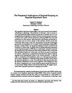
Figure 1: The relation between a credible set and its associated confidence set in terms of Venn diagrams: the extra points θ in the associated confidence set C not included in the credible set D are characterized by non-empty intersection B(θ) ∩ D 6= ∅. Corollary 4.15 For all n ≥ 1, assume that (X1 , X2 , . . . , Xn ) ∈ X n ∼ P0n for some P0 ∈ P. Let Πn denote Borel priors on P, with constant C > 0 and rate sequence n ↓ 0 such that (13) is satisfied for all θ0 ∈ Θ. Denote by Dn credible sets of level 1 − exp(−C 0 n2n ), for some C 0 > C. Then the minimal confidence sets Cn associated with Dn under radius-n Hellinger-enlargement are asymptotically consistent. Note that in the above corollary, diamH (Cn (X n )) = diamH (Dn (X n )) + n , almost surely. If, in addition to the conditions in the above corollary, tests satisfying (12) with an = exp(−C 0 n2n ) exist, the posterior is consistent at rate n and sets Dn (X n ) have diameters decreasing as n (although they can be non-spherical). In the case n is the optimal rate of convergence for the problem, the confidence sets Cn (X n ) attain optimallity in the sense that their sizes decrease at the optimal rate. In order for this statement to allow an assertion that involves a specific confidence level (rather than just resulting in asymptotic coverage), we may specify the definition of remote contiguity slightly further. Definition 4.16 Given measurable spaces ((Xn , Bn ) : n ≥ 1) with two sequences (Pn ) and (Qn ) of probability measures and sequences ρn , σn , ρn , σn > 0, ρn , σn → 0, we say 19

that Qn is ρn -to-σn remotely contiguous with respect to Pn , notation σn−1 Qn C ρ−1 n Pn , if, Pn φn (X n ) = o(ρn )

⇒

Qn φn (X n ) = o(σn ).

for every sequence of Bn -measurable φn : Xn → [0, 1]. Like definition 3.1, definition 4.16 allows for re-formulation similar to lemma 3.3, e.g. if for some sequence cn ,

Qn − Qn ∧ cn a−1

n Pn = o(cn ), −1 then c−1 n Qn C an Pn . We leave the formulation of other sufficient conditions to the

reader. If we re-write the last condition of theorem 4.14 as follows Π |Bn (θ0 )

n −1 (ii’) c−1 n Pθ0 ,n C bn an Pn

.

the last step in the proof of theorem 4.14 is more specific; particularly, assertion (15) becomes,
Pθ0 ,n θ ∈ Dn (X n ) = o(cn ), i.e. the confidence level of the sets Dn (X n ) is 1 − Kcn asymptotically (for some constant K > 0 and large enough n).

5

Discussion

The conclusion of this paper is that there exists a systematic way of taking a Bayesian limit into a frequentist one, if the prior satisfies an extra condition relating the true data distributions to suitable local prior predictive distributions. Doob shows that a Bayesian form of posterior consistency with i.i.d. samples obtains without any real conditions on the model. But to the frequentist, ‘holes’ of inconsistency remain: there exists a prior null-set of distributions for the data that do not lead to convergent posteriors, or to convergence at a false point in the model. The extra condition ‘fixes these holes’ and extends the Bayesian form of consistency to the frequentist notion. The existence of a Bayesian test sequence (which is equivalent to prior-almostsure posterior consistency, c.f. theorem 2.6) is extended to posterior consistency in the frequentist sense with said condition, and Bayesian credible sets are extended to serve as confidence sets. In both extensions, upper bounds on testing power and credible/confidence level are balanced directly with lower bounds on prior probability present ‘locally’ around the true value of the parameter. Since Freedman’s counterexamples and Schwartz’s proof it has been apparent that such balancing is of the essence when using posteriors in frequentist asymptotics. Remote contiguity makes room for the matching of rates between upper and lower bounds and gives meaning to the notion of locality above. 20

Comparing contiguity with its remote variant, two related examples in regression characterize the difference perhaps most clearly: we concentrate on samples X n of pairs (X, Y ) ∈ R2 assumed related through Y = f0 (X) + e for some unknown f0 ∈ F , with i.i.d. standard normal errors independent of i.i.d. covariates with distribution P . It is assumed that F ⊂ L2 (P ) and, given an f ∈ F , we denote the sample distributions as Pf,n . We distinguish two cases: (a) the parametric case of linear regression, where F = {fθ : R → R : θ ∈ Θ}, with θ = (a, b) ∈ Θ = R2 and fθ (x) = ax + b; and (b) the case of non-parametric regression, where we do not restrict F beforehand. In examples D.16 and D.17, remote contiguity is compared to contiguity. Following lemmas 3.3 and B.2, both properties are analysed through local averages of the likelihood 1

2

process. In the non-parametric case with an = e 2 nτ , the an -re-scaled likelihood process is written as, a−1 n

1 Pn 2 2 dPf,n (X n ) = e− 2 i=1 (ei (f −f0 )(Xi )+(f −f0 ) (Xi )−τ ) dPf0 ,n

(16)

under Pf0 ,n . In the parametric case, where the parameter is θ = (a, b) ∈ Θ = R2 , the likelihood takes the familiar LAN form: for h ∈ R2 and θn = θ0 + hn−1/2 , Pn dPθn ,n n √1 h·` (X ,Y )− 1 h·I ·h+oPθ ,n (1) 0 , (X ) = e n i=1 θ0 i i 2 θ0 dPθ0 ,n

where `θ0 is the score function for θ and Iθ0 is the Fisher information. Proofs for (remote) contiguity in the parametric and non-parametric cases now proceed quite differently. In Pθ0 ,n -w. P −−→ N2 (0, Iθ0 ) ultimately the parametric case, the central limit n−1/2 i `θ0 (Xi , Yi ) −−− implies contiguity of local prior predictive distributions for priors of full support and testing power only plays a role to lower bound prior mass in n−1/2 neighbourhoods of θ0 . In the non-parametric case, the argument is more crude: the law of large numbers establishes that the n−1 times the exponent of (16) converges to − 12 (kf − f0 k2P,2 − τ 2 ), which suffices for a proof of remote contiguity assuming a prior on L2 (P ) that includes F in its support. Clearly a proof of contiguity puts requirements on the likelihood of a relatively stringent nature compared to the requirements posed by remote contiguity. The LAN example relies on quite subtle argumentation that is natural in parametric context, but cannot be expected to generalize to the same powerful extent in non-parametric setting (notwithstanding successes in semi-parametric statistics). In non-parametric cases, a less delicate argument is required and remote contiguity appears to provide this, as supported by application to Bayesian non-parametric questions in this paper. From that perspective it is conceivable that the remote variant of contiguity can fulfill a much wider role in non-parametric statistics. Future efforts will focus on several areas of research: first of all, more non-parametric applications must be analysed. Here and there in the main text are some ambitious 21

suggestions (with answers that would be too lengthy to include). Of primary interest are challenging cases that could not be dealt with in a systematic way before: parameter spaces that grow with the sample size, data that does not adhere to the i.i.d. sampling scheme, parameter spaces without an obvious default choice for the prior. Possible applications include an analysis of the requirement on priors for sparse sequence models (like the horseshoe), testing/classification of hypotheses on models in which the parameter or the observation is a graph, models for highly dependent data and stochastic processes and weak consistency with process priors. Of special interest are statistical questions that involve more than consistent point-estimation, like model selection and the coverage of credible sets. More generally, all examples of ways to satisfy the conditions of lemma 3.3 are of interest. Secondly, it appears interesting to find creative ways to formulate and apply remote contiguity. Like contiguity, remote contiguity provides a way to approximate limit behaviour of statistics under alternatives: given that Qn C a−1 n Pn , prove that Pn (An ) = o(an ) in the approximation and conclude Qn (An ) = o(1) under the truth. Of particular interest may be an extension of remote contiguity with an assertion that is uniform over a subset F of Θ, sup Qθ,n C a−1 n Pn , θ∈F

for which it is sufficient that, for some constant c > 0, sup kQθ,n − Qθ,n ∧ ca−1 n Pn k → 0. θ∈F

with obvious uniform reformulations of other sufficient conditions. As pointed out by Le Cam in chapter 6 of [34], the above is closely related to weak compactness in T∞ and the famous Dunford-Pettis theorem. Uniform domination of probabilities over subsets of the model make possible many constructions, involving finite approximations, minimax efficiency and the study of distributions under alternatives (like the property of regularity of an estimator sequence in parametric setting). In this context it may be of interest that there exists a version of the convolution theorem that does not require regularity of the estimator but leaves room for exceptions on a subset of Lebesgue measure zero.

A

Definitions and conventions

Because we take the perspective of a frequentist using Bayesian methods, we are obliged to demonstrate that Bayesian definitions continue to make sense under the assumptions that the data X is distributed according to a true, underlying P0 . Remark A.1 We assume given for every n ≥ 1, a measurable (sample) space (Xn , Bn ) and random sample X n ∈ Xn , with a model Pn of probability distributions Pn : Bn → 22

[0, 1]. It is also assumed that there exists an n-independent parameter space Θ with a Hausdorff, completely regular topology T and associated Borel σ-algebra G , and, for every n ≥ 1, a bijective model parametrization Θ → Pn : θ 7→ Pθ,n , that is such that for every n ≥ 1 and every A ∈ Bn , the map Θ → [0, 1] : θ 7→ Pθ,n (A) is measurable. Any prior Π on Θ is assumed to be a Borel probability measure Π : G → [0, 1] and can vary with the sample-size n. As frequentists, we assume that there exists a “true, underlying distribution for the data”; in this case, that means that for every n ≥ 1, there exists a distribution P0,n that describes the distribution of the n-th sample X n .



Often one assumes, in addition, that the model is well-specified : that there exists a θ0 ∈ Θ such that P0,n = Pθ0 ,n for all n ≥ 1. We think of Θ as a topological space because we want to discuss estimation as a procedure of sequential, stochastic approximation of and convergence to such a “true parameter value” θ0 . Additionally we sometimes make the technical assumption that the observations X n are coupled, in the sense that all X n , n ≥ 1 can be realized as a stochastic process, i.e. simultaneously as random variables X n : Ω → Xn on a probability space (Ω, F , P¯0 ) such that P¯0 (X n−1 (A)) = P0,n (X n ∈ A) for all n ≥ 1 and A ∈ Bn . For example, in the case of i.i.d. data, a coupling exists: we take Ω = X ∞ with the σ-algebra generated by the cylinder sets and the product distribution P¯0 = P ∞ . In cases where the X n describe more complicated, dependent 0

data like time-series, finite-dimensional marginals that are consistent in Kolmogorov’s sense give rise to a coupling. In most of this paper, coupling is not required; in places where it is, coupling is mentioned explicitly. Definition A.2 Given n, m ≥ 1 and a prior probability measure Πn : G → [0, 1], define the n-th prior predictive distribution on Xm as follows: Z Πn Pθ,m (A) dΠn (θ), Pm (A) =

(17)

Θ

for all A ∈ Bm . If the prior is replaced by the posterior, the above defines the n-th posterior predictive distribution on Xm , Z Πn |X n Pm (A) = Pθ,m (A) dΠn (θ|X n ),

(18)

Θ

for all A ∈ Bm . For any Bn ∈ G with Πn (Bn ) > 0, define also the n-th local prior predictive distribution on Xm , Πn |Bn Pm (A) =

1 Πn (Bn )

Z Pθ,m (A) dΠn (θ),

(19)

Bn

as the predictive distribution on Xm that results from the prior Πn when conditioned on Bn . If m is not mentioned explicitly, it is assumed equal to n. The prior predictive distribution PnΠn is the marginal distribution for X n in the Bayesian perspective that considers parameter and sample jointly (θ, X n ) ∈ Θ×Xn as the random quantity of interest. 23

Definition A.3 Given n ≥ 1, a (version of) the posterior is any map Πn ( · |X n = · ) : G × Xn → [0, 1] such that, (i.) for any B ∈ G , the map Xn → [0, 1] : xn 7→ Πn (B|X n = xn ) is Bn -measurable; (ii.) for all A ∈ Bn and V ∈ G , Z Z n Πn Pθ,n (A) dΠn (θ). Πn (V |X ) dPn =

(20)

V

A

Bayes’s Rule is expressed through equality (20) and is sometimes referred to as a ‘disintegration’ (of the joint distribution of (θ, X n )). If the posterior is a Markov kernel, it is a PnΠn -almost-surely well-defined probability measure on (Θ, G ). But it does not follow from the definition above that a version of the posterior actually exists as a regular conditional probability measure. Under mild, extra conditions, regularity of the posterior can be guaranteed: for example, if samplespace and parameter space are Polish, the posterior is regular; if the model Pn is dominated (denote the density of Pθ,n by pθ,n ), the fraction of integrated likelihoods, Z Z Πn (V |X n ) = pθ,n (X n ) dΠn (θ) pθ,n (X n ) dΠn (θ), V

(21)

Θ

for V ∈ G , n ≥ 1 defines a regular version of the posterior distribution. Remark A.4 As a consequence of the frequentist assumption that X n ∼ P0,n for all n ≥ 1, the PnΠn -almost-sure definition (20) of the posterior Πn (V |X n ) does not make sense automatically (see Freedman (1963) [16], Kleijn and Zhao (2016) [27]): null-sets of PnΠn on which the definition of Πn ( · |X n ) is ill-determined, may not be null-sets of P0,n . To prevent this, we impose the domination condition, P0,n  PnΠn .

(22)

for every n ≥ 1.



To understand the reason for (22) in a perhaps more familiar way, consider a dominated model and assume that for certain n, (22) is not satisfied. Then, using (17), we find,  Z P0,n pθ,n (X n ) dΠn (θ) = 0 > 0, so the denominator in (21) evaluates to zero with non-zero P0,n -probability. To get an idea of sufficient conditions for (22), it is noted in [27] that in the case of i.i.d. data where P0,n = P0n for some marginal distribution P0 , P0n  PnΠ for all n ≥ 1, if P0 lies in the Hellinger- or Kullback-Leibler-support of the prior Π. For the generalization to the present setting we are more precise and weaken the topology appropriately. (See appendix C and remark 3.6 (2) in Strasser (1985) [42].) Proposition A.5 Given n ≥ 1, if P0,n lies in the Tn -support of Πn , then P0,n  PnΠn . 24

Notation and conventions Non-standard abbreviations: s.t. stands for “such that”; f.l.e.n. stands for “for large enough n”; l.h.s. and r.h.s. refer to “left-” and “right-hand sides” respectively. For given probability measures P, Q on (X , B) and a σ-finite measure µ that dominates both (e.g. µ = P + Q), denote dP/dµ = p and dQ/dµ = q. For the likelihood ratio dQ/dP (which concerns only the P -dominated component of Q, following [34]), note that the measurable map q/p 1{p > 0, q > 0} : X → R is a µ-almost-everywhere version of dQ/dP . Given a probability space (Ω, F , P ), a measurable map X : Ω → R is called a random variable if X is tight (i.e. if P (|X| < ∞) = 1). The integral of a real-valued, integrable random variable X with respect to a probability measure P is often denoted P X, while integrals over the model with respect to priors and posteriors are always written out in Leibniz’s notation. Given  > 0 and a metric space (Θ, d), the covering number N (, Θ, d) ∈ N ∪ {∞} is the minimal cardinal of a cover of Θ by d-balls of radius . Given real-valued random variables X1 , . . . , Xn , the first order statistic is X(1) = min1≤i≤n Xi . The total-variational norm and Hellinger distance are denoted k · k and H(·, ·), respectively. The Hellinger diameter of a model subset C is denoted diamH (C)

B

Contiguity

First, let us recall the definition of contiguity [31] (see [34] for alternatives, e.g. in terms of limiting domination in a sequence of binary experiments.) Definition B.1 Given measurable spaces (Xn , Bn ), n ≥ 1 with two sequences (Pn ) and (Qn ) of probability measures, we say that Qn is contiguous with respect to Pn , notation Qn C Pn , if, Pn φn (X n ) = o(1)

⇒

Qn φn (X n ) = o(1).

(23)

for every sequence of Bn -measurable φn : Xn → [0, 1]. The value of the notion of contiguity does not just reside with the usefulness of the property itself, but also with the multitude of accessible characterizations listed in Le Cam’s ˘ ak (1967) [24]). (One of the formulations famous First Lemma (see, e.g., Haj´ek and Sid´ R requires that we define the so-called Hellinger transform ψ(P, Q; α) = pα q 1−α dµ, where p and q denote densities for P and Q with respect to a σ-finite measure that dominates both Pn and Qn .) Lemma B.2 (Le Cam’s First Lemma) Given measurable spaces ((Xn , Bn ) : n ≥ 1) with two sequences (Pn ) and (Qn ) of probability measures, the following are equivalent:

25

(i) Qn C Pn ; P

Qn

n (ii) For any measurable Tn : Xn → R, if Tn −−→ 0, then Tn −−→ 0;

(iii) Given  > 0, there is a b > 0 such that Qn (dQn /dPn > b) < , f.l.e.n.; (iv) Given  > 0, there is a c > 0 such that kQn − Qn ∧ c Pn k < , f.l.e.n.; Qn -w.

(v) If dPn /dQn −−−−→ f along a subsequence, then P (f > 0) = 1; P -w.

(vi) If dQn /dPn −−n−−→ g along a subsequence, then Eg = 1; (vii) Hellinger transforms satisfy, lim inf n limα↑1 ψ(Pn , Qn ; α) = 1. A proof of this form of the First Lemma can be found in [34], section 6.3. Note the relation to testing: for two sequences (Pn ), (Qn ) that are mutually contiguous (Pn C Qn and Qn C Pn ), there exists no test sequence that separates (Pn ) from (Qn ) asymptotically. Loosely said, (Pn ) and (Qn ) are indistinguishable statistically regardless of the amount of data available. Much more can be said about contiguity (to begin with, see, Roussas (1972) [38] and Greenwood and Shiryaev (1985) [23]), for instance in relation to Le Cam’s convergence of experiments, but also, specific relations that exist in the locally asymptotically normal case (e.g. Le Cam’s Third lemma [24], which relates the laws of a statistic under Pn and Qn in such context).

C

Weak model topologies

Throughout this text weak model topologies are used. Below we provide definitions, some intriguing properties and relations with more commonly used (metric) topologies. Definition C.1 Given a measurable space (X , B) and a model P for observation of a random variable X ∈ X . Let F denote a class of bounded, measurable functions f : X → R. The weak topology TF on P is the weakest topology on P such that for every f ∈ F , the map P 7→ P f is continuous. For P ∈ P, f ∈ F , 0 ≤ f ≤ 1 and  > 0, the sets WP,f, = {Q ∈ P : |(P − Q)f | < }, form a fundamental system of neighbourhoods on P for the weak topology TF . Example C.2 For all n ≥ 1, Tn denotes the weak topology on Pn corresponding to the class Fn of all bounded, Bn -measurable f : Xn → R.



Example C.3 If we model single-observation distributions P ∈ P for an i.i.d. sample, the topology Tn on Pn = P n induces a topology on P (which we also denote by Tn ) for each n ≥ 1. The union T∞ = ∪n Tn forms a topology that allows formulation of conditions for the existence of consistent estimates that are not only sufficient, but also necessary (see Le Cam and Schwartz (1960) [30]), offering a precise perspective on what is estimable and what is not in i.i.d. context. 26



Example C.4 For Hausdorff completely regular sample spaces X , Prokhorov’s weak topology TC is defined as the weak topology generated by the family FC of all bounded, continuous functions X → R. According to Prokhorov’s theorem, compactness in this topology corresponds to uniform tightness. The portmanteau lemma provides equivalent characterizations. Definition C.5 The strong topology β on P associated with F has a fundamental system of neighbourhoods of the form,  B(P, ) = Q ∈ P : sup{|(P − Q)f | : f ∈ F, 0 ≤ f ≤ 1} <  for P ∈ P and  > 0. A so-called polar topology is a topology on P between weak and strong: P → Q in a polar topology, when |P f − Qf | goes to zero, uniformly over any G ⊂ F of a certain type, e.g. any compact G in F . Example C.6 In the case of Tn , the associated strong topology on Pn is the totalvariational topology. If we model an i.i.d. sample, the strong topologies associated with all Tn and T∞ are equal (to the usual total-variational metric topology on P = P1 ). For more on these topologies, the reader is referred to Strasser (1985) [42] and to Le Cam (1986) [34].

D D.1

Applications and examples Inconsistent posteriors

Calculations that demonstrate instances of posterior inconsistency are many (for a nonexhaustive list of examples, see, [10, 11, 8, 12, 13, 18, 19]). In this subsection, we illustrate some of these examples of posterior inconsistency that illustrate the problem clearly, without too many distracting technicalities. Example D.1 (Freedman (1963) [16]) Consider a sample X1 , X2 , . . . of random positive integers. Denote the space of all probability distributions on N by Λ and assume that the sample is i.i.d.-P0 , for some P0 ∈ Λ. For any P ∈ Λ, write p(i) = P ({X = i}) for all i ≥ 1. The total-variational and weak topologies on Λ are equivalent (defined, P → Q if p(i) → q(i) for all i ≥ 1). Let Q ∈ Λ \ {P0 } be given. To arrive at a prior with P0 in its support, leading to a posterior that concentrates on Q, we consider sequences (Pm ) and (Qn ) such that Qm → Q and Pm → P0 as m → ∞. The prior Π places masses αm > 0 at Pm and βm > 0 at Qm (m ≥ 1), so that P0 lies in the support of Π. A careful construction of the distributions

27

Qm that involves P0 , guarantees that the posterior satisfies, Πn ({Qm }|X n ) P0 -a.s. −−−−→ 0, Πn ({Qm+1 }|X n ) that is, posterior mass is shifted further out into the tail as n grows to infinity, forcing all posterior mass that resides in {Qm : m ≥ 1} into arbitrarily small neighbourhoods of Q. In a second step, the distributions Pm and prior weights αm are chosen such that the posterior mass in {Pm : m ≥ 1} becomes negligible with respect to the posterior mass in {Qm : m ≥ 1}. Like the Qm , the Pm are chosen such that likelihood at various Pm grows large for high values of m and small for lower values with increasing n. Consequently, the posterior mass in {Pm : m ≥ 1} also accumulates in the tail. However, the prior weights αm may be chosen to decrease very fast with m, in such a way that, Πn ({Pm : m ≥ 1}|X n ) P0 -a.s. −−−−→ 0, Πn ({Qm : m ≥ 1}|X n ) thus forcing all posterior mass into {Qm : m ≥ 1} as n grows. This leads to the conclusion that for every neighbourhood UQ of Q, P -a.s.

Πn (UQ |X n ) −−0−−→ 1, so the posterior is inconsistent. Other choices of the weights αm that place more prior mass in the tail do lead to consistent posterior distributions.



One may object to Freedman’s construction, in that knowledge of P0 is required to choose the prior that causes inconsistency. To strengthen Freedman’s point one would need to construct a prior of full support without explicit knowledge of P0 . Example D.2 (Freedman (1965) [17]) In the setting of example D.1, denote the space of all distributions on Λ by π(Λ). Note that since Λ is Polish, so is π(Λ) and so is the product Λ × π(Λ). Freedman’s theorem says that the set of pairs (P0 , Π) ∈ Λ×π(Λ) such that for all open U , P0n Π(U |X n ) goes to one along a subsequence is residual. Consequently, the set of pairs (P0 , Π) ∈ Λ×π(Λ) for which the posterior is consistent is meagre in Λ × π(Λ). The proof relies on the following construction: for k ≥ 1, define Λk to be the subset of all probability distributions P on N such that P (X = k) = 0. Also define Λ0 as the union of all Λk , (k ≥ 1). Pick Q ∈ Λ \ Λ0 . We assume that P0 ∈ Λ \ Λ0 and P0 6= Q. Place a prior Π0 on Λ0 and choose Π = 21 Π0 + 12 δQ . Because Λ0 is dense in Λ, priors of this type have full support in Λ. But P0 has full support in N so for every k ∈ N, P0∞ (∃m≥1 : Xm = k) = 1: note that if we observe Xm = k, the likelihood equals zero on Λk so that Πn (Λk |X n ) = 0 for all n ≥ m, P0∞ -almost-surely. Freedman shows this eliminates all of Λ0 asymptotically, if Π0 is chosen in a suitable way, forcing all posterior mass onto the point {Q}. (See also, Le Cam (1986) [34], section 17.7).

 28

The question remains how Freedman’s inconsistent posteriors relate to the work presented here. Since test sequences of exponential power exist to separate complements of weak neighbouthoods, c.f. proposition 2.4, Freedman’s inconsistencies must violate the requirement of remote contiguity in theorem 4.4. Example D.3 The `1 -subspace Λ of all probability measures on N is a Polish space. In particular, Λ is metric and second countable so Λ \ Λ0 contains a countable dense subset D. For Q ∈ D, let V be the set of all prior probability measures on Λ with finite support, of which one point is Q and the remaining points lie in Λ0 . The proof of the theorem in [17] that asserts that the set of consistent pairs (P0 , Π) is of the first category in Λ × π(Λ) departs from the observation that if P0 lies in Λ \ Λ0 and we use a prior from V , then, P -a.s.

Π({Q}|X n ) −−0−−→ 1, (in fact, as is shown below, with P0∞ -probability one there exists an N ≥ 1 such that Π({Q}|X n ) = 1 for all n ≥ N ). The proof continues to assert that V lies dense in π(Λ), and, through sequences of continuous extensions involving D, that posterior inconsistency for elements of V implies posterior inconsistency for all Π in π(Λ) with the possible exception of a set of the first category. From the present perspective it is interesting to view the inconsistency of elements of V in light of the conditions of theorem 4.4. Define, for some bounded f : N → R and  > 0, B = {P ∈ Λ : |P f − P0 f | < 21 },

V = {P ∈ Λ : |P f − P0 f | ≥ }.

Proposition 2.4 asserts the existence of a uniform test sequence for B versus V of exponential power. With regard to remote contiguity, for an element Π of V with support of order M + 1, write, Π = βδQ +

M X

α m δ Pm ,

m=1

where β +

P

m αm

= 1 and Pm ∈ Λ0 (1 ≤ m ≤ M ). Without loss of generality, assume

that  and f are such that Q does not lie in B. Consider Π|B

dPn 1 (X n ) = n dP0 Π(B)

Z B

M n dP n n 1 X dPm (X ) dΠ(P ) ≤ α (X n ). m dP0n Π(B) dP0n m=1

For every 1 ≤ m ≤ M , there exists a k(m) such that Pm (X = k(m)) = 0, and the probability of the event En that none of the X1 , . . . , Xn equal k(m) is (1 − P0 (X = n /dP n (X n ) > 0. k(m)))n . Note that En is also the event that dPm 0

Hence for every 1 ≤ m ≤ M and all X in an event of P0∞ -probability one, there exists n /dP n (X n ) = 0 for all n ≥ N . Consequently, for all X in an Nm ≥ 1 such that dPm m 0 Π|B

an event of P0∞ -probability one, there exists an N ≥ 1 such that dPn

29

/dP0n (X n ) = 0

for all n ≥ N . Therefore, condition (ii) of lemma 3.3 is not satisfied for any sequence an ↓ 0. A direct proof is also possible: given the prior Π ∈ V , define, φn (X n ) =

M Y

1{∃1≤i≤n :Xi =k(m)}

m=1

Then the expectation of φn with respect to the local prior predictive distribution equals Π|B

zero, so Pn

φn = o(an ) for any an ↓ 0. However, P0n φn (X n ) → 1, so the prior Π does Π|B

not give rise to a sequence of prior predictive distributions (Pn (P0n )

D.2

) with respect to which

is remotely contiguous, for any an ↓ 0.



Frequentist estimation with posteriors

Proofs concerning posterior consistency or posterior convergence at a rate often require the existence of exponentially powerful Bayesian or uniform tests for small parameter subsets Bn surrounding a point θ0 ∈ Θ, versus the complements Vn of neighbourhoods of the point θ0 . Although the sets Bn can often be chosen to be convex, complements of neighbourhoods are typically non-convex. Imposing Hellinger pre-compactness (or, in the case of rates, bounds on the Hellinger entropy) offers a way to achieve this, with the use of proposition 2.5. Example D.4 Consider a model P of distributions P for i.i.d. data (X1 , X2 , . . . , Xn ) ∼ P n , (n ≥ 1) and, in addition, suppose that P is totally bounded with respect to the Hellinger distance. Let P0 ∈ P and  > 0 be given, denote V () = {P ∈ P : H(P0 , P ) ≥ 4}, BH () = {P ∈ P : H(P0 , P ) < }. There exists an N () ≥ 1 and a cover of V () by H-balls V1 , . . . , VN () of radius  and for any point Q in any Vi and any P ∈ BH (), H(Q, P ) > 2. According to proposition 2.5, for each 1 ≤ i ≤ N () there exists a uniform test sequence (φi,n ) for BH () versus Vi of power exp(−2n2 ). Defining for all n ≥ 1, φn = max{φi,n : 1 ≤ i ≤ N ()}, we obtain a test sequence such that, sup P ∈BH ()

2

P n φn + sup P n φn ≤ (N () + 1) e−2n ≤ e−n

2

(24)

Q∈V ()

for large enough n. If  = n with n ↓ 0 and n2n → ∞, and the model’s Hellinger entropy is upper-bounded by log N (n , P, H) ≤ Kn2n for some K > 0, the construction extends to tests that separate Vn = {P ∈ P : H(P0 , P ) ≥ 4n } from Bn = {P ∈ P : H(P0 , P ) < n } asymptotically, with power exp(−nL2 ) for some L > 0. (For more on this construction (including the so-called Le Cam dimension of a model), see Le Cam (1973) [32] and the rate-oriented work in Birg´e (1983,1984) [4, 5].)



The uniform tests of example D.4 require pre-compactness of the model in the Hellinger topology, which, although customary in many settings, is quite a strong requirement. Barron (1988) [1] and Barron et al. (1999) [2] formulate a requirement based on the Radon property that any prior on a Polish space has. 30

Example D.5 Consider a model P of distributions P for i.i.d. data (X1 , X2 , . . . , Xn ) ∼ P n , (n ≥ 1), with priors (Πn ). Assume that the model P is Polish in the Hellinger topology. Let P0 and  > 0 be given; for a fixed M > 1, define V () = {P ∈ P : H(P0 , P ) ≥ M }, BH () = {P ∈ P : H(P0 , P ) < }. For any sequence δm ↓ 0, there exist compacta Km ⊂ P for all m ≥ 1 such that Π(Km ) ≥ 1 − δm . For each m ≥ 1, Km is Hellinger totally bounded so there exists a uniform test sequence φm,n for BH () ∩ Km versus V () ∩ Km . Since, Z Z Qn (1 − φn ) dΠ(Q) P n φn dΠ(P ) + V () BH () Z Z n ≤ P φm,n dΠ(P ) + Qn (1 − φm,n ) dΠ(Q) + δm BH ()∩Km

V ()∩Km

and all three terms go to zero, a diagonalization argument confirms the existence of a Bayesian test. To control the power of this test and to generalize to the case where  = n is n-dependent, more is required: as we increase m with n, the prior mass δm(n) outside of Kn = Km(n) must drop of fast enough, while the order of the cover must be bounded: if Πn (Kn ) ≥ 1 − exp(−L1 n2n ) and the Hellinger entropy of Kn satisfies log N (n , Kn , H) ≤ L2 n2n for some L1 , L2 > 0, there exist M > 1, L > 0, and a sequence of tests (φn ) such that, Z Z P n φn dΠ(P ) + BH (n )

2

Qn (1 − φn ) dΠ(Q) ≤ e−Lnn ,

V (n )

for large enough n. (For related constructions, see Barron (1988) [1], Barron et al. (1999) [2] and Ghosal, Ghosh and van der Vaart (2000) [21].) To apply corollary 4.5 consider the following steps. Example D.6 As an example of the tests required under condition (i) of corollary 4.5, consider P in the Hellinger topology, assuming totally-boundedness. Let U be the Hellinger-ball of radius 4 around Pθ0 of example D.4 and let V be its complement. The Hellinger ball BH () in equation 24 contains the set K(), so the test sequence for BH () versus V is also a test for K() versus V , of the same power. Alternatively we may consider the model in any of the weak topologies Tn : let  > 0 be given and let U denote a weak neighbourhood of the form {P ∈ P : |(P n − P0n )f | ≥ 2}, for some bounded measurable f : Xn → [0, 1], as in proposition 2.4. The set B of proposition 2.4 contains a set K(δ), for some δ > 0. Both these applications were noted by Schwartz in [40]. To appreciate the relevance of priors satisfying the lower bound (13), let us repeat lemma 8.1 in [21], to demonstrate that the sequence (P0n ) is with respect to the local prior predictive distributions based on the Bn of example 4.8. Lemma D.7 For all n ≥ 1, assume that (X1 , X2 , . . . , Xn ) ∈ X n ∼ P0n for some P0 ∈ P and let n ↓ 0 be given. Let Bn be as in example 4.8. Then, for any priors Πn such that 31

Πn (Bn ) > 0, Z Pθ0 ,n

dPθn 2 (X n ) dΠn (θ|Bn ) < e−cnn dPθn0

 → 0,

for any constant c > 1.

D.3

Consistency without KL priors

Below it is demonstrated that example 1.4, which does not admit KL priors, satisfies the requirement of remote contiguity. We start by showing that remote contiguity obtains (choose η equal to the uniform density for simplicity). Example D.8 Consider X1 , X2 , . . . that form an i.i.d. sample from the uniform distribution on [θ, θ+1], for unknown θ ∈ R. The model is parametrized in terms of distributions Pθ with Lebesgue densities of the form pθ (x) = 1[θ,θ+1] (x), for θ ∈ Θ = R. Pick a prior Π on Θ with a continuous and strictly positive Lebesgue density π : R → R and, for some rate δn ↓ 0, choose Bn = (θ0 , θ0 + δn ). Note that for any α > 0, there exists an N ≥ 1 such that for all n ≥ N , (1 − α)π(θ0 )δn ≤ Π(Bn ) ≤ (1 + α)π(θ0 )δn . Note that for any θ ∈ Bn and X n ∼ Pθn0 , dPθn /dPθn0 (X n ) = 1{X(1) > θ}, and correspondingly, Π|B

dPn n n (X ) = Πn (Bn )−1 dPθn0

θ0 +δn

Z

1{X(1) > θ} dΠ(θ) ≥ θ0

1 − α δn ∧ (X(1) − θ0 ) 1+α δn

for large enough n. As a consequence, for every δ > 0 and all an ↓ 0, Z 
dPθ,n n n Pθ0 (X ) dΠn (θ|Bn ) < δ an ≤ Pθn0 δn−1 (X(1) − θ0 ) < (1 + α)δ an dPθ0 ,n for large enough n ≥ 1. Since n(X(1) − θ0 ) has an exponential weak limit under Pθn0 , we choose δn = n−1 , so that the r.h.s. in the above display goes to zero. So Pθ0 ,n C Π |Bn

n a−1 n Pn

, for any an ↓ 0



To show consistency and derive the posterior rate of convergence in example 1.4, we use theorem 4.6. Example D.9 Continuing with example D.8, we define Vn = {θ : θ − θ0 > n }. It is noted that, for every 0 < c < 1, the likelihood ratio test, φn (X1 , . . . , Xn ) = 1{dPθ0 +n ,n /dPθ0 ,n (X n ) > c} = 1{X(1) > θ0 + n }, satisfies Pθn (1 − φn )(X n ) = 0 for all θ ∈ Vn , and if we choose δn = 1/2 and n = Mn /n for some Mn → ∞, Pθn φn ≤ e−Mn +1 for all θ ∈ Bn , so that, Z Z n n Pθ φn (X ) dΠ(θ) + Pθn (1 − φn (X n )) dΠ(θ) ≤ Π(Bn ) e−Mn +1 , Bn

Vn Π|Bn

Using lemma 2.2, we see that Pn

Π(Vn |X n ) ≤ e−Mn +1 . Based on the conclusion of

example D.8 above, remote contiguity implies that Pθn0 Π(Vn |X n ) → 0. Treating the case 32

θ < θ0 − n similarly, we conlude that the posterior is consistent at (any n slower than) rate 1/n.

D.4

Finite sample spaces and the tailfree case

Example D.10 Consider the situation where we observe an i.i.d. sample of random variables X1 , X2 , . . . taking values in a space X of finite order N . Writing X as the set of integers {1, . . . , N }, we note that the space M of all probability measures P on (X , 2X ) with the total-variational metric (P, Q) 7→ kP − Qk is in isometric correspondence with the simplex,  SN = p = (p(1), . . . , p(N )) ∈ [0, 1]N : p(k) ≥ 0, (1 ≤ k ≤ N ), Σi p(i) = 1 , with the metric (p, q) 7→ kp−qk = Σk |p(k)−q(k)| it inherits from RN with the L1 -norm, when k 7→ p(k) is the density of P ∈ M with respect to the counting measure. We also define RN = {p ∈ SN : p(k) > 0, 1 ≤ k ≤ N } and M 0 = {P ∈ M : P ({k}) > 0, 1 ≤ k ≤ N }. Proposition D.11 If the data is an i.i.d. sample of X -valued random variables and X is of finite order, then for any n ≥ 1, any Borel prior Π : G → [0, 1] of full support on M , any P0 ∈ M and any ball B around P0 , there exists an 0 > 0 such that, 1

2

P0n C e 2 n PnΠ|B ,

(25)

for all 0 <  < 0 . Proof By the inequality kP − Qk ≤ −P log(dQ/dP ), the ball B around P0 contains a set of the form K() = {P ∈ M 0 : −P0 log(dP/dP0 ) < δ}, and because the mapping P 7→ −P0 log(dP/dP0 ) is continuous on M 0 , there exists an open neighbourhood B 0 of P0 in M such that B 0 ∩ M 0 ⊂ K(). Since both M 0 and B 0 are open and Π has full support, Π(K()) ≥ Π(B 0 ∩ M 0 ) > 0. With the help of example 3.2, we see that for every P ∈ K(),

dP n n (X ) ≥ 1, dP0n for large enough n, P0 -almost-surely. Fatou’s lemma then says that, Z 1 2 dP n n n 2 lim inf e (X ) dΠ(θ|K()) ≥ 1, n→∞ dP0n 1

e 2 n

2

with P0∞ -probability one, so condition (ii) of lemma 3.3 is satisfied. Conclude that assertion (25) holds.



Example D.12 We continue with the situation where we observe an i.i.d. sample of random variables X1 , X2 , . . . taking values in a space X of finite order N . For given  > 0, consider the hypotheses, B = {P ∈ M : kP − P0 k < },

V = {Q ∈ M : kQ − P0 k > 2}. 33

Noting that M is compact (or with the help of the simplex representation SN ) one sees that entropy numbers of M are bounded, so the construction of example D.4 shows that uniform tests of exponential power e−nD (for some D > 0) exist for B versus V . Application of proposition D.11 shows that the choice of an 0 > 0 small enough guarantees that Πn (V |X n ) goes to zero in P0n -probability. Conclude that the posterior resulting from a prior Π of full support on M is consistent in total variation. Example D.13 With geberal reference to Ferguson (1973) [15], one way to construct non-parametric priors concerns a refining sequence of finite, Borel measurable partitions of a sample space, say X = R: to define a ‘random distribution’ P on R, we specify for each such partition α = {A1 , . . . , AN }, a Borel prior Πα on SN , identifying (p1 , . . . , pN ) with the ‘random variables’ (P (A1 ), . . . , P (AN )). Kolmogorov existence of the stochastic process describing all P (A) in a coupled way subjects these Πα to consistency requirements expressing that if A1 , A2 partition A, then P (A1 ) + P (A2 ) must have the same distribution as P (A). If the partitions refine appropriately, the resulting process describes a probability measure on the space of Borel probability measures on R, i.e. a ‘random probabilty measure’ on R. Well-known examples of priors that can be constructed in this way are the Dirichlet process prior (for which a so-called basemeasure µ defines appropriate parameters for all Πα ) and Polya Tree prior (for detailed explanations, see, for example, [22]). A special class of priors constructed in this way are the so-called tailfree priors. The process prior associated with a family of Πα like above is said to be tailfree, if for all α, β such that β = {B1 , . . . , BM } refines α = {A1 , . . . , AN }, the following holds: for all 1 ≤ k ≤ N , (P (Bl1 |Ak ), . . . , P (BlL (k) |Ak )) (where the sets Bl1 , . . . , BlL (k) ∈ β partition Ak ) is indepedent of (P (A1 ), . . . , P (AN )). Although seemingly technical and complicated, explicit control of the choice for the Πα render the property quite feasible in examples: the Πα for both the Dirichlet and Polya Tree processes give rise to tailfree priors. For given partition α and n ≥ 1, the binary vector Zi = (Zα,1,i , . . . , Zα,N,i ) of indicators, Zα,k,i = 1{Xi ∈ Ak }, (1 ≤ i ≤ n), is sufficient for the i.i.d. experiment with indicator-projected data Zαn = (Zα,1 , . . . , Zα,n ), in which (P (A1 ), . . . P (AN )) forms the parameter and Πα is the prior. Consequently, for any measurable model subset A the data-dependence of the posterior on the model for (P (A1 ), . . . P (AN )), X n 7→ Πα (A|Zαn ), is measurable with respect to the finite sub-σ-algebra σα,n on Rn that is generated by the n-fold product of the partition α. Tailfreeness is sufficient to guarantee that the actual posterior for (P (A1 ), . . . P (AN )) given X n agrees with the posterior given Zαn (see, e.g. the proofs in Freedman (1965) [17] and in Ghosh (2003) [22]). As a result, the implication that forms definition 3.1 is to be imposed only for sequences (φn ) where φn : Rn → [0, 1] is measurable with respect to σα,n (rather than B n ) for every n ≥ 1.

34

That conclusion reduces the remote contiguity requirement necessary for the consistency of the posterior for the parameter (P (A1 ), . . . P (AN )) to that of a finite sample space, as in example D.10. Full support of the prior Πα then guarantees remote contiguity for exponential rates as required in condition (ii) of theorem 4.4. In the case of the Dirichlet process prior, full support of the base measure µ implies full support for all Πα , if we restrict attention to partitions α = (A1 , . . . , AN ) such that µ(Ai ) > 0 for all 1 ≤ i ≤ N . Uniform tests of exponential power for weak neighbourhoods c.f. lemma 2.8 complete the (sketch of a) proof, based on remote contiguity and theorem 4.4, that tailfree priors lead to weakly consistent posterior distributions.

D.5

Credible/confidence sets in metric spaces

When enlarging credible sets to confidence sets using a collection of subsets B as in definition 4.13, measurability (even closedness) of confidence sets is guaranteed if B(θ) is open in Θ for all θ ∈ Θ. Example D.14 Let G be the Borel σ-algebra for a uniform topology on Θ. Let W denote an entourage and, for every θ ∈ Θ, define B(θ) = {θ0 ∈ Θ : (θ, θ0 ) ∈ W }, a neighbourhood of θ. Let D denote any credible set. A confidence set C 0 associated with D under B is such that the complement of D contains the W -enlargement of the complement of C 0 . Equivalently, the W -enlargement of D does not meet the complement of C 0 . If the B(θ) are all open neighbourhoods (e.g. whenever W is an entourage from a fundamental system for the uniformity on Θ), the minimal confidence set associated with D is closed. The most common examples include the Hellinger or total-variational metric uniformities, but weak topologies (like Prokhorov’s or Tn -topologies) and polar topologies are uniform too.



Example D.15 To illustrate example D.14 with a customary situation, consider a parameter space Θ with parametrization θ 7→ Pθn , to define a model for i.i.d. data X n = (X1 , . . . , Xn ) ∼ Pθn0 , for some θ0 ∈ Θ. Let D be the class of all pre-images of Hellinger balls, i.e. sets D(θ, ) ⊂ Θ of the form, D(θ, ) =



θ0 ∈ Θ : H(Pθ , Pθ0 ) <  ,

for any θ ∈ Θ and  > 0. After choice of a Kullback-Leibler prior Π for θ and calculation ˆ ˆ) of a (e.g. the one with the of the posteriors, choose Dn equal to the pre-image Dn (θ, smallest radius, if that exists) Hellinger ball with credible level 1 − an . Assume, now, that for some given  > 0, W of example D.14 is the Hellinger entourage W = {(θ, θ0 ) : H(Pθ , Pθ0 ) < }. Since Kullback-Leibler neighbourhoods are contained in Hellinger balls, the set Cn associated with Dn under the resulting B, the Hellinger ball, Cn (X n ) =



θ ∈ Θ : H(Pθ , Pθˆ) <  + ˆ , 35

is a sequence of asymptotic confidence sets.

D.6



Contiguity and remote contiguity

In section 5, the following two examples play a role to illustrate the difference between contiguity and remote contiguity. Example D.16 Let F denote a class of functions R → R. In this example we consider
samples X n = (X1 , Y1 ), . . . , (Xn , Yn ) , (n ≥ 1) of points in R2 , assumed to be related through Yi = f0 (Xi ) + ei for some unknown f0 ∈ F , where the errors are i.i.d. standard normal e1 , . . . , en ∼ N (0, 1)n and independent of the i.i.d. covariates X1 , . . . , Xn ∼ P n , for some (ancillary) distribution P on R. It is assumed that F ⊂ L2 (P ) and we use R the L2 -norm kf k2P,2 = f 2 dP to define a metric d on F , d(f, g) = kf − gkP,2 . Given a parameter f ∈ F , denote the sample distributions as Pf,n . We distinguish two cases: (a) the case of linear regression, where F = {fθ : R → R : θ ∈ Θ}, where θ = (a, b) ∈ Θ = R2 and fθ (x) = ax + b; and (b) the case of non-parametric regression, where we do not restrict F beforehand. Let Π be a Borel prior Π on F and place remote contiguity in context by assuming, for the moment, that for some ρ > 0, there exist 0 < r < ρ and τ > 0, as well as Bayesian tests φn for B = {f ∈ F : kf − f0 kP,2 < r} versus V = {f ∈ F : kf − f0 kP,2 ≥ ρ} under 1

2

Π of power an = e− 2 nτ . If this is the case, we may assume that r < 21 τ without loss of generality. Suppose also that Π has a support in L2 (P ) that contains all of F . Let us concentrate on case (b) first: a bit of manipulation casts the an -rescaled likelihood ratio for f ∈ F in the following form, a−1 n

1 Pn 2 2 dPf,n (X n ) = e− 2 i=1 (ei (f −f0 )(Xi )+(f −f0 ) (Xi )−τ ) dPf0 ,n

(26)

under X n ∼ Pf0 ,n . Like in the proof of Schwartz’s theorem, the exponent is controlled by the law of large numbers, n


Pf0 ,n -a.s. 1X ei (f − f0 )(Xi ) + (f − f0 )2 (Xi ) − τ 2 −−− −−−→ kf − f0 k2P,2 − τ 2 , n i=1

Hence, for every  > 0 there exists an N (f, ) ≥ 1 such that the exponent in (26) satisfies the upper bound, n X


ei (f − f0 )(Xi ) + (f − f0 )2 (Xi ) − τ 2 ≤ n(kf − f0 k2P,2 − τ 2 + 2 ),

i=1

for all n ≥ N (f, ). Since Π(B) > 0, we may condition Π on B, choose  = 21 τ and use Fatou’s inequality to find that, 1

lim inf e 2 nτ n→∞

2

Π|B

1 2 dPn (X n ) ≥ lim inf e 4 nτ = ∞ n→∞ dPf0 ,n

36

Pf∞ -almost-surely. Consequently, for any choice of δ, 0 ,n  Pf0 ,n

Π|B

1 2 dPn (X n ) < δ e− 2 nτ dPf0 ,n

1

2

Π|B

and we conclude that Pf0 ,n C e 2 nτ Pn

 → 0,

. Based on theorem 4.4, we conclude that,


Pf ,n Π kf − f0 kP,2 < ρ X n −−−0−→ 1. i.e. posterior consistency for the regression function in L2 (P )-norm obtains.



Example D.17 As for case (a) (we generalize slightly, to a smooth parametric regression model of dimension k), one has the choice of using a prior like above, but also to proceed differently: expression (26) can be written in terms of a local parameter h ∈ Rk which, for given n ≥ 1, is related to θ by θ = θ0 + n−1/2 h. For h ∈ R2 , we write Ph,n = Pθ0 +n−1/2 h,n and P0,n = Pθ0 ,n and rewrite the likelihood ratio (26) as follows, Pn dPh,n n √1 h·` (X ,Y )− 1 h·I ·h+Rn (X ) = e n i=1 θ0 i i 2 θ0 , dP0,n

(27)

where `θ0 : R2 → R2 : (x, y) 7→ (y − a0 x − b0 )(x, 1) is the score function for θ, Iθ0 = Pθ

,n

Pθ0 ,1 `θ0 `Tθ0 is the Fisher information matrix and Rn −−−0−→ 0. Assume that Iθ0 is nonsingular and note the central limit, n

Pθ0 ,n -w. 1 X √ `θ0 (Xi , Yi ) −−− −−→ N2 (0, Iθ0 ), n i=1

which expresses local asymptotic normality of the model [31] and implies that for any fixed h ∈ R2 , Ph,n C P0,n . Lemma D.18 Assume that the model satisfies LAN condition (27) with non-singular Iθ0 and that the prior Π for θ has a Lebesgue-density π : Rk → R that is continuous and strictly positive in all of Θ. For given H > 0, define the subsets Bn = {θ ∈ Θ : θ = θ0 + n−1/2 h, khk ≤ H}. Then, Π|Bn P0,n C c−1 , n Pn

(28)

for any cn ↓ 0. Proof According to lemma 3 in section 8.4 of Le Cam and Yang (1990) [36], Pθ0 ,n is Π|Bn

contiguous with respect to Pn

. That implies the assertion.  √ Note that for some K > 0, Π(Bn ) ≥ bn := K(H/ n)k . Assume again the existence of

Bayesian tests for V = {θ ∈ Θ : kθ − θ0 k > ρ} (for some ρ > 0) versus Bn (or some B 1

2

such that Bn ⊂ B), of power an = e− 2 nτ (for some τ > 0). Then an b−1 n = o(1), and, Pθ

,n

assuming (28), theorem 4.6 implies that Π(kθ − θ0 k > ρ|X n ) −−−0−→ 0, so consistency is straightforwardly demonstrated. 37

The case becomes somewhat more complicated if we are interested in optimality of parametric rates: following the above, a logarithmic correction arises from the lower √ bound Π(Bn ) ≥ K(H/ n)k when combined in the application of theorem 4.6. To alleviate this, we adapt the construction somewhat: define Vn = {θ ∈ Θ : kθ − θ0 k ≤ Mn n−1/2 } for some Mn → ∞ and Bn like above. Under the condition that there exists a uniform test sequence for any fixed V = {θ ∈ Θ : kθ − θ0 k > ρ} versus Bn 2

(see, for example, [26]), uniform test sequences for Vn versus Bn of power e−KMn exist. Alternatively, assume that the Hellinger distance and the norm on Θ are related through inequalities of the form, K1 kθ − θ0 k ≤ H(Pθ , Pθ0 ) ≤ K2 kθ − θ0 k, for some constants K1 , K2 > 0. Then cover Vn with rings, Vn,k = {θ ∈ Θ : (Mn + k − 1) n−1/2 ≤ kθ − θ0 k ≤ (Mn + k) n−1/2 }, for k ≥ 1 and cover each ring with balls Vn,k,l of radius n−1/2 , where 1 ≤ l ≤ Ln,k and Ln,k the minimal number of radius-n−1/2 balls needed to cover Vn,k,l , related to the Le Cam dimension [32]. With the Bn defined like above, and the inequality, Z Πn (Vn,k,l ) Pθ,n Π(Vn,k,l |X n ) dΠn (θ|Bn ) ≤ sup Pθ,n φn,k,l + sup Pθ,n (1 − φn,k,l ) Πn (Bn ) θ∈Vn,k,l θ∈Bn where the φn,k,l are the uniform minimax tests for Bn versus Vn,k,l of lemma 2.5, of power exp(−K(Mn + k − 1)2 ) for some constant K > 0. Maximizing over l, we define a test sequence φn,k for Vn,k versus Bn such that, Z  Πn (Vn,k )  −K(Mn +k−1)2 e , Pθ,n Π(Vn,k |X n ) dΠn (θ|Bn ) ≤ Ln,k + Πn (Bn ) the numbers Ln,k as a function of the radius behaves like (Mn + k)d−1 in d-dimensional context and the fraction of prior masses Πn (Vn,k )/Πn (Bn ) can be controlled without logarithmic corrections when summing over k.

E



Proofs

Proof (theorem 1.1) The argument (see, e.g., Doob (1949) [14] or Ghosh and Ramamoorthi (2003) [22]) relies on martingale convergence and a demonstration of the existence of a measurable f : X ∞ → P such that f (X1 , X2 , . . .) = P , P ∞ -almost-surely for all P ∈ P (see the notion of accessibility, c.f. Breiman, Le Cam and Schwartz (1964) [6], Le Cam (1986) [34]).



38

Proof (proposition 2.2) Due to Bayes’s Rule (20) and monotone convergence, Z Z Z Π Pθ (1 − φ(X)) Π(V |X) dΠ(θ) ≤ (1 − φ(X)) Π(V |X) dP = Pθ (1 − φ(X)) dΠ(θ). B

V

Inequality (3) follows from the fact that Π(V |X) ≤ 1.



Proof (proposition 2.5) This is an application of the minimax theorem. See Le Cam (1986) [34], section 16.4 for details.



Proof (proposition 2.4) The proof is an application of Hoeffding’s inequality for the sum

Pn

i=1 f (Xi )

and is left

to the reader.



Proof (theorem 2.6) The proof combines inequality (3) with Doob’s Martingale convergence theorem. See Kleijn (201Xa) [28].



Proof (lemma 2.7) Consider the test sequence φn : Xn → [0, 1] defined by φn (X n ) = 1{d(θˆn (X n ), θ0 ) > 43 }, note that Pθ,n φn → 0 for all θ ∈ B and Pθ,n φn → 1 for all θ ∈ V and apply dominated convergence.



Proof (lemma 2.8) See Kleijn (201Xa) [28].



Proof (lemma 3.6) Fix n ≥ 1. Because Bn ⊂ Cn , for every A ∈ Bn , we have, Z Z Pθ,n (A) dΠ(θ) ≤ Pθ,n (A) dΠ(θ), Bn Π |Bn

and Pn n

Cn Π |Cn

(A) ≤ Πn (Cn )/Πn (Bn ) Pn n

Xn → [0, 1],

Π |C Pn n n φn (X n )

(A). So if for some sequence of measurable φn : Π |Bn

= o(Πn (Bn )/Πn (Cn )), then Pn n

φn (X n ) = o(1), proving Π |Cn

the first claim. If for some sequence of measurable φn : Xn → [0, 1], Pn n Π |Bn

o(an Πn (Bn )/Πn (Cn )), then Pn n

φn (X n ) =

φn (X n ) = o(an ) and, hence, Pn φn (X n ) = o(1).



Proof (proposition A.5) Let n ≥ 1 be given. For any A ∈ Bn and any U 0 ⊂ Θ such that Πn (U 0 ) > 0, Z P0,n (A) ≤ Pθ,n (A) dΠn (θ|U 0 ) + sup |Pθ,n (A) − P0,n (A)|. θ∈U 0

Let A ∈ Bn be a null-set of PnΠn ; since Πn (U 0 ) > 0,

R

Pθ,n (A) dΠn (θ|U 0 ) = 0. For some

 > 0, take U 0 equal to the Tn -basis element {θ ∈ Θ : |Pθ,n (A) − Pθ0 ,n (A)| < } to conclude that Pθ0 ,n (A) <  for all  > 0.

 39

Proof (lemma 3.3) Assume (i). Let Bn -measurable φn : Xn → [0, 1] be given and assume that, Pn φn = o(an ). By Markov’s inequality, for every  > 0, Pn (a−1 n φn > ) = o(1). From (i) it Qn

now follows that φn −−→ 0. Because 0 ≤ φn ≤ 1 the latter conclusion is equivalent to Qn φn = o(1). Assume (iv). Let  > 0 and Bn -measurable φn : Xn → [0, 1] be given. There exist c > 0 and N ≥ 1 such that for all n ≥ N ,  Qn φn < c a−1 n Pn φn + . 2 If we assume that Pn φn = o(an ) then there is a N 0 ≥ N such that c a−1 n Pn φn < /2 for all n ≥ N 0 . Consequently, for every  > 0, there exists an N 0 ≥ 1 such that Qn φn <  for all n ≥ N 0 . To show that (ii) ⇒ (iv), let µn = Pn + Qn and denote µn -densities for Pn , Qn by pn , qn : Xn → R. Then, for any n ≥ 1, c > 0, Z Z

Z 

−1 qn dµn − qn dµn ∧ c a−1 p dµ

Qn −Qn ∧ c an Pn k = sup n n n A∈Bn A A A Z Z −1 (qn − qn ∧ c a−1 1{qn > c a−1 ≤ sup n pn ) dµn = n pn } (qn − c an pn ) dµn . A∈Bn

A

(29) Note that the right-hand side of (29) is bounded above by Qn (dPn /dQn < c−1 an ). To show that (iii) ⇒ (iv), it is noted that, for all c > 0 and n ≥ 1, Z −1 −1 0 ≤ c a−1 n Pn (qn > c an pn ) ≤ Qn (qn > c an pn ) ≤ 1, −1 so (29) goes to zero if lim inf n→∞ c a−1 n Pn (dQn /dPn > c an ) = 1.

To prove that (v) ⇔ (ii), note that Prohorov’s theorem says that weak convergence of a subsequence within any subsequence of an dQn /dPn under Qn (for a Qn -a.s version of dQn /dPn that is a random variable under Qn , see appendix A, notation and conventions) is equivalent to the asymptotic tightness of (an dQn /dPn : n ≥ 1) under Qn , i.e. for every  > 0 there exists an M > 0 such that Qn (an dQn /dPn > M ) <  for all n ≥ 1. This is equivalent to (ii).



Proof (proposition 3.5) For every  > 0, there exists a constant δ > 0 such that  dP 1 θ0 ,n Pθ0 ,n an (X n ) > < , dPθ,n δ for all θ ∈ B, n ≥ 1. For this choice of δ, condition (ii) of lemma 3.3 is satisfied for all θ ∈ B simultaneously, and c.f. the proof of said lemma, for given  > 0, there exists a c > 0 such that, kPθ0 ,n − Pθ0 ,n ∧ c a−1 n Pθ,n k < , 40

(30)

for all θ ∈ B, n ≥ 1. Now note that for any A ∈ Bn , Π|B 0 ≤ Pθ0 ,n (A) − Pθ0 ,n (A) ∧ c a−1 (A) n Pn Z
Pθ0 ,n (A) − Pθ0 ,n (A) ∧ c a−1 ≤ n Pθ,n (A) dΠ(θ|B).

Applying the total variational norm and Jensen’s inequality, Z



Π|B

Pθ ,n − Pθ ,n ∧ c a−1

≤ Pθ0 ,n − Pθ0 ,n ∧ c a−1 n Pn n Pθ,n dΠ(θ|B) 0 0 Since the total-variational norm is bounded and Π(·|B) is a probability measure, Fatou’s lemma says that,

Π|B lim sup Pθ0 ,n − Pθ0 ,n ∧ c a−1 ≤ n Pn n→∞

Z



lim sup Pθ0 ,n − Pθ0 ,n ∧ c a−1 n Pθ,n dΠ(θ|B), n→∞

and the r.h.s. equals zero c.f. (30). According to condition (ii) of lemma 3.3 this implies the assertion.



Proof (proposition 4.2) Assume (8). Let f : Θ → R be bounded and continuous (with M > 0 such that |f | ≤ M ). Let η > 0 be given and let U ⊂ Θ be a neighbourhood of θ0 such that |f (θ) − f (θ0 )| < η for all θ ∈ U . Integrate f with respect to the (Pθ0 ,n -almost-surely well-defined) posterior and to δθ0 : Z n f (θ) dΠ (θ|X ) − f (θ ) n 0 Z Z n ≤ |f (θ) − f (θ0 )| dΠn (θ|X ) + |f (θ) − f (θ0 )| dΠn (θ|X n ) Θ\U

U n

≤ 2M Πn ( Θ \ U | X ) + sup |f (θ) − f (θ0 )| Πn ( U | X n ) ≤ η + oPθ0 ,n (1), θ∈U

as n → ∞, so that (9) holds. Conversely, assume (9). Let U be an open neighbourhood of θ0 . Because Θ is completely regular, there exists a continuous f : Θ → [0, 1] such that f = 1 at {θ0 } and f = 0 on Θ \ U . Z Z Z n n n Pθ0 ,n Πn ( U | X ) = 1U (θ) dΠn (θ|X ) ≥ f (θ) dΠn (θ|X ) −−−−→ f (θ) dδθ0 (P ) = 1, P

Consequently, (8) holds.



Proof (theorem 4.4) Π |B

Choose Bn = B, Vn = V and use proposition 2.3 to see that Pn n Πn (V |X n ) is upper bounded by Π(B)−1 times the l.h.s. of (11) and, hence, is of order o(an ). Condition (ii) Pθ

,n

then implies that Pθ0 ,n Πn (V |X n ) = o(1), which is equivalent to Πn (V |X n ) −−−0−→ 0 since 0 ≤ Πn (V |X n ) ≤ 1, Pθ0 ,n -almost-surely, for all n ≥ 1.



Proof (corollary 4.5) It is noted first of all that a prior Π satisfying condition (ii) guarantees that P0n  PnΠ 41

for all n ≥ 1, c.f. the remark preceding proposition A.5. Choose  such that 2 < D. Recall that for every P ∈ B(), the exponential lower bound (6) for likelihood ratios of dP n /dP0n exists. Hence lim inf n→∞ exp( 21 n2 )(dP n /dP0n )(X n ) ≥ 1, with P0∞ -probability one. Then, with the use of Fatou’s lemma and the assumption that Π(B()) > 0, enD lim inf n→∞ Π(B)

Z B

dPθn (X n ) dΠ(θ) ≥ 1, dPθn0

with Pθ∞ -probability one, showing that sufficient condition (ii) of lemma 3.3 holds. Con0 clude that, P0n C enD PnΠ|B Pθ

,n

and use theorem 4.4 to see that Π(U |X n ) −−−0−→ 1.



Proof (theorem 4.6) Π |Bn

Proposition 2.3 says that Pn n

Πn (Vn |X n ) is of order o(b−1 n an ). Condition (iii) then Pθ

,n

implies that Pθ0 ,n Πn (Vn |X n ) = o(1), which is equivalent to Πn (Vn |X n ) −−−0−→ 0 since 0 ≤ Πn (Vn |X n ) ≤ 1, Pθ0 ,n -almost-surely for all n ≥ 1.



Proof (theorem 4.14) Fix n ≥ 1 and let x ∈ X n be given; let Dn (x) denote a credible set of level an based on the posterior Πn (·|x) : G → [0, 1] and let Cn (x) denote a confidence set associated with Dn (x) based on B. Due to definition 4.13, θ0 ∈ Θ \ Cn (x) implies that Bn (θ0 ) ∩ Dn (x) = ∅. Since Dn (x) is a credible set of level 1 − an , the posterior mass of B(θ0 ) is upper bounded: Πn (Bn (θ0 )|x) ≤ an . Consequently, the function x 7→ 1{θ0 ∈ Θ \ Cn (x)} Πn (B(θ0 )|x) is smaller than or equal to an for all x ∈ X n . Integrating with respect to the n-th prior predictive distribution and dividing by the prior mass of Bn (θ0 ), one obtains, 1 Πn (Bn (θ0 ))

Z Xn

1{θ0 ∈ Θ \ Cn (x)} Πn (Bn (θ0 )|x) dPnΠn (x) ≤

an . bn

Applying Bayes’s rule in the form (20), we see that, Z

1 an Πn |Bn (θ0 ) n Pn Pθ,n θ0 ∈ Θ\Cn (X n ) dΠ(θ) ≤ . θ0 ∈ Θ\Cn (X ) = Πn (Bn (θ0 )) Bn (θ0 ) bn By the definition of remote contiguity, this implies asymptotic coverage c.f. (15).



Proof (corollary 4.15) Define an = exp(−C 0 n2n ), bn = exp(−Cn2n ), so that the Dn are credible sets of level 1 − an , the sets Bn of example 4.8 satisfy condition (i) of theorem 4.14 and bn a−1 n = exp(cn2n ) for some c > 0. By (14), we see that condition (ii) of theorem 4.14 is satisfied. The assertion now follows.



42

References [1] A. Barron, The exponential convergence of posterior probabilities with implications for Bayes estimators of density functions, Technical Report 7 (1988), Dept. Statistics, Univ. Illinois. [2] A. Barron, M. Schervish and L. Wasserman, The consistency of distributions in nonparametric problems, Ann. Statist. 27 (1999), 536-561. [3] M. Bayarri and J. Berger, The Interplay of Bayesian and Frequentist Analysis, Statist. Sci. 19 (2004), 58–80. ´, Approximation dans les espaces m´etriques et th´eorie de l’estimation, Zeitschrift f¨ [4] L. Birge ur Wahrscheinlichkeitstheorie und Verwandte Gebiete 65 (1983), 181–238. ´, Sur un th´eor`eme de minimax et son application aux tests, Probability and Mathematical [5] L. Birge Statistics 3 (1984), 259–282. [6] L. Breiman, L. Le Cam and L. Schwartz, Consistent estimates and zero-one sets, Ann. Math. Statist. 35 (1964), 157–161. [7] P. Buhlman and S. van de Geer, Statistics for High-Dimensional Data, Springer Verlag, New York (2011). [8] D. Cox, An analysis of Bayesian inference for non-parametric regression, Ann. Statist. 21 (1993), 903–924. [9] P. De Blasi, A. Lijoi, and I. Pruenster, An asymptotic analysis of a class of discrete nonparametric priors, Statist. Sinica 23 (2013), 1299–1322. [10] P. Diaconis and D. Freedman, On the Consistency of Bayes Estimates, Ann. Statist. 14 (1986), 1–26. [11] P. Diaconis and D. Freedman, On Inconsistent Bayes Estimates of Location, Ann. Statist. 14 (1986), 68–87. [12] P. Diaconis and D. Freedman, Nonparametric Binary Regression: A Bayesian Approach, Ann. Statist. 21 (1993), 2108–2137. [13] P. Diaconis and D. Freedman, Consistency of Bayes estimates for nonparameteric regression: normal theory, Bernoulli 4 (1998), 411–444. [14] J. Doob, Application of the theory of martingales, Colloque international Centre nat. Rech. Sci., Paris (1949), 22–28. [15] T. Ferguson, A Bayesian Analysis of Some Nonparametric Problems, Ann. Statist. 1 (1973), 209–230. [16] D. Freedman, On the asymptotic behavior of Bayes estimates in the discrete case I, Ann. Math. Statist. 34 (1963), 1386–1403. [17] D. Freedman, On the asymptotic behavior of Bayes estimates in the discrete case II, Ann. Math. Statist. 36 (1965), 454–456. [18] D. Freedman, and P. Diaconis, On Inconsistent Bayes Estimates in the Discrete Case, Ann. Statist. 11 (1983), 1109–1118. [19] D. Freedman, On the Bernstein-von Mises theorem with infinite dimensional parameters, Ann. Statist. 27 (1999), 1119–1140. [20] S. Ghosal, J. Ghosh, and R. Ramamoorthi, Consistency issues in Bayesian non-parametrics, In Asymptotics, Nonparametrics and Time Series: A Tribute to Madan Lal Puri (Subir Ghosh, ed.) Dekker, New York (1999), 639-667. [21] S. Ghosal, J. Ghosh and A. van der Vaart, Convergence rates of posterior distributions, Ann. Statist. 28 (2000), 500–531. [22] J. Ghosh and R. Ramamoorthi, Bayesian nonparametrics, Springer Verlag, New York (2003). [23] P. Greenwood and A. Shiryaev, Contiguity and the statistical invariance principle, Gordon and Breach, New York (1985).

43

˘ ak, Theory of rank tests, Academic Press, New York (1967). ´k and Z. Sid´ [24] J. Haje [25] B. Kleijn, Bayesian asymptotics under misspecification. PhD. Thesis, Free University Amsterdam (2004). [26] B. Kleijn and A. van der Vaart, The Bernstein-Von-Mises theorem under misspecification, Electron. J. Statist. 6 (2012), 354–381. [27] B. Kleijn and Y. Zhao, Criteria for posterior consistency, (submitted for publication) [28] B. Kleijn, A note on an equivalence in Bayesian asymptotics, (in preparation) [29] L. Le Cam, On some asymptotic properties of maximum-likelihood estimates and related Bayes estimates, University of California Publications in Statistics, 1 (1953), 277–330. [30] L. Le Cam and L. Schwartz, A necessary and sufficient condition for the existence of consistent estimates, Ann. Math. Statist. 31 (1960), 140–150. [31] L. Le Cam, Locally asymptotically normal families of distributions, University of California Publications in Statistics 3 (1960), 37-98. [32] L. Le Cam, Convergence of estimates under dimensionality restrictions, Ann. Statist. 1 (1973), 38–55. [33] L. Le Cam, An inequality concerning Bayes estimates, University of California, Berkeley (197X), unpublished. [34] L. Le Cam, Asymptotic methods in statistical decision theory, Springer, New York (1986). [35] L. Le Cam and G. Yang, On the preservation of local asymptotic normality under information loss, Ann. Statist. 16 (1988), 483–520. [36] L. Le Cam and G. Yang, Asymptotics in Statistics: some basic concepts, Springer, New York (1990). [37] A. Lijoi, I. Prnster and S. Walker, Extending Doob’s consistency theorem to nonparametric densities, Bernoulli 10 (2004), 651–663. [38] G. Roussas, Contiguity of probability measures: some applications in statistics, Cambridge Tracts in Mathematics and Mathematical Physics 63 (1972), Cambridge University Press, London-New York (1972). [39] L. Schwartz, Consistency of Bayes’ procedures, PhD. thesis, Dept. of Statistics, University of California, Berkeley (1961). [40] L. Schwartz, On Bayes procedures, Zeitschrift f¨ ur Wahrscheinlichkeitstheorie und verwandte Gebiete 4 (1965), 10–26. [41] X. Shen and L. Wasserman, Rates of convergence of posterior distributions, Ann. Statist. 29 (2001), 687-714. [42] H. Strasser, Mathematical theory of statistics, de Gruyter, Berlin, 1985. ´ , A. van der Vaart and J. van Zanten, Frequentist coverage of adaptive nonparametric [43] B. Szabo Bayesian credible sets, Ann. Statist. 43 (2015), 1391–1428. [44] J. Taylor and R. Tibshirani, Statistical learning and selective inference, Proc. Natl. Acad. Sc. 112 (2016), 7629–7634. [45] S. Walker, New approaches to Bayesian consistency, Ann. Statist. 32 (2004), 2028–2043. [46] S. Walker, A. Lijoi and I. Pruenster, Data tracking and the understanding of Bayesian consistency, Biometrika 92 (2005), 765–778. ¨ nster, On rates of convergence for posterior distributions in [47] S. Walker, A. Lijoi and I. Pru infinite-dimensional models, Ann. Statist. 35 (2007), 738–746. [48] L. Wasserman, Bayesian Model Selection and Model Averaging, J. Math. Psychology 44 (2000), 92-107. [49] G. Yang, A conversation with Lucien Le Cam, Statist. Sc. 14 (1999), 223–241.

44

View publication stats