Citaci´on: Figueroa J.C. (2015). On the fuzzy extension principle for LP problems with Interval Type-2 Technological Coefficients. En: Ingenier´ıa, Vol. 20, No. 1, pp. 129–138 c
Los autores; titular de derechos de reproducci´on Universidad Distrital Francisco Jos´e de Caldas En l´ınea DOI: http://dx.doi.org/10.14483/udistrital.jour.reving.2015.1.a08
On the fuzzy extension principle for LP problems with Interval Type-2 Technological Coefficients . Juan Carlos Figueroa Garc´ıa Universidad Distrital Francisco Jos´e de Caldas
[email protected]
Acerca del principio de extensi´on para problemas LP con par´ametros difusos Tipo-2 de Intervalo Abstract A special kind of Linear Programming (LP) problems involve linguistic uncertainty that can be represented by Interval Type-2 Fuzzy numbers using the extension principle for fuzzy sets. This principle has been widely used in decision making, computation of a function of fuzzy sets, fuzzy optimization, etc, so this paper focuses to clarify some aspects about its use in LPs with interval Type-2 fuzzy technological parameters. Key words: Fuzzy Sets, Linear Programming, Extension Principle.
Resumen Una familia especial de problemas de programaci´on lineal (LP) incluyen incertidumbre ling¨u´ıstica que puede ser representada a trav´es de n´umeros difusos Tipo-2 de intervalo que a su vez se operacionalizan a trav´es del principio de extensi´on. Este principio ha sido ampliamente utilizado en toma de decisiones, c´omputo de funciones de conjuntos difusos, optimizaci´on difusa, etc, por lo que en este art´ıculo hacemos algunas claridades acerca de su aplicaci´on en problemas LP con coeficientes tecnol´ogicos definidos como n´umeros difusos Tipo-2 de intervalo. Palabras claves: Conjuntos Difusos, Programaci´on Lineal, Principio de Extensi´on.
Recibido: 12-02-2015 Modificado: 08-03-2015 Aceptado: 10-03-2015
INGENIER ´I A • VOL . 20 • NO . 1 • ISSN 0121-750 X • E - ISSN 2344-8393 • UNIVERSIDAD DISTRITAL
FJC
129
On the fuzzy extension principle for LP problems with Interval Type-2 Technological Coefficients
1.
Introduction
In some situations decision making is performed by a group of people instead of a single person, so disagreement, ambiguity, and other uncertainty sources can affect the selection of a particular parameter. The main idea of combining Linear Programming (LP) models to fuzzy sets is to include the opinion of multiple experts who define the left hand side parameters on an LP problem, namely aij . In some practical applications, the parameters aij are just realizations of an unknown random process that can be represented through multiple experts perceptions, so the analyst has to find a solution given those operation conditions. This way, there is a need for correlate practical issues (random realizations of aij ) to experts perceptions and opinions about aij . On the other hand, there is a need for computing the membership degree that a random selection of technological coefficients of an LP problem has, to later analyze their results to what it is expected by experts. Different approaches to Fuzzy Linear Programming (FLP) problems have been presented in ˘ anek [16], bibliography. Rommelfanger [19], [20], [17], [18], Ram´ık [14], [15], Ram´ık & Rim´ and Gasimov & Yenilmez [9] who treated the field of classical fuzzy sets and its application in LP problems. Figueroa-Garc´ıa [4] has proposed a model for FLP with uncertain technological parameters defined as Interval Type-2 Fuzzy Numbers (IT2FN), Figueroa-Garc´ıa & Hern´andez [7], [6] proposed a method for solving LP problems with Type-2 fuzzy constraints, Figueroa-Garc´ıa, Chalco-Cano & Rom´an-Flores [5], and Figueroa-Garc´ıa & Hern´andez [8] provide some definitions on fuzzy constraints and fuzzy ordering. Building upon these results, in this paper we apply them to the particular issue of handling random values of aij in order to compute its optimal solution and it satisfaction degree. This paper focuses on how to compute the membership degree of a random realization of aij given previous experts perceptions and/or opinions about aij which are represented using interval Type-2 fuzzy sets, and applied in LP problems. The paper is divided into six sections; a first one that introduces the main problem; a second one that shows some basic concepts on interval Type-2 fuzzy sets; a third one that presents the interval Type-2 fuzzy linear programming model; a fourth section introduces the extension principle for fuzzy sets; a fifth section presents and application example, and finally some concluding remarks are shown in section 6.
2.
Basics on Type-2 fuzzy numbers
Firstly, we want to clarify some notations used throughout this paper. An Interval Type-2 Fuzzy Set (IT2FS) is denoted by emphasized capital letters A˜ whose membership function µA˜ (x) is defined over x ∈ X. A classical fuzzy set µA is a measure of the affinity of a particular value x ∈ X regarding a concept/word/label A, and µA˜ (x) measures uncertainty of a value x ∈ X regarding A. 130
INGENIER ´I A • VOL . 20 • NO . 1 • ISSN 0121-750 X • E - ISSN 2344-8393 • UNIVERSIDAD DISTRITAL
FJC
Juan Carlos Figueroa Garc´ıa
In this paper, we use notations and definitions provided by Jerry Mendel [12]. A Type-2 fuzzy set is an ordered pair {((x, u), µA˜ (x, u)) : x ∈ X, u ∈ Jx ⊆ [0, 1]}, where A is its linguistic label, so A˜ represents uncertainty around the word A; F1 (X) is the class of all Type-1 fuzzy sets over X; F2 (X) is the class of all Type-2 fuzzy sets over X; P(X) is the class of all crisp sets over X. A Type-2 fuzzy set can be represented as follows: A˜ : X → F([0, 1]) A˜ = {(x, µA˜ (x)) | x ∈ X} A˜ = {((x, u), µA˜ (x, u) | ∀x ∈ X, ∀u ∈ Jx ⊆ [0, 1]} where Jx is the set of primary membership degrees of x ∈ X, 0 6 µA˜ (x, u) 6 1, and u is its domain of uncertainty. An IT2FS A˜ encloses an infinite amount of clasical fuzzy sets into its Footprint of Uncertainty (FOU), and Ae is a Type-1 fuzzy set embedded in its FOU (see Mendel et al [13]): A˜ = {(x, µA˜ (x)) | x ∈ X} where µA˜ (x) is completely characterized by Jx ⊆ [0, 1]. A simpler Type-2 fuzzy set is called Interval Type-2 fuzzy set (IT2FS) in which u = 1, and is characterized by two primary membership functions: Upper Membership Function (UMF) ˜ namely µA˜ , and Lower Membership Function (LMF) namely µA˜ . Figure 1 shows the set A.
˜ Figura 1. Interval Type-2 Fuzzy set A
As discussed by Figueroa-Garc´ıa, Chalco-Cano & Rom´an-Flores [5], a Type-2 fuzzy number (T2FN) is considered as the extension of a Type-1 fuzzy number. This is, A˜ is a T2FS whose UMF and LMF are fuzzy numbers e.g a normal fuzzy set, αA is closed interval for all α ∈ [0, 1], and its support supp(A) ∈ P(R) is bounded which means that a fuzzy number is a convex fuzzy set as well. The α-cut of A is defined as αA = {x | µA (x) > α}. This makes the computation of any function f (x) of fuzzy sets easier. Here, z ∗ = c0 x∗ comes from f (A˜i )(z ∗ ), so we want to compute f (A˜i )(z ∗ ) by using α-cuts instead of mapping xi . The α-cut of A is simply the cut α Jx = {x | µA (x) > α} done over its primary membership function Jx (see Figueroa [3], INGENIER ´I A • VOL . 20 • NO . 1 • ISSN 0121-750 X • E - ISSN 2344-8393 • UNIVERSIDAD DISTRITAL
FJC
131
On the fuzzy extension principle for LP problems with Interval Type-2 Technological Coefficients
and Figueroa-Garc´ıa, Chalco-Cano & Rom´an-Flores [5]). A graphical representation of αA˜ is provided in Figure 2.
˜ of an Interval Type-2 Fuzzy set A. ˜ Figura 2. α A
3.
The Interval Type-2 fuzzy LP problem
First, the classical crisp LP problem is basically is a model that relates a set of m inequalities whose goal is to maximize the value of an objective (a.k.a goal) function, as follows: Max z = c0 x + c0 x
s.t. Ax 6 b
(1)
x>0 where x ∈ Rn , c ∈ Rn , c0 ∈ R, A ∈ Rn×m , and b ∈ Rm . Now, when technological parameters A cannot be well defined or they are bad measured, we need to use other methods to get those parameters. A popular way to get them is by using experts opinions, so the use of fuzzy sets to quantify its perceptions about A become an important information source. Commonly in the industry, there are more than one expert who can provide valuable information about A, so we need to comprise all their perceptions and opinions into a single measure: an IT2FN. This leads us to re-define the crisp LP model as an IT2FLP, as follows: Max z = c0 x + c0 x
s.t. ˜ 4b Ax
(2)
x>0 where x ∈ Rn , c ∈ Rn , c0 ∈ R, A˜ ∈ F2 (X). 132
INGENIER ´I A • VOL . 20 • NO . 1 • ISSN 0121-750 X • E - ISSN 2344-8393 • UNIVERSIDAD DISTRITAL
FJC
Juan Carlos Figueroa Garc´ıa
This model cannot be solved in a closed form, so the idea in this paper is to show how to compute the membership degree of any crisp solution and how to understand its sense. Based on the results of Figueroa-Garc´ıa [4] we do a complement of his results by clarifying some concepts about random solutions instead of α-cuts (which is also a reasonable method). The α-cuts approach proposed by Figueroa-Garc´ıa [4] is way to go from A˜ to z˜ (which is the IT2FS of optimal solutions), but it does not include random choices of A. A random choice of A is a selection of different aij that depends on the current conditions of the system, and mostly are just available conditions under the system has to operate, so the analyst has no any guarantee that their results are the best possible or even good, they are just solutions of the IT2FLP. Next section is dedicated on explain how to compute the membership degree that any random solution has, and how to understand its meaning.
4.
Extension principle for IT2FS
A first approach to find an appropriate way for modeling fuzzy functions is given by the Zadeh’s Extension principle (see Bellman & Zadeh [1], Klir & Yuan [10], and Mendel [12]). Let f be a function such as f : X1 , X2 , · · · , Xn → z, and Ai is a fuzzy set in Xi , i = 1, 2, · · · , n with xi ∈ Xi , then we have f (A1 , A2 , · · · , An )(z) =
sup z=f (x1 ,x2 ,··· ,xn )
m´ın[A1 (x1 ), A2 (x2 ), · · · , An (xn )] i
(3)
The fuzzy extension principle projects any function e.g z = f (x1 , x2 , · · · , xn ) to a fuzzy set by using their memberships A1 (x1 ), A2 (x2 ), · · · , An (xn ). Its extended version is as follows. ˜ be a matrix of crisp technological coefficients, Ax ∈ Rm,n , Definition 1 Let Ax ∈ supp(A) ∗ 0 ∗ and zx = c x be the optimal solution of the LP for Ax . Then we have f (Ax )(zx∗ ) = m´ ın{[µA˜ 0 , µA˜10 ], · · · , [µA˜ 0 , µA˜i0 ], · · · , [µAk0 , µAk0 ]}, 0
(4)
µA˜ 0 = m´ın{ µA˜ 0 , · · · , µA˜ 0 , · · · , µA˜ 0 },
(5)
µA˜i0 = m´ın{ µA˜i0 1 , · · · , µA˜i0 j , · · · , µA˜i0 n }.
(6)
i ∈k i
1
j
i
i 1
i j
i n
j
where i0 ∈ k is the set of all binding constraints of the optimal program. This Definition computes the membership degree of any random solution zx∗ regarding the set z˜. Basically it is computed using the membership degree that Ax has regarding the sets A˜ij , that is µA˜ij and µA˜ which finally lead to f (Ax )(zx∗ ). ij
INGENIER ´I A • VOL . 20 • NO . 1 • ISSN 0121-750 X • E - ISSN 2344-8393 • UNIVERSIDAD DISTRITAL
FJC
133
On the fuzzy extension principle for LP problems with Interval Type-2 Technological Coefficients
5.
Application example
To illustrate how an IT2FLP works, we present the following example. Suppose that a company has to plan the production quantity (in thousands) of two products x1 and x2 , where every sold product returns c1 = 2 and c2 = 3 thousand US dollars (profits) per unit, and its production requires two materials which are available by b1 = 12 and b2 = 15 tons, respectively. The material consumption aij per product x1 , x2 is uncertain since historical data is absent, so the analyst is encouraged to find a way to plan the best production quantities that maximize profits. Given hypothetical normal operation conditions, it is supposed that the material consumption per product should be a11 = 1, a12 = 4, a21 = 3 and a22 = 2, but it is a hard supposition since we do not have historical information about the material consumption in order to verify the performance of the company. To have a better idea about the system, we have to ask the people involved into production planning, so we enquire to five experts (people on manufacturing, engineering, mechanical processes, etc) about their perception around material consumption of every product. Now, both uncertain parameters and information that comes from multiple experts (perceptions and opinions) leads us to deal with Type-2 fuzzy uncertainty, so aij turns into A˜ij . This way, the experts are encouraged to provide its opinions about “ Normal material consumption” of every A˜ij using two boundaries: pessimistic and optimistic. The description of the IT2FLP is given next: Max z = 2x1 + 3x2 xj
s.t. ˜ 111 x1 + ˜ 412 x2 - 12 ˜21 x1 + 2 ˜22 x2 - 15 3
(7) (8)
xj > 0 The analyst has to use the information provided by the experts, which usually is described using sentences such as “I think that the parameter (i, j) should be between a and c”, or “I think that the most possible value of the parameter (i, j) should be b”. Now, the five experts namely E1 , · · · , E5 were asked for the parameters aij using the above sentences having the same idea about its most possible value (provided as starting information in the model), but they are not agree about their perceptions around its boundaries. In this paper, the UMF and LMF of every aij are triangular membership functions. A triangular membership function T (a, b, c) is defined by an optimistic boundary a, an expected value b, and a pessimistic boundary c, as follows:
134
INGENIER ´I A • VOL . 20 • NO . 1 • ISSN 0121-750 X • E - ISSN 2344-8393 • UNIVERSIDAD DISTRITAL
FJC
Juan Carlos Figueroa Garc´ıa
0, x6a x−a , a6x6b b−a T (a, b, c) = 1, x=b c − x , b6x6c c−b 0, x>c
(9)
The complete description of aij is shown next: µ ¯A˜11 µ ¯A˜12 µ ¯A˜21 µ ¯A˜12
= T (0, 1, 3) µA˜ = T (0.5, 1, 1.5) 11 = T (2, 4, 7) µA˜ = T (3, 4, 5.5) 12 = T (1, 3, 5) µA˜ = T (2, 3, 4) 21 = T (0, 2, 5) µA˜ = T (0.5, 2, 3.5) 12
First, we solve the IT2FLP using the method proposed by Figueroa-Garc´ıa [4] which computes a predetermined amount of α-cuts (in this case 10), and then solve the 4α crisp problems using 1. This leads to solve a crisp LP for αA˜L(+) ,α A˜L(−) ,α A˜R(−) and αA˜R(+) (see Figure 2). Finally the set of optimal solutions z˜ is done by using the representation theorem and the ˜ ∗ ). The set of optimal extension principle for fuzzy sets (see Klir & Yuan [11]), this is f (A)(z solutions z˜ is shown in Figure 3
Figura 3. Set of optimal solutions z˜
Figure 3 show the whole set of optimal solutions of the IT2FLP as a function of α. In practice there is no any certainty that the values of A corresponding to αA˜ occur. Nay, what we can see in practical applications are random realizations of A˜ namely Ax , which indeed lead to an optimal solution zx∗ having a membership degree that can be computed by using Definition 1.
INGENIER ´I A • VOL . 20 • NO . 1 • ISSN 0121-750 X • E - ISSN 2344-8393 • UNIVERSIDAD DISTRITAL
FJC
135
On the fuzzy extension principle for LP problems with Interval Type-2 Technological Coefficients
Figueroa-Garc´ıa [4] did not consider random realizations Ax of A˜ since that method maps uncertainty using α-cuts while this paper is focused to compute the membership of Ax regarding the set z˜ of optimal solutions proposed by Figueroa-Garc´ıa [4]. The current proposal complements the results of Figueroa-Garc´ıa [4] in the sense that he maps all uncertainty of A˜ while in this paper the membership of a random value Ax is computed and enclosed into z˜. Now, suppose that the following values Ax → a11 = 0.7, a12 = 6.2, a21 = 3.1 and a22 = 1.4 are observed, leading to zx∗ = 12.7467. The question is, how satisfactory is this solution to the experts?. This can be computed using Definition 1 as follows: µA˜110 = 0.7, µA˜ 0 = 0.2667, µA˜ 0 = 0.95, µA˜ 0 = 0.3 12
21
22
µA˜ 0 = 0.4, µA˜ 0 = 0, µA˜ 0 = 0.9, µA˜ 0 = 0.4 11
12
21
22
Now, the membership value of f (Ax )(zx∗ = 12.7467) is computed as follows µA˜10 m´ın{0.7, 0.2667} = 0.2667, µA˜20 = m´ın{0.95, 0.3} = 0.3 1
2
µA˜ 0 m´ın{0.4, 0} = 0, µA˜ 0 m´ın{0.9, 0.4} = 0.4 1
1
2
2
f (Ax )(zx∗ ) = m´ın{[0, 0.2667], [0.4, 0.3]} = [0, 0.2667] 1,2
This means that the optimal zx∗ = 12.7467 is satisfactory to all experts in the range [0, 0.2667]. On the other hand, this interval of satisfaction degrees is not as large as the corresponding αcut is, which means that arbitrary choices of Ax ∈ A˜ are not always the most satisfactory solutions of the problem. A fully satisfactory crisp solution of this example is z ∗ = 13.5 coming from x∗1 = 3.6, x2 = 2.1. It can be compared to the solution provided by Ax which is zx∗ = 12.7467 coming from x∗1 = 4.18, x∗2 = 1.46 in the sense that Ax is a random realization of A˜ while the crisp solution needs more materials than the random problem except from first material for second product. Other issue is that the crisp problem is the expected value of the problem which is a less possible combination of parameters. The random problem prefers to produce more units of x1 than the crisp one and reduces the quantities of x2 to have a better usage of materials. Both examples provide different solutions for different operation points of the system, so every optimal solution provides a different way to operate the system.
6.
Concluding remarks
We have clarified the meaning of the extension principle applied to IT2FLPs when using random choices of aij which are enclosed into A˜ij . This kind of solutions are enclosed into the set of optimal solutions z˜, but their membership degrees are smaller than the α-cuts solutions which in practice means that random selections of aij are less satisfactory to the experts of the system even when they are feasible and optimal. 136
INGENIER ´I A • VOL . 20 • NO . 1 • ISSN 0121-750 X • E - ISSN 2344-8393 • UNIVERSIDAD DISTRITAL
FJC
Juan Carlos Figueroa Garc´ıa
A practical example that shows the applicability of our results is presented to illustrate how a random choice can be optimal in a crisp sense, but less satisfactory to experts expectations about the system’s performance. Based on the IT2FLP model proposed by Figueroa-Garc´ıa [4], [2], and some definitions about fuzzy constraints provided by Figueroa-Garc´ıa, Chalco-Cano & Rom´an-Flores [5] we have extended the applicability of IT2FLPs in presence of random parameters aij which is a common issue seen on practical applications. Now, the analyst can see how satisfactory an optimal solution is, given any combination of parameters aij . Next steps lead to general modeling for FLPs with fuzzy costs, technological coefficients, and constraints which are more complex problems. Also the use of generalized Type-2 fuzzy sets comes as a new way to represent uncertainty, so its potential use in optimization arises as a new field to explore.
References [1] R. E. Bellman and Lofti A. Zadeh. Decision-making in a fuzzy environment. Management Science, 17(1):141– 164, 1970. [2] Juan Carlos Figueroa-Garc´ıa. Linear programming with interval type-2 fuzzy right hand side parameters. In 2008 Annual Meeting of the IEEE North American Fuzzy Information Processing Society (NAFIPS), 2008. [3] Juan Carlos Figueroa-Garc´ıa. An approximation method for type reduction of an interval Type-2 fuzzy set based on α-cuts. In IEEE, editor, In Proceedings of FEDCSIS 2012, pages 1–6. IEEE, 2012. [4] Juan Carlos Figueroa-Garc´ıa. A general model for linear programming with interval type-2 fuzzy technological coefficients. In 2012 Annual Meeting of the North American Fuzzy Information Processing Society (NAFIPS), pages 1–6. IEEE, 2012. [5] Juan Carlos Figueroa-Garc´ıa, Yurilev Chalco-Cano, and Heriberto Rom´an-Flores. Distance measures for interval type-2 fuzzy numbers. Discrete Applied Mathematics, To appear(1), 2015. [6] Juan Carlos Figueroa-Garc´ıa and German Hern´andez. Constraint Programming and Decision Making - Studies in Computational Intelligence, volume 539, chapter Linear Programming with Interval Type-2 fuzzy constraints, pages 19–34. Springer Verlag, 2014. [7] Juan Carlos Figueroa-Garc´ıa and Germ´an Hern´andez. A method for solving Linear Programming models with Interval Type-2 fuzzy constraints. Pesquisa Operacional, 34(1):1–17, 2014. [8] Juan Carlos Figueroa-Garc´ıa and Germ´an Jairo Hern´andez-P´erez. On the computation of the distance between interval type-2 fuzzy numbers using a-cuts. In Annual Meeting of the North American Fuzzy Information Processing Society (NAFIPS), volume 1, pages 1–6. IEEE, 2014. [9] Rafail N. Gasimov and K¨urs¸at Yenilmez. Solving fuzzy linear programming problems with linear membership functions. Turk J Math, 26(2):375–396, 2002. [10] George J. Klir and Tina A. Folger. Fuzzy Sets, Uncertainty and Information. Prentice Hall, 1992. [11] George J. Klir and Bo Yuan. Fuzzy Sets and Fuzzy Logic: Theory and Applications. Prentice Hall, 1995. [12] Jerry Mendel. Uncertain Rule-Based Fuzzy Logic Systems: Introduction and New Directions. Prentice Hall, 1994. [13] Jerry M. Mendel, Robert I. John, and Feilong Liu. Interval type-2 fuzzy logic systems made simple. IEEE Transactions on Fuzzy Systems, 14(6):808–821, 2006. [14] J. Ram´ık. Soft computing: overview and recent developments in fuzzy optimization. Technical report, Institute for Research and Applications of Fuzzy Modeling, 2001. [15] Jaroslav Ram´ık. Optimal solutions in optimization problem with objective function depending on fuzzy parameters. Fuzzy Sets and Systems, 158(17):1873–1881, 2007. INGENIER ´I A • VOL . 20 • NO . 1 • ISSN 0121-750 X • E - ISSN 2344-8393 • UNIVERSIDAD DISTRITAL
FJC
137
On the fuzzy extension principle for LP problems with Interval Type-2 Technological Coefficients ˘ anek. Inequality relation between fuzzy numbers and its use in fuzzy optimiza[16] Jaroslav Ram´ık and Josef Rim´ tion. Fuzzy Sets and Systems, 16:123–138, 1985. [17] H Rommelfanger. FULPAL - An interactive method for solving multiobjective fuzzy linear programming problems, pages 279–299. Reidel, Dordrecht, 1990. [18] H Rommelfanger. FULP - A PC-supported procedure for solving multicriteria linear programming problems with fuzzy data, pages 154–167. Springer-Verlag, 1991. [19] H Rommelfanger. Entscheiden bei UnschSrfe - Fuzzy Decision Support-Systeme 2nd ed. Springer-Verlag, Berlin/Heidelberg, 1994. [20] Heinrich Rommelfanger. A general concept for solving linear multicriteria programming problems with crisp, fuzzy or stochastic values. Fuzzy Sets and Systems, 158(17):1892–1904, 2007.
Juan Carlos Figueroa-Garc´ıa He is an Assistant Professor at the Engineering Faculty of the Universidad Distrital Francisco Jos´e de Caldas - Bogot´a, Colombia. He obtained his bachelor degree on Industrial Engineering at the same university in 2002, a Master degree on Industrial Engineering at the same university in 2010, and a Ph.D. degree on Industry and Organizations at the Universidad Nacional de Colombia in 2014. His main interests are: fuzzy sets, fuzzy optimization, time series analysis and evolutionary optimization. e-mail:
[email protected]
138
INGENIER ´I A • VOL . 20 • NO . 1 • ISSN 0121-750 X • E - ISSN 2344-8393 • UNIVERSIDAD DISTRITAL
FJC