On the generality of optimal versus objective classifier ... - Springer Link

Memory & Cognition 2003, 31 (2), 181-198

On the generality of optimal versus objective classifier feedback effects on decision criterion learning in perceptual categorization COREY J. BOHIL and W. TODD MADDOX University of Texas, Austin, Texas Biased category payoff matrices engender separate reward- and accuracy-maximizingdecision criteria. Although instructed to maximize reward, observers use suboptimal decision criteria that place greater emphasis on accuracy than is optimal. In this study, objective classifier feedback (the objectively correct response) was compared with optimal classifier feedback (the optimal classifier’s response) at two levels of category discriminability when zero or negative costs accompanied incorrect responses for two payoff matrix multiplication factors. Performance was superior for optimal classifier feedback relative to objective classifier feedback for both zero- and negative-cost conditions, especially when category discriminability was low, but the magnitude of the optimal classifier advantage was approximately equal for zero- and negative-cost conditions. The optimal classifier feedback performance advantage did not interact with the payoff matrix multiplication factor. Model-based analyses suggested that the weight placed on accuracy was reduced for optimal classifierfeedback relative to objective classifier feedback and for high category discriminability relative to low category discriminability. In addition, the weight placed on accuracy declined with training when feedback was based on the optimal classifier and remained relatively stable when feedback was based on the objective classifier.These results suggest that feedback based on the optimal classifier leads to superior decision criterion learning across a wide range of experimental conditions.

A robust finding from the decision criterion learning literature is that observers use a suboptimal decision criterion when the costs and benefits of correct and incorrect responses are manipulated. For example, if the benefit of a correct Category A response is 3 points, the benefit of a correct Category B response is 1 point, and the cost of an incorrect response is 0 points (referred to as a 3:1 zerocost condition, because no loss of points is associated with an incorrect response), the optimal classifier decision criterion, bo = 3, maximizes long-run reward. Under these conditions, observed decision criterion values fall somewhere between this reward-maximizing criterion ( bo = 3) and the accuracy-maximizing criterion ( b 5 1; see, e.g., Green & Swets, 1966; Healy & Kubovy, 1981; Kubovy & Healy, 1977; Lee & Janke, 1964, 1965; Lee & Zentall, 1966; Maddox & Bohil, 1998; Ulehla, 1966). This is termed conservative cutoff placement, because the decision criterion is not shifted far enough toward the optimal value.1 Maddox and Bohil (1998; see also Maddox, 2002; Mad-

This research was supported in part by National Science Foundation Grant SBR-9796206 and Grant #5 R01MH59196-04from the National Institute of Mental Health, National Institutes of Health. We thank Jerome Busemeyer, Ido Erev, Mike Kahana, and one anonymous reviewer for helpful comments on an earlier version of the manuscript and Amy Kaderka for help with data collection. Correspondence concerning this article should be addressed to W. T. Maddox, Department of Psychology, 1 University Station A8000, University of Texas, Austin, TX 78712 (e-mail: [email protected]).

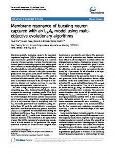
dox & Dodd, 2001) suggested that this might be due to observers’ inability to focus exclusively on reward maximization while sacrificing accuracy maximization.Because the observer must sacrifice some measure of accuracy to maximize reward when costs and benefits are manipulated, any weight placed on accuracy will lead to the use of a suboptimal decision criterion. Maddox and Bohil (1998; Maddox, 2002; Maddox & Dodd, 2001) offered a competition between reward and accuracy (COBRA) maximization hypothesis (Maddox, 2002; Maddox & Bohil, 1998; Maddox & Dodd, 2001) to (at least partially) explain this result. COBRA postulatesthat observers attempt to maximize reward (consistent with instructions and monetary compensation contingencies)but also place importance on accuracy maximization. Because the observer must sacrifice some measure of accuracy to maximize reward when payoffs are manipulated, any weight placed on accuracy will lead to the use of a suboptimal decision criterion. In a recent study, Maddox and Bohil (2001) attempted to improve decision criterion learning when costs and benefits were manipulated by reducing the weight placed on accuracy through manipulation of the trial-by-trial feedback. They speculated that observers place importance on accuracy maximization,in part, because the most common type of feedback in decision criterion learning studies emphasizes accuracy. Consider the top panel of Figure 1, which presents a hypotheticalfeedback display from a typical decision criterion learning study. Following the ob-

181

Copyright 2003 Psychonomic Society, Inc.

182

BOHIL AND MADDOX

server’s response, he or she is presented with information regarding the actual gain for that trial and the potential gain had he or she responded with the correct category label. In this example, the observer generated an incorrect B response and earned 0 points, whereas a correct A response would have earned 3 points. (In our studies, we also include information regarding cumulative performance— i.e., the total points and the potential point total.) We refer to this as objective classifier feedback, because the potential gain is always based on performance of the classifier that generates the objectively correct response on every trial and, thus, is 100% accurate. Maddox and Bohil (2001) compared decision criterion learning for objective classifier feedback with that obtained through optimal classifier feedback. The bottom panel of Figure 1 presents a hypothetical optimal classifier feedback display. Following the observer’s response, he or she is presented with information regarding the actual gain for that trial and the optimal classifier’s gain. In this example, the observer generated an incorrect B response and earned 0 points. Importantly, the optimal classifier also generated an incorrect B response and earned 0 points. Maddox and Bohil (2001) suggested that optimal classifier feedback might lead observers to sacrifice accuracy in order to maximize reward, leading to better decision criterion learning. Maddox and Bohil (2001) had each observer complete several blocks of trials in four perceptual categorization conditions that were constructed from the factorial combination of two types of feedback (optimal vs. objective classifier) with two levels of category discriminability(d ¢ = 1.0 and 2.2). All conditions used the 3:1 zero-cost payoff matrix, outlined above, and thus the optimal decision criterion was identical across all conditions. Maddox and Bohil (2001) found more nearly optimal decision criterion

learning (1) in the optimal classifier feedback condition than in the objective classifier feedback condition, with a much larger effect resulting for d ¢ = 1.0 (where the accuracy sacrifice necessary to maximize reward was large— 8%) than for d ¢ = 2.2 (where the accuracy sacrifice was small—3%), and (2) in the d ¢ = 2.2 condition than in the d ¢ = 1.0 condition. Maddox and Bohil (2001) applied a recently developed model of decision criterion learning that proposes two mechanisms that determine decision criterion placement. These will be outlined in detail below, but for now a few brief comments are in order. The first mechanism is COBRA, which postulates that observers attempt to maximize reward but also place importance on accuracy maximization. The second mechanism is based on the flatmaxima hypothesis. The flat-maxima hypothesis states that the observer’s estimate of the reward-maximizing decision criterion is determined from the objective reward function. The objective reward function plots long-run reward as a function of decision criterion placement (see Figures 3– 5). Steep objective reward functions, for which large changes in reward are associated with small changes in the decision criterion, lead to better learning of the rewardmaximizing decision criterion than do flat objective reward functions. Several factors influence the steepness of the objective reward function, including category discriminability and payoff matrix multiplication. Payoff matrix multiplication refers to one payoff matrix’s being constructed by multiplyingall entries of another payoff matrix by a constant. As we will detail later, the objective reward function is steeper for intermediate levels of d ¢, such as d ¢ = 2.2, than for small values of d ¢, such as d ¢ = 1.0 (and large d ¢ values above 3), and is steeper for large payoff matrix multiplication factors than for smaller multiplication factors.

Figure 1. Hypothetical feedback displays for the objective classifier and optimal classifier feedback conditions.

OPTIMAL VERSUS OBJECTIVE CLASSIFIER FEEDBACK Maddox and Bohil (2001) instantiated the flat-maxima and COBRA hypotheses within the framework of a hybrid model that they used to account for decision criterion placement in their task. Briefly, the model assumes that the observer’s estimate of the reward-maximizing decision criterion is determined from the steepness of the objective reward function (i.e., the flat-maxima hypothesis). The observable decision criterion is a weighted function of the estimated reward-maximizing decision criterion and the accuracy-maximizing decision criterion. The weight denotes the emphasis placed on accuracy maximization and, thus, instantiates the COBRA hypothesis. Maddox and Bohil (2001) applied the model to their data and found that the model provided a good account of the data by assuming that the weight placed on accuracy was larger for objective than for optimal classifier feedback. This article reports the results from an experiment that replicated Maddox and Bohil (2001) by examining decision criterion learning in the 3:1 zero-cost condition for the same four feedback 3 d ¢ conditions (i.e., objective classifier feedback/d ¢ = 1.0, optimal classifier feedback/d ¢ = 1.0, objective classifier feedback/d ¢ = 2.2, and optimal classifier feedback/d ¢ = 2.2), and extends Maddox and Bohil (2001) by introducing two additional manipulations, both of which affect the entries in the payoff matrix. The first manipulation is a payoff matrix subtraction manipulation. In short, we include both the 3:1 zerocost payoff matrix and a 3:1 negative-cost payoff matrix derived by subtracting 1 point from all 3:1 zero-cost payoff matrix entries. Importantly, payoff matrix subtraction does not affect the value of the optimal decision criterion, nor does it affect the steepness of the objective reward function. However, as was suggested by Maddox and Dodd (2001; see also Maddox & Bohil, 2000), decision criterion learning is more suboptimal in negative cost conditions than in zero-cost conditions, which may be due to an increased emphasis on accuracy maximization in negativecost conditions.The second manipulationis payoff matrix multiplication. In short, we include the 3:1 zero- and 3:1 negative-cost payoff matrices outlined above and two additional matrices derived by multiplying each 3:1 zerocost and each 3:1 negative-cost payoff matrix entry by a factor of 6. Like payoff matrix subtraction, payoff matrix multiplication does not affect the value of the optimal decision criterion; unlike payoff matrix subtraction, it does affect the steepness of the objective reward function. Multiplication by a factor of 6 yields a steeper objective reward function. In light of this fact, we will refer to the original payoff matrices as the 3:1 zero-cost/shallow and 3:1 negative-cost/shallow payoff matrix conditions and the two derived from payoff matrix multiplication as the 3:1 zero-cost/steep and 3:1 negative-cost/steep payoff matrix conditions. To summarize, the predictions are as follows. First, we predict better decision criterion learning with optimal classifier feedback than with objective classifier feedback, because there is a sacrifice in accuracy associated with re-

183

ward maximization in all conditions and optimal classifier feedback should lead the observer to be more willing to sacrifice accuracy in order to maximize reward. Second, we predict an interaction between the nature of the feedback and category d ¢, with a larger effect of feedback being predicted in the d ¢ = 1.0 than in the d ¢ = 2.2 conditions. This follows because the accuracy sacrifice necessary to maximize reward is larger for d ¢ = 1.0 (8%) than for d ¢ = 2.2 (3%). Third, we predict no interaction between the nature of the feedback and the payoff matrix multiplication, because payoff matrix multiplication does not affect the magnitude of the accuracy sacrifice necessary to maximize reward. Fourth, we predict better decision criterion learning for zero- than for negative-cost conditions, because observers place more weight on accuracy when losses are associated with incorrect responding. We have no a priori prediction regarding an interaction between the feedback and the payoff matrix subtraction manipulations, but it is possible that optimal classifier feedback will have an even larger effect on decision criterion learning for negative-cost conditions. Finally, we predict better decision criterion learning for the d ¢ = 2.2 than for the d ¢ = 1.0 conditions and for the steep payoff matrix multiplication conditions than for the shallow payoff matrix multiplication conditions,as would be expectedfrom the flat-maxima hypothesis. Initial tests of these predictions are provided by examining trends in performance measures, such as accuracy, points, and decision criterion estimates from signal detection theory, using analysisof variance(ANOVA). A more detailedunderstandingof the psychologicalprocesses involved in decision criterion learning under these conditions is provided by applying a series of models to the data from all conditions simultaneously, but separately by observer and block. The next (second) section will outline briefly the optimal classifier and our modeling framework. The third section will introduce Maddox and Dodd’s (2001) theory of decision criterion learning and will generate predictions from the model for the experimental factors of interest. The fourth section will be devoted to the experimental method, and the fifth section to the results and theoretical analyses. Finally, we will conclude with some general comments. THE OPTIMAL CLASSIFIER AND DECISION BOUND THEORY Optimal Classifier The optimal classifier is a hypotheticaldevice that maximizes long-run expected reward. Suppose a medical doctor must classify a patient into one of two disease categories, A or B, on the basis of medical test X, whose outcomes for Diseases A and B are normally distributed as depicted in Figure 2. Figures 2A and 2B depict hypothetical disease categories for two levels of discriminability, d ¢ = 1.0 and 2.2. The optimal classifier has perfect knowledge of the form and parameters of each category

184

BOHIL AND MADDOX

Figure 2. Hypothetical Category A and B distributions for d ¢ = 1.0 and d ¢ = 2.2. The b = 1 decision criterion, or equal-likelihood decision criterion, is optimal when category payoffs are symmetric (i.e., unbiased). The bo = 3 decision criterion is optimal when the ratio is 3:1.

distribution and records perfectly the test result, denoted x. This information is used to construct the optimal decision function, which is the likelihood ratio of the two category distributions: 1o ( x ) = f ( x B)

/ f ( x A),

(1)

where f (x | i) denotes the likelihood of test result x given disease category i. The optimal classifier has perfect knowledge of the costs and benefits in the payoff matrix. This information is used to construct the optimal decision criterion:

[

]

b o = (VaA - VbA ) / (VbB - VaB ) ,

(2)

where VaA and VbB denote the benefits associated with correct diagnoses and VbA and VaB denote the costs associated with incorrect diagnoses.2 (The category base rates affect the optimal decision criterion, but in the present study, the base rates are equal and thus drop out of the equation.) The optimal classifier (e.g., Green & Swets, 1966) uses lo(x) and bo to construct the optimal decision rule: If lo(x) . bo, then respond “B”; otherwise respond “A.” (3) Two points are in order. First, when (VaA – VbA) = (VbB – VaB), bo = 1, the optimal classifier assigns the stimulus to the category with the highest likelihood.Under these conditions, bo = 1 simultaneously maximizes reward and accuracy. Second, if the payoff for Disease A is three times the payoff for Disease B—a 3:1 payoff condition [i.e., if (VaA – VbA) = 3(VbB – VaB)]—then bo = 3.0 (see Figure 2). In this case, the optimal classifier will generate a Disease A diagnosis unless the likelihood of Disease B is at least

three times larger than the likelihood of Disease A. Importantly, although bo = 3.0 maximizes reward in this case, b = 1 maximizes accuracy. Thus, the optimal classifier must sacrifice some measure of accuracy in order to maximize reward when the payoffs are manipulated. Decision Bound Theory The optimal classifier decision rule (Equation 3) has been rejected as a model of human performance, but performance often approaches that of the optimal classifier as the observer gains experience with the task. Ashby and colleagues argued that the observer attempts to respond by using a strategy similar to that of the optimal classifier but fails because of at least two sources of suboptimality in perceptual and cognitive processing: perceptual and criterial noise (Ashby, 1992a; Ashby & Lee, 1991; Ashby & Maddox, 1993, 1994; Ashby & Townsend, 1986; Maddox & Ashby, 1993). Perceptual noise refers to trial-by-trial variability in the perceptual information associated with each stimulus. With one perceptual dimension, the observer’s percept of Stimulus i, on any trial, is given by xpi = xi + ep, where xi is the observer’s mean percept and ep is a random variable denoting perceptual noise (we assume that spi = sp). Criterial noise refers to trial-by-trial variability in the placement of the decision criterion. With criterial noise, the decision criterion used on any trial is given by bc = b + ec, where b is the observer’s average decision criterion and ec is a random variable denoting criterial noise (assumed to be univariate normally distributed). Decision bound theory assumes that the observer attempts to use the same strategy as the optimal classifier, but with less success, owing to the effects of perceptual and criterial noise. Hence, the simplest decision bound model is the

OPTIMAL VERSUS OBJECTIVE CLASSIFIER FEEDBACK

185

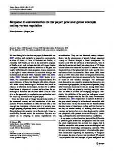
optimal decision bound model. The optimal decision bound model is identical to the optimal classifier (Equation 3), except that perceptual and criterial noise are incorporated into the decision rule. Specifically, If lo(xpi) . bo + ec, then respond “B”; otherwise respond “A.” (4) A THEORY OF DECISION CRITERION LEARNING AND A HYBRID MODEL FRAMEWORK Maddox and Dodd (2001; Maddox, 2002) offered a theory of decision criterion learning and a model-based instantiationcalled the hybrid model. The theory proposestwo mechanisms that determine decision criterion placement. Flat-Maxima Hypothesis The first mechanism is based on the flat-maxima hypothesis (Busemeyer & Myung, 1992; vonWinterfeldt & Edwards, 1982).As has been suggestedby many researchers, suppose that the observer adjusts the decision criterion (at least in part) on the basis of the change in the rate of reward, with larger changes in rate being associated with faster, more nearly optimal decision criterion learning (e.g., Busemeyer & Myung, 1992; Dusoir, 1980; Kubovy & Healy, 1977; Thomas, 1975; Thomas & Legge, 1970). To formalize this hypothesis, one can construct the objective reward function. The objective reward function plots objective expected reward on the y-axis and the decision criterion value on the x-axis (e.g., Busemeyer & Myung, 1992; Stevenson, Busemeyer, & Naylor, 1991; vonWinterfeldt & Edwards, 1982). To generate an objective reward function, one chooses a value for the decision criterion and computes the long-run expected reward for that criterion value. This process is repeated over a range of criterion values. The expected reward is then plotted as a function of decision criterion value. Figure 3A plots expected reward as a function of the deviation between a hypothetical observer’s decision criterion ln(b) and the optimal decision criterion ln(bo) standardized by category d ¢. This is referred to as k 2 ko = ln(b)/d ¢ 2 ln(bo)/d ¢. Note that for large deviations from the optimal decision criterion, the expected reward is small and that, as the deviation from the optimal decision criterion decreases, the expected reward increases. Note also that when the deviation from optimal is zero (i.e., when the decision criterion is the optimal decision criterion), expected reward is maximized. The derivative of the objective reward function at a specific k 2 ko value determines the change in the rate of expected reward for that k – ko value; the larger the change in the rate, the “steeper” the objective reward function at that point. Derivatives for three k 2 ko values are denoted by Tangent Lines 1, 2, and 3 in Figure 3A. Note that the slope of each tangent line, which corresponds to the derivative of the objective reward function at that point, decreases as the deviation from the optimal decision criterion decreases (i.e., as we go from Point 1 to 2 to 3). In other words, the change in the rate of reward or steepness

Figure 3. (A) Expected reward as a function of the decision criterion (relative to the optimal decision criterion; i.e., k 2 k o ), called the objective reward function. The three lines are the tangent lines at points 1, 2, and 3 on the objective reward function that denote the derivative or steepness of the objective reward function at each point. (B) Steepness of the objective reward function from panel A, along with the three points highlighted in panel A.

declines as the decision criterion approaches the optimal decision criterion. Figure 3B plots the relationship between the steepness of the objective reward function (i.e., the derivative at several k – ko values) and k – ko. The three derivatives denoted in Figure 3A are highlighted in Figure 3B. If the observer adjusts the decision criterion on the basis of the change in the rate of reward (or steepness), steeper objective reward functions should be associated with more nearly optimal decision criterion values, be-

186

BOHIL AND MADDOX each objective reward function (i.e., the derivatives of each objective reward function) and k 2 ko. The tangent lines (labeled “1”) in Figure 4A correspond to the k 2 ko values associated with the same fixed steepness value for d ¢ = 1.0 and 2.2, respectively. The horizontal line (labeled “1”) in Figure 4B denotes the same fixed nonzero steepness value, and the vertical lines denote the associated k 2 ko values for each condition. Two comments are in order. First, note that the four objective reward functions in Figure 4A collapse onto two steepness functions in Figure 4B because the steepness of the objective reward function is

Figure 4. (A) Objective reward functions for 3:1 zero-cost and 3:1 negative-cost payoff matrices for d ¢ = 1.0 and d ¢ = 2.2. The tangent lines (labeled “1”) correspond to the same steepness value on each function. (B) Steepness of the objective reward functions for each d ¢ value in panel A (see text for explanation), along with the points highlighted in panel A.

cause only a small range of decision criterion values around the optimal value have near-zero derivatives (or small steepness values). Flat objective reward functions, on the other hand, will lead to less optimal decision criterion placement, because a larger range of decision criterion values around the optimal value have derivatives near zero. Category discriminability, payoff matrix subtraction, payoff matrix multiplication, and the flatmaxima hypothesis. Figure 4A displays the objective reward functions for category d ¢ = 1.0 and 2.2 with both the 3:1 zero-cost and the 3:1 negative-cost payoff matrices. Figure 4B plots the relationship between the steepness for

Figure 5. (A) Objective reward functions for payoff matrix muliplication (PMM) factors 1 and 6 for d ¢ = 1.0 and d ¢ = 2.2. The tangent lines (labeled “1”) correspond to the same steepness value on each function. (B) Steepness of the objective reward functions from panel A, along with the points highlighted in panel A.

OPTIMAL VERSUS OBJECTIVE CLASSIFIER FEEDBACK unaffected by payoff matrix subtraction. Second, note that the deviation between the decision criterion and the optimal value, k 2 ko, differs systematically across category d ¢ conditions in such a way that the decision criterion, k, is closer to the optimal value, ko, for category d ¢ = 2.2 than for d ¢ = 1.0. Thus, the flat-maxima hypothesis predicts that performance should be closer to optimal for d ¢ = 2.2 than for d ¢ = 1.0. Figure 5A displays the objective reward functions for the steep and shallow 3:1 zero-cost payoff matrices for category d ¢ = 1.0 and 2.2. The objective reward functions associated with the 3:1 negative-cost payoff matrices are omitted, since they share equivalentsteepness values with their 3:1 zero-cost matrix counterparts. Figure 5B plots the relationship between the steepness for each objective reward function (i.e., the derivatives of each objective reward function) and k 2 ko. The tangent lines in Figure 5A (labeled “1”) denote the k 2 ko values associated with the same fixed steepness value on all four objective reward functions. The horizontal line (labeled “1”) in Figure 5B denotes the same fixed nonzero steepness value, and the vertical lines denote the associated k 2 ko values for each condition. Note that k 2 ko is smaller for conditions in which the payoff matrix multiplication factor is 6 and, as in Figure 4B, for d ¢ = 2.2 than for d ¢ = 1.0. Because the flat-maxima hypothesis is based on the objective reward function, it applies only to learning of the reward-maximizing decision criterion. The observed decision criterion is assumed to be a weighted average of the reward- and accuracy-maximizing decision criteria. The COBRA hypothesis instantiates the weighting process. COBRA Hypothesis The second mechanism assumed to influence decision criterion placement is based on Maddox and Bohil’s (1998) COBRA maximization hypothesis. COBRA postulates that observers attempt to maximize expected reward (consistent with instructions and monetary compensation contingencies) but that they also place importance on accuracy maximization. Consider the univariate categorization problem depicted in Figure 6 with a 3:1 payoff ratio.

187

Note that the reward-maximizing decision criterion, kro = ln(b ro)/d ¢ = ln(3)/d ¢ is different from the accuracymaximizing decision criterion, kao = ln(bro)/d ¢ = ln(1)/d, and, thus, the observer cannot simultaneously maximize accuracy and reward. If an observer places importance or weight on reward and accuracy, the resulting decision criterion will be intermediate between the reward- and the accuracy-maximizing criteria. We instantiate this process with a simple weighting function, k = wka + (1 2 w)kr, where w (0 # w # 1) denotes the weight placed on accuracy. This weighting function results in a single decision criterion that is intermediate between that for accuracy maximization and that for reward maximization.3 For example, in Figure 6, k1 denotes a case in which w , .5, whereas k2 denotes a case in which w . .5. An accuracy weight of w , .5 might correspond to a situation in which feedback is based on the optimal classifier, and an accuracy weight of w . .5 might correspond to a situation in which feedback is based on the objective classifier. Framework for a Hybrid Model Maddox and Dodd (2001) developed a hybrid model of decision criterion learning that incorporated both the flatmaxima and the COBRA hypotheses. To facilitate development of the model, consider the following equation that determines the decision criterion used by the observer on condition i trials (ki): k i - wk a + (1 - w ) k r .

(5)

The model assumes that the decision criterion used by the observer to maximize expected reward (kr) is determined by the steepness of the objective reward function (see Figures 3–5). A single steepness parameter is estimated from the data that determines a distinct decision criterion in every condition for which the steepness of the objective reward function differs. The accuracy-maximizing decision criterion, ka, is associated with the equal likelihood criterion. Before each experimental condition, the observer is pretrained on the category structures in a baseline condition with equal payoffs (described in the Method section), which pretrains the accuracy-maximizing decision crite-

Figure 6. Schematic illustration of the competition between reward and accuracy (COBRA) hypothesis. The reward-maximizing criterion is denoted by k ro. The accuracymaximizing criterion is denoted by kao . Criterion k 1 represents a criterion that results if the subject places more weight on reward than on accuracy (i.e., w < .5), whereas criterion k2 represents the case in which accuracy is more heavily weighted than reward (i.e., w > .5).

188

BOHIL AND MADDOX

rion. This criterion is then entered into the weighting function, along with the observer’s estimate of the rewardmaximizing decision criterion, to determine the criterion used on each trial. The COBRA hypothesis is instantiated in the hybrid model by estimating the accuracy weight, w, from the data. It is important to make a clear distinction between predictions that can be derived mathematically from the theory and those that are not based on a mathematical derivation but, instead, are based on a body of empirical evidence or on a sensible assumption. All predictions associated with the flat-maxima hypothesis are mathematically derived. For example, as is suggested by Figures 3–5, k 2 ko is smaller for d ¢ = 2.2 than for d ¢ = 1.0 and is smaller for steep than for shallow payoff matrices. The COBRA prediction that the observed decision criterion must fall somewhere between the accuracy-maximizing, b 5 1 criterion and the reward-maximizing decision criterion derived from the flat-maxima hypothesis is also mathematically derived (Equation 5). On the other hand, it is reasonable to assume (and test) the hypothesis that decision criterion learning is worse when negative costs are present or for objective classifier feedback, but these predictions are not derivable mathematically. All of the models developed in this article are based on the decision bound model in Equation 4. Each model includes two noise parameters (one for d ¢ = 1.0 and one for d ¢ = 2.2) that represent the sum of perceptual and criterial noise (Ashby, 1992a; Maddox & Ashby, 1993). Each

model assumes that the observer has accurate knowledge of the category structures [i.e., lo(xpi )]. To ensure that this was a reasonable assumption, each observer completed a number of baseline trials and was required to meet a stringent performance criterion (see the Method section). Finally, each model allows for suboptimal decision criterion placement where the decision criterion is determined from the flat-maxima hypothesis, the COBRA hypothesis, or both following Equation 5. To determine whether the flatmaxima and the COBRA hypotheses are important in accounting for each observer’s data, we developed four models. Each model makes different assumptions about the kr and w values. The nested structure of the models is presented in Figure 7, with each arrow pointing to a more general model and models at the same level having the same number of free parameters. The number of free parameters (in addition to the noise parameter described above) is presented in parentheses. (The details of the model-fitting procedure are outlined in the Results section.) The optimal model instantiates neither the flat-maxima nor the COBRA hypothesis. It assumes that the decision criterion used by the observer to maximize expected reward is the optimal decision criterion (i.e., kr = ko) and that there is no competition between reward and accuracy maximization (i.e., w = 0). The flat-maxima model instantiates the flat-maxima hypothesis, but not the COBRA hypothesis, by assuming that the decision criterion used by the observer to maximize expected reward (kr) is determined by the steepness of the objective reward func-

Figure 7. Nested relationship among the decision bound models applied simultaneously to the data from all experimental conditions. Each arrow points to a more general model. Note: All models assume two free noise parameters (one per d ¢ ).

OPTIMAL VERSUS OBJECTIVE CLASSIFIER FEEDBACK tion, as in Figures 3–5, and that there is no competitionbetween reward and accuracy maximization (i.e., w = 0). A single steepness parameter is estimated from the data. The flat-maxima model contains the optimal model as a special case. The COBRA model instantiates the COBRA hypothesis, but not the flat-maxima hypothesis by assuming that kr = ko, while allowing for a competition between reward and accuracy maximization by estimating the Equation 5 w parameter from the data. This model contains the optimal model as a special case. The hybrid(w) model instantiates both the flat-maxima and the COBRA hypotheses by assuming that kr is determined by the steepness of the objective reward function and that there is a competition between accuracy and reward maximization. This model contains the previous three models as special cases. Three more general versions of the hybrid model were applied to the data to test specific predictions. The hybrid (wObjective ; wOptimal ) model estimated two accuracy weights: One was applied to all objective classifier feedback conditions, and the other to all optimal classifier feedback conditions.This model was developed to test the main prediction that optimal classifier feedback leads to better decision criterion learning by reducing the weight placed on accuracy maximization. The hybrid (w Objective/d ¢=1.0; wOptimal/d ¢=1.0; w Objective/d ¢=2.2; wOptimal/d ¢=2.2) model estimated four accuracy weights: one for the objective classifier feedback/d ¢ = 1.0 conditions,a second for the optimal classifier feedback/d ¢ = 1.0 conditions, a third for the objective classifier feedback/d ¢ = 2.2 conditions,and a fourth for the optimal classifier feedback/d ¢ = 2.2 conditions. This model was developed to test the prediction that the effect of optimal classifier feedback, relative to objectiveclassifier feedback, would be larger for d ¢ = 1.0 than for d ¢ = 2.2. Finally, the hybrid(8w) model estimated the same four accuracy weightsas those outlinedin the hybrid(wObjective/d ¢=1.0; wOptimal/d ¢=1.0; wObjective/d ¢=2.2; wOptimal/d ¢=2.2) model but estimated one set of four accuracy weights for the steep payoff matrix multiplication conditions and a separate set of four weights for the shallow payoff matrix multiplication conditions,yielding a total of eight accuracy weights. Since we did not predict an interaction between payoff matrix multiplication and feedback condition, we did not expect

this model to provide a statistically significant improvement in fit over the more restricted hybrid(wObjective/d ¢=1.0; wOptimal/d ¢=1.0; wObjective/d ¢=2.2; wOptimal/d ¢=2.2) model. EXPERIMENT The overriding goal of this experiment was to examine the differential effects of objective-versus optimal-classifier feedback on decision criterion learning in 3:1 zero-cost and 3:1 negative-cost conditions at two levels of category discriminability for two payoff matrix multiplication factors. Each observer completed 16 perceptual categorization tasks constructed from the factorial combination of 2 types of feedback (optimal classifier and objective classifier) with 2 payoff matrix subtraction conditions(3:1 zero cost and 3:1 negative cost), 2 levels of d ¢ (1.0 and 2.2), and two payoff matrix multiplication conditions (multiplication by a factor of 1 or 6). Each task consisted of three 120-trial blocks of training in which trial-by-trial feedback was based on the optimal classifier or the objective classifier, followed by a 120-trial test block, during which feedback was omitted. Table 1 displays the payoff matrix values, optimal points, optimal accuracy, and optimal decision criterion value for each experimental condition for a single block of trials. Method Observers Eight observers were recruited from the University of Texas community. All observers claimed to have 20/20 vision or vision corrected to 20/20. Each observer completed 16 sessions, each of which lasted approximately 60 min. Monetary compensation was based on the number of points accrued across the whole experiment. Stimuli and Stimulus Generation The stimulus was a filled white rectangular bar (40 pixels wide) presented on the black background of a computer monitor. The bar rested upon a stationary base (60 pixels wide) that was centered on the screen, and bar height varied from trial to trial. There were two categories, A and B, whose members were sampled from separate univariate normal distributions. The sampled values determined the height of each presented bar stimulus. Category mean separation was 21 and 46 pixels for d ¢ = 1.0 and d ¢ = 2.2 conditions, respectively. The standard deviation was 21 pixels for each category. Sev-

Table 1 Category Payoff Matrix Entries, Points, Accuracy, and Optimal Decision Criterion Value (Based on 120-Trial Blocks) for Each Experimental Condition Payoff Matrix Entries Condition

VaA

VbB

189

VbA

VaB

Points

Accuracy

bo

0 21 0 26

186 66 1116 396

60.99 60.99 60.99 60.99

3 3 3 3

0 21 0 26

212 92 1272 552

82.94 82.94 82.94 82.94

3 3 3 3

3:1 zero-cost/shallow 3:1 negative-cost/shallow 3:1 zero-cost/steep 3:1 negative-cost/steep

3 2 18 12

1 0 6 0

d ¢ = 1.0 0 21 0 26

3:1 zero-cost/shallow 3:1 negative-cost/shallow 3:1 zero-cost/steep 3:1 negative-cost/steep

3 2 18 12

1 0 6 0

d ¢ = 2.2 0 21 0 26

190

BOHIL AND MADDOX

eral random samples of a size of 60 were taken from each distribution, and the samples that best reflected the population means, standard deviations, and objective reward function were selected to yield a set of 120 unique stimuli for each level of d ¢. Procedure Prior to the first experimental session, the observers were informed that they would be participating in a series of simulated medical diagnosis tasks and that, on each trial of the experiment, they would see a bar graph presented on the computer screen. They were told that the bar represented the result of a hypothetical medical test that was predictive of two possible diseases and that their job was to try to diagnose the patient on the basis of this test result (i.e., the height of the bar). The observers were told that each trial represented the test result for a new patient and that they would earn a certain number of points for each trial, depending on how they responded. They were instructed to try to maximize their point total over the course of the experiment, since this would determine their monetary compensation. The order of presentation for the 16 experimental conditions was determined by Latin square, and the observers completed one experimental condition during each daily session. To teach the observers the category distributions prior to any payoff manipulation, as well as to minimize carryover effects, each experimental condition was preceded by the completion of a minimum of 60 baseline trials, in which category costs and benefits were unbiased (i.e., VaA = 2, VbB = 2, VbA = 0, and VaB = 0) and the feedback and category discriminability matched that of the ensuing experimental condition. After completing 60 baseline trials, performance was examined. If the observer reached an accuracy-based performance criterion (response accuracy not more than 2% below optimal), those 60 trials were fit by two decision bound models (see Maddox & Bohil, 1998, for details). The optimal decision criterion model assumed that the observer used the optimal decision criterion (i.e., bo = 1) in the presence of perceptual and criterial noise (explained in the Results and Theoretical Analyses section below), whereas the free decision criterion model estimated the observer’s decision criterion, along with perceptual and criterial noise, from the data. Because the optimal decision criterion model is a special case of the free decision criterion model, likelihood ratio tests were used to determine whether the extra flexibility of the free decision criterion model provided a significant improvement in fit. If the free decision criterion model did not provide a significant improvement in fit over the optimal decision criterion model, the observer was allowed to begin the experimental condition. If the free decision criterion model did provide a significant improvement in fit, the observer completed 10 additional trials, and the same accuracy-based and model-based criteria were applied to the most recent 60 trials (i.e., Trials 11–70). This procedure continued until the observer reached the appropriate criterion. Including these baseline trials and these fairly conservative accuracybased and model-based performance criteria ensured that each observer had accurate knowledge of the category structures before exposure to the payoff manipulation and minimized the possibility of within-observers carryover effects from one experimental condition to the next. In addition, a different set of disease (i.e., category) labels was used in each experimental condition. A typical trial proceeded as follows. The stimulus was presented on the screen and remained until a response was made. The observers were instructed to categorize each stimulus by pressing the appropriate button on the keyboard. Five lines of feedback, which stayed on the screen until the observer pressed a key to move on to the next patient, followed each response. Figure 1 presents hypothetical feedback displays for optimal classifier and objective classifier feedback conditions. The top line of feedback indicated the disease possessed by the hypothetical patient (instead of the categorization response, which was depicted in Figure 1 for illustrative purposes). Fictitious disease names were used (e.g., “valinemia” or “brucellosis”), and a different pair of disease labels accompanied each ex-

perimental condition. The second line indicated the number of points gained or lost for the given response. In objective feedback conditions, the third line displayed the potential gain for a (objectively) correct response on the trial. In other words, if the observer’s response was correct on the basis of a priori category membership, lines two and three of the feedback presented the same number of points. If the observer’s response was incorrect, the third line showed what could have been earned had a correct response been given. In optimal classifier feedback conditions, however, the third line of feedback presented the number of points that the optimal classifier earned. In this case, if the observer made an (objectively) incorrect response on the basis of a priori category membership of the stimulus but gave the correct response in relation to the optimal criterion, both the observer and the optimal classifier would be incorrect for that trial, and lines two and three would present the same number of points gained or lost (see Figure 1). The fourth line showed the number of points that the observer had accumulated to that point in the experimental condition, and the fifth line showed the number of points accrued by the objective or the optimal classifier, depending on feedback condition. There was a 125-msec intertrial interval, during which the screen was blank, between removal of the feedback and presentation of the next stimulus. The observers were given a break every 60 trials, during which the monitor displayed their accumulated point total for the condition and the optimal point total (i.e., the point total that the optimal classifier would earn in the experimental condition).

Results and Theoretical Analysis Before we turn to the model-based analyses, a few words are in order regarding some basic trends in the signal detection theory decision criterion estimates (Green & Swets, 1966), point totals, and accuracy rates. Performance Trends Because decision criterion estimates, points, and accuracy are each measured on a different scale, we transformed each of these measures onto a common scale that allowed us to compare the observer’s performance with that of the optimal classifier. Specifically, we computed the following three measures: deviation from optimal decision criterion = k – ko = ln(b)/d ¢ 2 ln(bo)/d ¢,

(6)

deviation from optimal points =

(observed points - optimal points) , (optimal points - points for 0%)

(7)

and deviation from optimal accuracy (observed accuracy - optimal accuracy) . (8) (optimal - accuracy) The k – ko values (averaged across blocks) are displayed separately for each of the 16 experimental conditions and observers in Table 2. A 2 feedback (objective classifier vs. optimal classifier) 3 2 category discrminability (d ¢ = 1.0 vs. 2.2) 3 2 payoff matrix subtraction (zero-cost vs. negative cost) 3 2 payoff matrix multiplication (multiplication by a factor of 1 vs. 6) 3 4 block ANOVA was conducted separately on the decision criterion, point, and =

OPTIMAL VERSUS OBJECTIVE CLASSIFIER FEEDBACK

191

Table 2 Deviation From Optimal Decision Criterion (k – ko) for Each of the 16 Experimental Conditions and 8 Observers (Averaged Across Blocks) Observer d¢

Decision Criterion

Condition

1

2

3

4

5

6

7

8

objective

3:1 zero-cost/shallow 3:1 negative-cost /shallow 3:1 zero-cost/steep 3:1 negative-cost /steep 3:1 zero-cost/shallow 3:1 negative-cost /shallow 3:1 zero-cost/steep 3:1 negative-cost/steep

21.00 20.95 21.03 21.02 20.90 20.97 20.73 20.91

20.99 21.05 20.65 20.69 20.71 20.71 20.80 20.88

20.99 21.06 21.01 20.77 20.30 20.46 20.27 21.08

21.08 21.14 20.93 20.88 20.28 20.36 20.49 20.54

21.09 21.13 20.85 21.00 21.07 20.37 20.38 20.99

20.51 20.65 20.38 20.45 20.39 20.43 20.54 20.40

20.87 21.11 21.01 21.03 20.71 20.53 20.85 20.73

21.41 21.32 21.17 21.15 0.20 20.58 20.13 20.32

3:1 zero-cost/shallow 3:1 negative-cost/shallow 3:1 zero-cost/steep 3:1 negative-cost /steep 3:1 zero-cost/shallow 3:1 negative-cost /shallow 3:1 zero-cost/steep 3:1 negative-cost /steep

20.21 20.20 20.19 20.29 20.35 20.34 20.33 20.39

20.33 20.45 20.13 20.09 20.43 20.46 20.26 20.12

20.40 20.59 20.32 20.32 20.10 20.42 20.17 20.33

20.14 20.50 20.20 20.36 20.48 20.32 20.21 20.43

20.32 20.34 20.41 20.33 20.36 20.17 20.33 20.15

0.04 0.08 20.20 0.08 20.13 20.08 20.12 20.01

20.45 20.57 20.27 20.10 20.45 20.22 20.32 20.13

20.25 0.04 20.20 20.29 20.10 20.33 20.10 0.02

1.0

optimal

2.2 objective

optimal

accuracy deviation scores. We predicted a main effect of feedback type and a feedback type 3 category d ¢ interaction in which the magnitude of the feedback effect was predicted to be larger for d ¢ = 1.0 than for d ¢ = 2.2. The main effect of feedback type was significant for the decision criterion measure [F(1,7) = 7.29, MSe = 3.63, p , .05], was significant at the p = .08 level for the point measure [F(1,7) = 4.09, MSe = 0.01, p = .08], but was nonsignificant for the accuracy measure. The feedback type 3 category d ¢ interaction was significant for both the decision criterion and the point measures [decision criterion, F(1,7) = 10.13, MSe = 0.36, p , .05; point, F(1,7) = 10.56, MSe = 0.01, p , .05] and revealed a larger feedback effect for d ¢ = 1.0 than for d ¢ = 2.2. This effect can be seen graphically in Figure 8, which depicts the decision criterion, point, and accuracy measures for objective and optimal classifier feedback separately for the two levels of category d ¢ and payoff matrix subtraction. We predicted a main effect for payoff matrix subtraction, with better performance being predicted in the zero-cost conditions.This effect was significant only for the point measure [F(1,7) = 7.83, MSe = 0.002, p , .05] but was qualified by a significant payoff matrix subtraction 3 category d ¢ interaction for the decision criterion measures [decision criterion, F(1,7) = 6.51, MSe = 0.03, p , .05] and a significant interaction at the p = .09 level for the point measure [F(1,7) = 3.75, MSe = 0.002, p = .09]. Similar to the feedback type 3 category d ¢ interaction,the payoff matrix subtraction3 category d ¢ interaction revealed a larger effect of payoff matrix subtraction for d ¢ = 1.0 than for d ¢ = 2.2, with worse performance resulting for the negative-cost conditions. This result is depicted in Figure 8. We also predicted a main effect of category d ¢ in which performance was predicted to be closer to optimal for d ¢ = 2.2 than for d ¢ = 1.0. This effect was significant for all three performance measures and is depictedin Figure 8 [decision criterion, F(1,7) =

186.86, MSe = 0.16, p , .001; point, F(1,7) = 45.83, MSe = 0.01, p , .001; accuracy, F(1,7) = 37.49, MSe = 0.02, p , .001]. Finally, we predicted a main effect of payoff matrix multiplication,which was observed for the decision criterion and point measures [decision criterion, F(1,7) = 13.76, MSe = 0.05, p , .01; point: F(1,7) = 6.34, MSe = 0.003, p , .05]. As was predicted, performance was closer to optimal when the payoff matrix multiplication factor was 6 (deviation from optimal decision criterion = 2.51; deviation from optimal points = 2.057) than when the payoff matrix multiplication factor was 1 (deviation from optimal decision criterion = 2.58; deviation from optimal points = 2.069). A main effect of block was also observed for the decision criterion and point measures [decision criterion, F(3, 21) = 4.68, MSe = 0.09, p , .05; point, F(3, 21) = 3.49, MSe = 0.003, p , .05]. Performance gradually improved across the three training blocks, then showed a small decrement in performance in the final test block. We speculated that an interaction might emerge between feedback type and payoff matrix subtraction, but an interaction was not found for any of the three performance measures. Other interaction effects were observed, but these rarely held for more than one performance measure and were not of theoretical interest. These ANOVA results provide good initial support for the many predictions outlined in the introduction and provide a foundation for the stronger model-based analyses that we turn to next. Model-Based Analyses Each of the models shown in Figure 7 was applied simultaneously to the data from all 16 experimental conditions separately for each block and observer. Each block consisted of 120 experimental trials, and the observer was required to respond “A” or “B” for each stimulus. Thus, each model was fit to a total of 1,920 response probabili-

192

BOHIL AND MADDOX

Figure 8. Deviation from optimal decision criterion (top panel), points (middle panel), and accuracy (bottom panel) for the objective and optimal classifier feedback conditions by zero versus negative cost and category d ¢ condition averaged across payoff matrix multiplication, block, and observer. Standard error bars are included.

ties from each block (120 trials 3 16 conditions). Maximum likelihood procedures (Ashby, 1992b; Wickens, 1982) were used to estimate the model parameters, and likelihood ratio (G2) tests were used to determine whether a more general model provided a significant improvement in fit (with a = .05) over a more restricted, nested model.4 Because the models were applied separately to each block of trials, we could identify the model with the fewest free parameters that could not be improved upon (statistically) by a more general model, referred to as the most parsimonious model, for each observer in each block. However, our interest was in identifying the most parsimonious model overall for each observer. Since decision criterion shifts across trials are likely large early in learning but are

much smaller later in learning and during the test block, we decided to determine the most parsimonious model from the final training block and the test block. Thus, the G2 tests were based on the fit of each model summed over the last two blocks. (Using the cumulative fit across all four blocks did not change the overall pattern of results.) Even so, we do examine the parameter values separately for each block in order to better characterize decision criterion changes with experience. On the basis of likelihood ratio (G 2) tests of the maximum likelihood f it values, the hybrid(w Objective/d ¢=1.0; wOptimal/d ¢=1.0; wObjective/d ¢=2.2; wOptimal/d ¢=2.2) model that predicted an interaction between the type of feedback and category d ¢ in the weight placed on accuracy maximiza-

OPTIMAL VERSUS OBJECTIVE CLASSIFIER FEEDBACK tion provided the most parsimonious account of the data from 4 of the 8 observers. The hybrid(w) model that assumed a fixed accuracy weight in all conditions was most parsimonious for 2 of the 8 observers, and the hybrid(8w) model that assumed a three way interaction between the type of feedback, category d ¢, and payoff matrix multiplication was most parsimonious for the remaining 2 observers. The fact that the hybrid models were superior for all 8 observers suggests that both hypotheses—the flatmaxima and the COBRA hypotheses—are necessary to provide an adequate account of human decision criterion learning. The relatively poor showing of the most general hybrid(8w) model supports the prediction that payoff matrix multiplication does not interact with the effects of feedback type and category d ¢. It also suggests that the models are capturing meaningful trends in the data and are not just over-fitting the data, as one might expect when the most general model provides a consistently superior account of the data. The strong showing for the hybrid (wObjective/d ¢=1.0; wOptimal/d ¢=1.0; wObjective/d ¢=2.2; wOptimal/d ¢=2.2) model suggests that an interaction did emerge between the type of feedback and category d ¢. To determine how the observer’s estimate of the rewardmaximizing decision criterion changed across blocks, we examined the steepness parameters from the hybrid (wObjective/d ¢=1.0; wOptimal/d ¢=1.0; wObjective/d ¢=2.2; wOptimal/d ¢=2.2) model. These values are displayed in the top panel of Figure 9. To determine the magnitude of the weight placed on accuracy, how it was affected by the nature of the feedback and category d ¢, and how it changed across blocks, we examined the accuracy weight, w, parameters from the hybrid(w Objective/d ¢=1.0; w Optimal/d ¢=1.0; w Objective/d ¢=2.2; wOptimal/d ¢=2.2) model. These values are displayed in the bottom panel of Figure 9. A one-way ANOVA on the steepness values suggested no effect of block. A 2 feedback type (objective classifier vs. optimal classifier) 3 2 category discriminability (d ¢ = 1.0 vs. d ¢ = 2.2) 3 4 block ANOVA was conducted on the accuracy weight values. Several results stand out. First, there was a main effect of feedback type [F(1,7) = 5.50, MSe = 0.13, p = .05], revealing a smaller accuracy weight for optimal classifier feedback (w = .46) than for objective classifier feedback (w = .60). Second, there was a main effect of category d ¢ [F(1,7) = 15.62, MSe = 0.07, p , .01], revealing a smaller accuracy weight for d ¢ = 2.2 (w = .44) than for d ¢ = 1.0 (w = .62). Third, there was a feedback type 3 block interaction [F(3,21) = 3.80, MSe = 0.02, p , .05] that suggested a gradual decline in the accuracy weight across training blocks (which did not hold into the test block) for optimal classifier feedback, but not for objective classifier feedback. This is an important finding because it suggests that observers became more willing to sacrifice accuracy as they gained experience with the task when feedback was based on the optimal classifier. Perhaps, given enough exposure to optimal classifier feedback, observers could eventually learn to completely sacrifice accuracy maximization, like the optimal classifier. Fourth, the most striking finding from an examination of Fig-

193

ure 9B was that the weight placed on accuracy was (statistically) equivalent in the d ¢ = 1.0 and d ¢ = 2.2 optimal classifier feedback conditions and the d ¢ = 2.2 objective classifier condition but was significantly larger in the d ¢ = 1.0 objective classifier condition. This finding supports the prediction that the effect of optimal classifier versus objective classifier feedback should be greatest when the accuracy sacrifice necessary to maximize reward was large. Finally, it is important to note that the fit of the model was quite good with the hybrid(w Objective/d ¢=1.0; w Optimal/d ¢=1.0; wObjective/d ¢=2.2; wOptimal/d ¢ =2.2) model, accounting for 85.7%– 93.0% of the responses in the data from the 8 observers. Two Alternative Explanations The good fit of the hybrid(wObjective/d ¢=1.0; wOptimal/d ¢=1.0; wObjective/d ¢=2.2; wOptimal/d ¢=2.2) model to each observer’s data supports the claim that optimal classifier feedback leads observers to sacrifice accuracy in the interest of reward maximization. Even so, at least three alternative explanations are available (we are indebted to Ido Erev [August, 2002, personal communication] for suggesting these alternatives). We outline and address each in turn. Release from equal category response frequency hypothesis. As was outlined earlier, conservative cutoff placement is commonly observed when either base rates or costs–benefits are manipulated. One possibility is that observers have a tendency to be fair and unbiased in their responding. Specifically, observers have a bias to give each categorization response with equal frequency and, thus, are biased toward b = 1. Optimal classifier feedback might “release” observers from this bias, allowing them to generate one response more than the other and leading to more nearly optimal decision criterion learning. When costs and benefits are manipulated, as in the present experiment, the equal response frequency decision criterion and the accuracy-maximizing decision criterion are identical and are set at b 5 1. Since the release from equal category response frequency hypothesis assumes that optimal classifier feedback allows the observer to shift away from b 5 1 and since COBRA assumes that optimal classifier feedback leads the observer to place less weight on accuracy maximization, both hypotheses make identical predictions. However, when category base rates are unequal, the two hypotheses make different predictions. When base rates are manipulated, the equal response frequency decision criterion is set at b 5 1, but the accuracyand reward-maximizing decision criteria are identical and are set at b 5 3. Thus, the release from equal category response frequency hypothesis continues to predict better decision criterion learning for optimal classifier feedback, whereas the COBRA hypothesis predicts no effect of optimal versus objective classifier feedback on decision criterion learning, because the accuracy- and reward-maximizing decision criteria are identical, effectively eliminating competition (see Maddox & Bohil, 1998, for a detailed discussion). To summarize, the release from equal category response frequency hypothesis predicts better decision

194

BOHIL AND MADDOX

Figure 9. (A) Steepness values and (B) accuracy weight, w, values from the hybrid(wObjective/d ¢=1.0 ; wOptimal/d ¢=1.0 ; wObjective/d ¢=2.2 ; w Optimal/d ¢=2.2 ) model for the three training blocks and the test block, averaged across observers. Standard error bars are included.

criterion learning with optimal classifier feedback relative to objective classifier feedback for 3:1 cost–benefit conditions and 3:1 base rate conditions.COBRA, on the other hand, predicts better decision criterion learning with optimal classifier feedback relative to objective classifier feedback for 3:1 cost–benefit conditions, but no performance difference across optimal and objective feedback types for 3:1 base rate conditions. As a test of these hypotheses, we collected data from 40 observers who each completed one session (i.e., a minimum of 60 baseline trials, followed by three 120-trial blocks of training, and one 120-trial test block) in a 3:1 base rate condition. Ten observers participated in each of four conditions constructed from the factorial combination of optimal versus objective classifier feedback with d ¢ = 1.0 versus d ¢ = 2.2. Because we used a betweenobservers design, the models shown in Figure 7 could not be applied to the data. Even so, we examined the deviation from optimal decision criterion (k 2 ko) values from the

3:1 base rate study and compared these values with those observed in the 3:1 zero-cost/shallow payoff matrix from the experiment outlined above (within-observers design) and with those observed in Maddox and Bohil’s (2001) Experiment 1 (between-observers design). These values are displayed graphically in Figure 10, averaged across the final two blocks (i.e., the final training block and the test block) and d ¢ levels. The most important finding was the performance advantage for optimal classifier feedback, relative to objective classifier feedback, in the two 3:1 payoff experiments that was not observed in the 3:1 base rate condition.This pattern of results supports the COBRA hypothesis over the release from equal category response frequency hypothesis. A related hypothesis can be developed that assumes a competition between reward maximization and probability matching instead of a competition between reward and accuracy maximization (COBRA). Equation 5 instantiates the hypothesis that there is a competition between reward

OPTIMAL VERSUS OBJECTIVE CLASSIFIER FEEDBACK

195

Figure 10. Deviation from optimal decision criterion (k 2 ko) from the 3:1 base rate, between-observers design, 3:1 zero-cost/shallow payoff matrix, between-observers design (Maddox & Bohil, 2001, Experiment 1), and 3:1 zero-cost/shallow payoff matrix, within-observers design, averaged across d ¢ , the final training and test block, and observers.

and accuracy maximization, with the reward-maximizing decision criterion being determined from the objective reward function and the accuracy-maximizing decision criterion being set at ka = 0 in a cost–benefit condition or at ka = kr in a base rate condition. An alternative hypothesis is that there is a competition between reward maximization and probability matching in which ka in Equation 5 would be replaced with km, which denotes the decision criterion associated with probability matching. In a cost– benefit condition, km = ka, since probability matching is associated with the decision criterion that yields equal response frequencies. In a base rate condition, on the other hand, km Þ ka, and instead, km is determined from the base rate ratio and category discriminability. Thus, the COBRA and the probability matching hypotheses make identical predictions in cost–benefit conditions but make different predictionsin base rate conditions.[Note that thisprobabilitymatching hypothesis is not an alternative to the hypothesis that more weight is placed on reward maximization when feedback is based on the optimal classifier but, rather, is an alternative to the accuracy maximization component of COBRA.] A rigorous comparison of these two hypotheses is beyond the scope of this article, because it would require that each observer participate in unequal cost–benefit and unequal base rate conditions. If data of this sort were available, each model could be applied simultaneously to the data from the cost–benefit and the base rate conditions separately for each observer. Despite the fact that the requisite data are unavailable,we decided to undertake a very preliminary comparison of the two hypotheses. Our approach was as follows. First, we averaged the k r and four w values estimated from the hybrid(wObjective/d ¢=1.0; wOptimal/d ¢=1.0; wObjective/d ¢=2.2; wOptimal/d ¢=2.2) model across the 8 observers and across the final training block and the test block of the experiment described above. Second, holding these values constant, we generated predicted decision criterion values for the 3:1 base rate condition out-

lined in the previous section from the Equation 5 COBRA model with k a (i.e., where ka = k r) and the Equation 5 probability-matchingmodel with km. Third, we comparedthe predicted decision criterion values averaged across d ¢ = 1.0 and 2.2 with the values displayed in Figure 10 (also averaged across the two d ¢ conditions). The observed k 2 ko values (taken from Figure 10) are presented in Table 3, along with the predictions from the Equation 5 COBRA model and the Equation 5 probability-matching model. Several comments are in order. First, neither model provides a good account of the data, with both models predicting greater suboptimality in decision criterion placement than was observed. Second, in line with the data, the Equation 5 COBRA model predicts no effect of optimal versus objectiveclassifier feedback, whereas the Equation5 probability-matchingmodel predicts an effect that is somewhat counterintuitive, predicting slightly more optimal decision criterion placement for the objective classifier feedback.This patternwas observed because the probabilitymatching decision criterion, km, was closer to optimal than was the estimated reward-maximizing decision criterion, k r. We hesitate to draw strong conclusions from this finding, since it is likely due to that fact that we are estimating parameters from one set of observers and are predicting the data from a separate set of observers and it is very possible that one set of observers learned the reward-maximizing decision criterion better than did the other set of observers. Table 3 Deviation From Optimal Decision Criterion (k 2 ko) From the 3:1 Base Rate Experiment and Objective Classifier Versus Optimal Classifier Feedback (Displayed in Figure 10), Along With Predictions From the Equation 5 COBRA Model and the Equation 5 Probability-Matching Model Classifier Objective Optimal

Observed 20.37 20.36

Equation 5 Equation 5 COBRA Probability Matching 20.65 20.65

20.51 20.55

196

BOHIL AND MADDOX

Taken together, these analyses do not provide strong support for one model over the other, although the results provide somewhat stronger support for the COBRA model, since it predicts no effect of objective versus optimal classifier feedback, as was observed in the data, whereas the probability-matching model does predict an effect. Even so, additionalexperimental work is needed in which cost– benefits and base rates are manipulated simultaneously within a single study and each model is applied simultaneously to the data from both conditions. Criterion placement variability hypothesis. A second alternative explanation is that optimal classifier feedback reduces overreaction to the objective feedback. Because the objective classifier is, by definition, correct on 100% of the trials, and since no decision criterion exists that can achieve this level of performance, in hill-climbing (e.g., Busemeyer & Myung, 1992) and error correction models (e.g., Erev, 1998; Erev, Gopher, Itkin, & Greenshpan, 1995; Roth & Erev, 1995), the errors for objective classifier feedback might be understoodas indicativeof a need to continue adjusting the decision criterion. Although it is unclear why this would always lead to greater conservatism in cutoff placement for objective classifier, relative to optimal classifier, feedback, we tested this notion in two ways. First, we compared the fit of the hybrid(wObjective/d ¢=1.0; w Optimal/d ¢=1.0; w Objective/d ¢=2.2; wOptimal/d ¢=2.2) model with four accuracy weights and two criterion variability parameters (one for d ¢ = 1.0 and another for d ¢ = 2.2) with another version of the hybrid model that assumed two accuracy weights (one for d ¢ = 1.0 and another for d ¢ = 2.2) and four criterion variability parameters (d ¢ = 1.0/objective, d ¢ = 1.0/optimal, d ¢ = 2.2/objective,d ¢ = 2.2/optimal). Note that the former model assumes that the nature of the feedback affects the accuracy weights (i.e., the COBRA hypothesis), whereas the latter model assumes that the type of feedback affects variability in criterion placement (i.e., the criterion placement variability hypothesis). Note, also, that both models contain the same number of parameters. For 6 of 8 observers the hybrid model with four accuracy weights outperformed the four criterion placement variability model, suggesting that the effect of feedback type was better modeled by a difference in the weight placed on accuracy maximization than by a difference in criterion placement variability. Even so, the criterion placement variability estimates suggested greater variability in criterion placement for objective classifier feedback relative to optimal classifier feedback. Second, to determine whether there might be increased variability for objective classifier feedback in addition to greater weight being placed on accuracy, we compared the hybrid(wObjective/d ¢=1.0; wOptimal/d ¢=1.0; wObjective/d ¢=2.2; w Optimal/d ¢=2.2) model with four accuracy weights and two criterion variability parameters with a more general model that assumed the same four accuracy weights and four criterion variability parameters (d ¢ = 1.0/objective, d ¢ = 1.0/optimal, d ¢ = 2.2/objective, d ¢ = 2.2/optimal). For 5 of 8 observers, the latter model provided a statistically significant improvement in fit (based on G2 tests), providing some support for the notion that objective classifier feedback leads to greater variability in

criterion placement, in addition to a reduction in the weight placed on accuracy (for related work from the decisionmaking literature see Barkan, 2002; Barkan, Zohar, & Erev, 1998; Gilat, Meyer, Erev, & Gopher, 1997). GENERAL DISCUSSION When the payoff matrix is biased, as in a 3:1 payoff matrix condition, the optimal classifier uses a decision criterion to maximize reward that does not simultaneously maximize accuracy. Thus, the optimal classifier must sacrifice accuracy in order to maximize reward. The magnitude of the accuracy sacrifice necessary to maximize reward is strongly affected by category discriminability, with the magnitude of the accuracy sacrifice increasing as discriminability decreases. For example, when category d ¢ = 1.0, the accuracy sacrifice is from 69% to 61%, whereas when category d ¢ = 2.2, the accuracy sacrifice is from 86% to 83%. Human observers are unwilling (or unable) to sacrifice accuracy to the same degree as the optimal classifier and, thus, use suboptimal decision criteria. Maddox and Bohil (2001) conducted a study to determine whether trial-by-trial feedback based on the optimal classifier would result in better decision criterion learning than when trial-by-trial feedback was based on the objective classifier (as in most decision criterion learning studies) by leading observers to sacrifice accuracy. They examined decision criterion learning for a 3:1 zero-cost condition at two levels of category d ¢. They found a large performance improvement for optimal classifier feedback relative to objective classifier feedback that was larger for category d ¢ = 1.0 than for d ¢ = 2.2. The present study tested the generality of the objective versus optimal classifier feedback effect by replicating and extending Maddox and Bohil (2001) through the introduction of two additional manipulations, both of which affect the payoff matrix. The first was a payoff matrix subtraction manipulation that compared situations in which there was no loss of points associated with incorrect responding (a zero-cost payoff matrix) with situations in which there was an actual loss of points for incorrect responding (a negativecost payoff matrix). Previous research (Maddox & Bohil, 2000; Maddox & Dodd, 2001; see also Higgins, 1987; Kahneman & Tversky, 1979) suggests that decision criterion learning is worse for negative-cost payoff matrices because observers place more emphasis on accuracy maximization when points are lost for incorrect responding. Thus, optimal classifier feedback should improve decision criterion learning for negative- and zero-cost conditions. The second was a payoff matrix multiplication manipulation. This was instantiated by taking the 3:1 zero-cost and 3:1 negative-cost payoff matrices and multiplying each payoff matrix entry by a factor of 6. Payoff matrix multiplication should improve decision criterion learning, because it leads to a steeper objective reward function, but should not interact with the nature of the feedback, since payoff matrix multiplication does not affect the value of the optimal decision criterion or the magnitude of the accuracy sacrifice associated with reward maximization.

OPTIMAL VERSUS OBJECTIVE CLASSIFIER FEEDBACK These predictions were supported by an examination of performance trends in decision criterion and point estimates and by the applicationof a series of models based on Maddox and Dodd’s (2001) theory of decision criterion learning. The deviation from optimal decision criterion and the deviation from optimal point measures revealed better decision criterion learning (1) for optimal classifier feedback, especially in the category d ¢ = 1.0 conditions,(2) for zero-cost than for negative cost conditions, especially in the d ¢ = 1.0 conditions, (3) for d ¢ = 2.2 than for d ¢ = 1.0, and (4) for payoff matrix multiplicationby a factor of 6 than by a factor of 1. For all 8 observers, a version of the hybrid model provided the most parsimonious account of the data, suggesting that both the flat-maxima and the COBRA hypotheses are important in accounting for decision criterion learning. The hybrid (wObjective/d ¢=1.0; wOptimal/d ¢=1.0; wObjective/d ¢=2.2; wOptimal/d ¢=2.2) model provided the most parsimonious account of the data from half of the observers and provided a good overall account of the data (88.2% of the responses in the data, averaged across all 8 observers). As was predicted, the accuracy weight parameters from this model suggested that the weight placed on accuracy was smaller for optimal than for objective classifier feedback and was smaller when the accuracy sacrifice necessary to maximize reward was small (i.e., in the d ¢ = 2.2 conditions relative to the d ¢ = 1.0 conditions). Interestingly, the accuracy weights associated with optimal classifier feedback declined monotonicallyacross the three training blocks, suggesting a gradual increase in the observer’s willingness to sacrifice accuracy. Two alternative hypotheses were also examined. The first assumes that optimal classifier feedback releases observers from an a priori bias to generate categorization responses with approximately equal frequency. This hypothesis was tested against the COBRA hypothesis, using data from a 3:1 base rate condition. The results supported COBRA. The second assumes that objective classifier feedback leads observers to continue adjusting their decision criterion even after they have reached the optimal value, leading to greater criterion placement variability. This hypothesis did not provide a better account of the feedback effect when pitted directly against the COBRA hypothesis. However, there was evidence that optimal classifier feedback led to a reduction in the weight placed on accuracy and less criterion variability. Relations to Other Models The present models assume that the observer uses a static decision criterion in the presence of criterial noise. The models provide information about “average” performance within a block of trials, and by applying the models separately to each block of trials, they provide information about the effect of learning. This is a useful approach, because changes in parameter values across blocks of trials provide useful information regarding the flat-maxima and COBRA hypotheses. Other models have been proposed in the literature that model trial-by-trial changes in the decision criterion. These include, among others, Busemeyer

197

and Myung’s (1992) hill-climbingmodel and Erev’s (1998) criterion reinforcement learning (CRL) model (see also Wallsten & Gonzalez-Vallejo’s, 1994 stochastic judgment model). These models have important similarities and differences that are beyond the scope of this article. For illustrative purposes, we focus the present discussion on Busemeyer and Myung’s hill-climbing model. In short, Busemeyer and Myung’s hill-climbingmodel makes many of the same predictions as those outlined in this article. For example, it can be straightforwardly shown that the model predicts better decision criterion learning for optimal classifier feedback than for objective classifier feedback and for d ¢ = 2.2 than for d ¢ = 1.0. The model also predicts the payoff matrix multiplication effect, if one assumes that the size of the decision criterion shifts across trials is larger for the larger payoff matrix multiplication factor. The one prediction that the present implementation of the model has trouble with is the payoff matrix subtraction manipulation. The present version of the hillclimbing model predicts no effect of payoff matrix subtraction, whereas worse decision criterion learning has been observed for negative-cost than for zero-cost conditions. Despite this one shortcoming, our feeling is that the hill-climbing model has merit and might provide a nice framework for implementing the flat-maxima hypothesis on a trial-by-trial basis. Training Implications This work has implications for many real-world problems—in particular, for training situations. It is important to acknowledge that decision makers are generally unwilling to make the accuracy sacrifice necessary to maximize reward and that this unwillingnessis increased when the cost of an incorrect response is negative, when category discriminability is low, and when trial-by-trial feedback emphasizes the accuracy of one’s responding (objective classifier feedback). It is important to develop training procedures that reduce decision makers’ emphasis on accuracy maximization. Training procedures based on the behavior of the optimal classifier offer a promising approach. Summary In conclusion, the present study suggests that the performance advantage observed for optimal classifier feedback relative to objective classifier feedback is quite general, holding across manipulations of category discriminability, payoff matrix subtraction, and payoff matrix multiplication. REFERENCES Ashby, F. G. (1992a). Multidimensional models of categorization. In F. G. Ashby (Ed.), Multidimensionalmodels of perception and cognition (pp. 449-484). Hillsdale, NJ: Erlbaum. Ashby, F. G. (1992b).Multivariate probabilitydistributions.In F. G. Ashby (Ed.), Multidimensionalmodels of perception and cognition(pp. 1-34). Hillsdale, NJ: Erlbaum. Ashby, F. G., Alfonso-Reese, L. A., Turken, A. U., & Waldron, E. M. (1998). A neuropsychological theory of multiple systems in category learning. Psychological Review, 105, 442-481.

198

BOHIL AND MADDOX

Ashby, F. G., & Lee, W. W. (1991). Predicting similarity and categorization from identification. Journal of Experimental Psychology: General, 120, 150-172. Ashby, F. G., & Maddox, W. T. (1993). Relations between prototype, exemplar, and decision bound models of categorization. Journal of Mathematical Psychology, 37, 372-400. Ashby, F. G., & Maddox, W. T. (1994). A response time theory of perceptual separability and perceptual integrality in speeded classification. Journal of Mathematical Psychology, 33, 423-466. Ashby, F. G., & Townsend, J. T. (1986). Varieties of perceptual independence. Psychological Review, 93, 154-179. Barkan, R. (2002). Using a signal detection safety model to simulate managerial expectations and supervisory feedback. Organizational Behavior & Human Decision Processes, 89, 1005-1031. Barkan, R., Zohar, D., & Erev, I. (1998). Accidents and decision making under uncertainty: A comparison of four models. Organizational Behavior & Human Decision Processes, 74, 118-144. Busemeyer,J. R., & Myung, I. J. (1992). An adaptive approach to human decision making: Learning theory, decision theory, and human performance. Journal of Experimental Psychology: General, 121, 177-194. Dusoir, A. E. (1980). Some evidence on additive learning models. Perception & Psychophysics, 27, 163-175. Erev, I. (1998). Signal detection by human observers: A cutoff reinforcement learning model of categorization decisions under uncertainty. Psychological Review, 105, 280-298. Erev, I., Gopher, D., Itkin, R., & Greenshpan, Y. (1995). Toward a generalization of signal detection theory to n-person games: The example of two person safety problem. Journal of Mathematical Psychology, 39, 360-375. Gilat, S., Meyer, J., Erev, I., & Gopher, D. (1997). Beyond Bayes’s theorem: Effects of base rate information in consensus games. Journal of Experimental Psychology: Applied, 3, 83-104. Green, D. M., & Swets, J. A. (1966). Signal detection theory and psychophysics, New York: Wiley. Healy, A. F., & Kubovy, M. (1981). Probability matching and the formation of conservative decision rules in a numerical analog of signal detection. Journal of Experimental Psychology: Human Learning & Memory, 7, 344-354. Higgins, E. T. (1987). Self-discrepancy: A theory relating self and affect. Psychological Review, 94, 319-340. Kahneman, D., & Tversky, A. (1979). Prospect theory: An analysis of decision under risk. Econometrica, 47, 263-291. Kubovy, M., & Healy, A. F. (1977). The decision rule in probabilistic categorization: What it is and how it is learned. Journal of Experimental Psychology: General, 106, 427-466. Lee, W., & Janke, M. (1964). Categorizing externally distributed stimulus samples for three continua. Journal of Experimental Psychology, 68, 376-382. Lee, W., & Janke, M. (1965). Categorizing externally distributed stimulus samples for unequal molar probabilities. Psychological Reports, 17, 79-90. Lee, W., & Zentall, T. R. (1966). Factorial effects in the categorization of externally distributed stimulus samples. Perception & Psychophysics, 1, 120-124. Maddox, W. T. (1995). Base rate effects in multidimensional perceptual categorization. Journal of Experimental Psychology: Learning, Memory, & Cognition, 21, 288-301. Maddox, W. T. (2002). Toward a unified theory of decision criterion learning in perceptual categorization. Journal of the Experimental Analysis of Behavior, 78, 567-596. Maddox, W. T., & Ashby, F. G. (1993). Comparing decision bound and exemplar models of categorization. Perception & Psychophysics, 53, 49-70. Maddox, W. T., & Bohil, C. J. (1998). Base rate and payoff effects in multidimensional perceptual categorization. Journal of Experimental Psychology: Learning, Memory, & Cognition, 3, 1459-1482. Maddox, W. T., & Bohil, C. J. (2000). Costs and benefits in perceptual categorization. Memory & Cognition, 28, 597-615. Maddox, W. T., & Bohil, C. J. (2001). Feedback effects on cost–benefit learning in perceptual categorization. Memory & Cognition, 29, 598615.

Maddox, W. T., & Dodd, J. L. (2001). On the relation between base rate and cost–benefit learning in simulated medical diagnosis. Journal of Experimental Psychology: Learning, Memory, & Cognition, 27, 13671384. Maddox, W. T., & Estes, W. K. (1996, August). A dual process model of category learning. Paper presented at the 31st annual meeting of the Society for Mathematical Psychology, University of North Carolina, Chapel Hill. Roth, A. E., & Erev, I. (1995). Learning in extensive form games: Experimental data and simple dynamic models in the intermediate term. Games & Economic Behavior, 3, 3-24. Stevenson, M. K., Busemeyer,J. R., & Naylor, J. C. (1991). Judgment and decision-making theory. In M. D. Dunnette & L. M. Hough (Eds.), Handbook of industrial and organizationalpsychology (2nd ed., Vol. 1, pp. 283-374). Palo Alto, CA: Consulting Psychologists Press. Thomas, E. A. C. (1975). Criterion adjustment and probability matching. Perception & Psychophysics, 18, 158-162. Thomas, E. A. C., & Legge, D. (1970). Probability matching as a basis for detection and recognition decisions. Psychological Review, 77, 65-72. Tversky, A., & Kahneman, D. (1974). Judgment under uncertainty: Heuristics and biases. Science, 185, 1124-1131. Tversky, A., & Kahneman, D. (1980). Causal schemas in judgments under uncertainty. In M. Fishbein (Ed.), Progress in social psychology (pp. 84-98). Hillsdale, NJ: Erlbaum. Tversky, A., & Kahneman, D. (1992). Prospect theory: An analysis of decision under risk. Econometrica, 47, 276-287. Ulehla, Z. J. (1966). Optimality of perceptual decision criteria. Journal of Experimental Psychology, 71, 564-569. von Winterfeldt, D., & Edwards, W. (1982). Costs and payoffs in perceptual research. Psychological Bulletin, 91, 609-622. Wallsten, T. S., & Gonzalez-Vallejo, C. (1994). Statement verification: A stochastic model of judgment and response. Psychological Review, 101, 490-504. Wickens, T. D. (1982). Models for behavior: Stochastic processes in psychology. San Francisco: Freeman. Yates, J. F. (1990). Judgment and decision making. Englewood Cliffs, NJ: Prentice-Hall. NOTES 1. Conservative cutoff placement is also generally observed when category base rates, instead of costs and benefits, are manipulated. Interestingly, under these conditions the reward- and accuracy-maximizing decision criterion values are identical (e.g., Maddox, 1995; Maddox & Bohil, 1998). Category base rates are discussed briefly later. 2. The optimal decision criterion is constructed from the “objective” or “true” payoff information, whereas much work suggests that people base their decisions on subjective values that are directly related to the objective values (e.g., Kahneman & Tversky, 1979; Stevenson, Busemeyer, & Naylor, 1991; Tversky & Kahneman, 1974, 1980, 1992; Yates, 1990). Within the framework of decision theory, each of our Vi J terms should be converted into a subjective utility denoted u(Vi J), where u describes the functional relationship between the subjective and the objective values. In the case of points converted to money, it is reasonable to assume that increasing value is approximately linearly associated with increasing utility. 3. Another possibility is that an intermediate decision criterion is not used and, instead, the two decision criteria might compete on each trial for the opportunity to generate the categorization response (for related proposals, see Ashby, Alfonso-Reese, Turken, & Waldron, 1998; Maddox & Estes, 1996). More work is needed to determine which of these approaches is more valid. The present approach is taken because it is easy to instantiate and has met with reasonable success (Maddox & Dodd, 2001). 4. These results should be interpreted with caution, since the maximum likelihood fit values assume an independence in the data that is likely violated. (Manuscript received June 9, 2002; revision accepted for publication September 23, 2002.)