Jul 24, 2006 - Andersen model and the Ising spin glass are discussed. ...... Cond. Matt. 17, S1899 (2005). [15] H.K. Janssen, B. Schaub and B. Schmittmann, ...
arXiv:cond-mat/0605211v2 [cond-mat.stat-mech] 24 Jul 2006
On the identification of quasiprimary scaling operators in local scale-invariance Malte Henkela,b,c , Tilman Enssd and Michel Pleimlinge,f a
Laboratoire de Physique des Mat´eriaux,‡ Universit´e Henri Poincar´e Nancy I, B.P. 239, F – 54506 Vandœuvre l`es Nancy Cedex, France§ b
Isaac Newton Institute of Mathematical Sciences, 20 Clarkson Road, Cambridge CB3 0EH, England c
Dipartamento di Fisica/INFN - Sezione de Firenze, Universit`a di Firenze, I – 50019 Sesto Fiorentino, Italy d
INFM-SMC-CNR and Dipartamento di Fisica, Universit`a di Roma “La Sapienza”, Piazzale A. Moro 2, I – 00185 Roma, Italy e
Institut f¨ ur Theoretische Physik I, Universit¨at Erlangen-N¨ urnberg, Staudtstraße 7B3, D – 91058 Erlangen, Germany f
Department of Physics, Virginia Polytechnic Institute and State University, Blacksburg, VA 24061-0435, USA Abstract. The relationship between physical observables defined in lattice models and the associated (quasi-)primary scaling operators of the underlying field-theory is revisited. In the context of local scale-invariance, we argue that this relationship is only defined up to a time-dependent amplitude and derive the corresponding generalizations of predictions for two-time response and correlation functions. Applications to nonequilibrium critical dynamics of several systems, with a fully disordered initial state and vanishing initial magnetization, including the Glauber-Ising model, the FrederiksonAndersen model and the Ising spin glass are discussed. The critical contact process and the parity-conserving non-equilibrium kinetic Ising model are also considered.
PACS numbers: 05.50+q, 05.70.Ln, 64.60.Ht, 11.25.Hf
Submitted to: J. Phys. A: Math. Gen.
‡ Laboratoire associ´e au CNRS UMR 7556 § permanent address
Quasiprimary operators in local scale-invariance
2
The analysis of the collective behaviour of many-body systems is greatly helped in situations where some scale-invariance allows an efficient description through fieldtheoretical methods. A necessary requirement for the application of these is the possibility to identify the physical observables typically defined in terms of a lattice model, e.g. σr for the order-parameter at the site r, with a continuum field φ(r) (called a scaling operator [1]) with well-defined scaling properties φ(r) = b−x φ(r/b). In other words, one generally expects that the correspondence (a is the lattice constant) σr → a−x φ(r)
(1)
can be defined in equilibrium systems or more generally steady-states of non-equilibrium systems, see e.g. [2, 1, 3]. In addition, in equilibrium systems one expects the same sort of relationship to hold true where φ(r) is now a primary scaling operator of a conformal field-theory and allows space-dependent rescaling factors b = b(r) [1]. In this letter, we reconsider this correspondence for systems with dynamical scaling and far from equilibrium, as it occurs for example in ageing phenomena. Concrete examples are phase-ordering kinetics or non-equilibrium critical dynamics, see [4, 5, 6] for reviews. Among the main quantities of interest are the two-time autocorrelation function C(t, s) and the autoresponse function R(t, s) D E C(t, s) = φ(t, r)φ(s, r) = s−b fC (t/s) D E δhφ(t, r)i e = φ(t, r)φ(s, r) = s−1−a fR (t/s) (2) R(t, s) = δh(s, r) h=0
where φe is the response field in the Janssen-de Dominicis formalism [7, 8], a and b are ageing exponents and fC and fR are scaling functions such that fC,R (y) ∼ y −λC,R /z for y ≫ 1. These scaling forms are only valid in the scaling regime where t, s → ∞ and y = t/s > 1 fixed. Until recently, the scaling (2) has only been studied for systems with a fully disordered initial state with mean initial magnetization m0 = hφ(0, r)i = 0. The study of the effects of a non-vanishing initial magnetization on the ageing behaviour is only beginning [9, 10, 11]. We stress that in the kind of system under consideration invariance under time-translations is broken. In an attempt to try to derive the form of the scaling functions in a model-independent way it has been argued [12] that the scaling operators φ and φe should transform covariantly under a larger group than mere dynamical scale-transformations. If such an invariance exists, one may call it a local scale-invariance (LSI).† The infinitesimal generators of local scale-invariance read [12, 13, 14] X0 = −t∂t −
2 x , X1 = −t2 ∂t − (x + ξ) t z z
(3)
where for simplicity we have suppressed the terms acting on the space coordinates which are not important for what follows. We have also not written down the further † All existing tests of LSI have been performed for m0 = 0.
Quasiprimary operators in local scale-invariance
3
generators of LSI which do not modify the time t but only act on the space coordinates r, and the absence of any scaling of m0 means that we are restricting ourselves to the case m0 = 0 throughout. Here x is the scaling dimension of the scaling operator φ(t, r) = b−x/z φ(t/bz , r/b) where z is the dynamical exponent and ξ is a constant. It is the purpose of this letter to clarify the meaning of this constant ξ. Motivated by the analogy with two-dimensional conformal invariance, we generalize the dilatation generator X0 and the generator X1 of ‘special’ transformations as follows to all n ≥ 0 2ξ x Xn = −tn+1 ∂t − (n + 1)tn − ntn z z
(4)
such that the commutator [Xn , Xm ] = (n − m)Xn+m holds for all n, m ∈ N0 (with the convention 0 ∈ N0 ).‡ Next, the global form of these transformations reads as follows. If t = β(t′ ) such that β(0) = 0, then φ(t) transforms as ˙ ) φ(t) = β(t
′ −x/z
˙ ′) t′ β(t β(t′ )
!−2ξ/z
φ′ (t′ )
(5)
where again the space-dependence of φ was suppressed. The infinitesimal generators Xn are recovered for β(t) = t + ǫtn+1 , with |ǫ| ≪ 1. From this, it is clear that φ is not transforming as an usual primary scaling operator. But if one defines Φ(t) := t−2ξ/z φ(t) the scaling operator Φ(t) becomes a conventional primary scaling operator of LSI, viz. ˙ ′ )−(x+2ξ)/z Φ′ (t′ ) Φ(t) = β(t
(6)
but with a modified scaling dimension x → x + 2ξ. In other words, if time-dependent observables of lattice models σr (t) can be related to a primary scaling operator Φ(t) at all, it should be via the relation σr (t) → a−x φ(t) = a−x t2ξ/z Φ(t)
(7)
rather than by eq. (1). Of course, (7) is only possible because of the absence of time-translation invariance. We emphasize that the scaling of φ is unusual in that under a dilatation t → bz t the scaling dimension remains x but for more general scale transformations a new effective scaling dimension x + 2ξ appears. As a simple application, consider the two-time autoresponse function. For quasie primary scaling operators Φ(t) and Φ(s) with scaling dimensions x and x e, respectively, (e x−x)/z e local scale-invariance with m0 = 0 predicts hΦ(t)Φ(s)i = (t/s) (t − s)−(x+ex)/z , up to normalization, as shown in [12]. In view of (7), the physical autoresponse function rather reads ‡ This is the unique semi-infinite extension of the algebra hX0 , X1 i which does not introduce further differential operators into Xn and is compatible with eq. (3).
Quasiprimary operators in local scale-invariance
4
Table 1. Values of the exponents a, a′ and λR /z in several non-disordered and a few glassy systems which are at a critical point of their stationary state. If a numerical result is quoted without an error bar it is taken form the literature, otherwise the numbers in brackets give our estimate of the uncertainty in the last digit(s). nekim stands for non-equilibrium kinetic Ising model with conserved parity and fa stands for the Frederikson-Andersen model. The methods of calculation of the two-time autoresponse are d: direct space, p: momentum space, a: alternating external field; e refers to an exact solution and n to a numerical study.
a a′ − a λR /z Method (d − 1)/2 −1/2 d/4 d,e 0 −1/2 1/2 d,e 0.115 −0.187(20) 0.732(5) p,n 0.506 −0.022(5) 1.36 p,n −0.681 +0.270(10) 1.76(5) d,n −0.430 −0.09 0.56 d,n 1 + d/2 −2 2 + d/2 p,e 1 −3/2 2 p,e 0.060(4) −0.76(3) 0.38(2) a,n
model OJK-model 1D Ising 2D Ising 3D Ising 1D contact process 1D nekim fa, d > 2 fa, d = 1 3D Ising spin glass
E D E e e e φ(t)φ(s) = t2ξ/z Φ(t)s2ξ/z Φ(s) � �(2ξ+e �−(x+ex+2ξ+2ξ)/z e x−x)/z � e t t −(x+e x)/z =s −1 s s �−1−a′ � �1+a′ −λR /z � t t −1−a −1 =s s s
R(t, s) =
Ref. [17, 18, 14] [19, 13] [22] [22] [26, 27] [28] [20] [20, 21] [14]
D
(8)
e (up to normalization) and the effective scaling dimensions of Φ(t) and Φ(s) are read e off from eq. (6) to be now x + 2ξ and x e + 2ξ, respectively. In the last line, we have reintroduced the standard exponents a, a′ and λR and hence reproduce the result quoted in [14]. Early discussions of local scale-invariance had assumed a′ = a from the outset. In the appendix, we discuss the scaling form of the autocorrelator C(t, s) in those cases where z = 2. It appears that the more general correspondence (7) and consequently the response (8) with a′ 6= a actually occurs in non-equilibrium critical dynamics, as we shall now illustrate in a few examples. We stress that in the models considered here (with the only exception of the contact process) we always use a fully disordered initial state with a vanishing initial magnetization m0 = 0.§ In table 1 we collect results on the exponents a, a′ and λR /z in some models with a critical stationary state and where § From LSI, it is then easy to see that the time-dependent magnetization m(t) = m0 = 0 for all times, in agreement with the Monte Carlo and the exact results. On the other hand, if initially m0 > 0, one
Quasiprimary operators in local scale-invariance 2D Ising, T=Tc, Impulsraum
5 3D Ising, T=Tc, Impulsraum
a−d/z=−0.8067, (d−λR)/z=0.18935, a’−a=−0.187
a−d/z = −0.9646, (d−λR)/z=0.108, a’−a= −0.022 0.55
0.60
Ising 2D
Ising 3D
0.55
χInt(t,s)
0.45
0.40
−0.9646
s=50 s=100 s=200 a’=a LSI
s=10 s=26 s=50 s=74 a’=a LSI
0.45
s
s
−0.8067
χInt(t,s)
0.50
0.50
0.40
0.35 5
10
15
t/s
20
5
10
t/s
15
20
Figure 1. Intermediate susceptibility χInt (t, s) in momentum space in the (a) 2D and (b) 3D critical Ising model, for several values of the waiting time s. The full curve is the LSI prediction eq. (10,11) with the exponents as listed in table 1. The dashed line corresponds to the case a′ = a.
a′ 6= a.k In several cases, these exponents can be read off from the exact solution, i.e., for the magnetic response in the OJK-model [17, 18] and the 1D Glauber-Ising model at zero temperature [19] or else the energy response in the zero-temperature Frederikson-Andersen model [20, 21]. Another interesting test case is provided by the critical Ising model in 2D and 3D. Indeed, it was pointed out some time ago that the numerical calculation of the two-time R bq (t, s) = d dr R(t, s; r)e−iq·r in momentum space provides a more response function R R sensitive test on the form of its scaling function than in direct space [22]. The methods of LSI can be readily adapted to momentum space and the analogue of (8) is, again up to normalization and for m0 = 0 �−1−a′ +d/z � �1+a′ −λR /z � t t −1−a+d/z b −1 (9) R0 (t, s) = s s s
Since measurements of autoresponse functions are much affected by statistical noise, one often rather studies integrated response functions. Here we consider Z s b0 (t, u) = χ0 s−a+d/z fχ (t/s) χInt (t, s) := du R (10) s/2
has the regime of short-time dynamics with m(t) ∼ tθ [15] before the long-time decay m(t) ∼ t−β/(νz) [16]. The scaling of two-time observables has been recently discussed in [9, 10, 11] and it was shown that for m0 6= 0 the universal scaling behaviour is different from the one found for m0 = 0. An extension of LSI to non-equilibrium critical dynamics with non-vanishing initial magnetizations is an open problem to which to hope to return elsewhere. k In table 1, d,e means that the exact response agrees with (8) with the given values of the exponents, while p,e means that there is exact agreement with (9).
Quasiprimary operators in local scale-invariance s=26, TM s=53, TM s=132, TM s=264, TM s=1024, MC s=2048, MC s=4096, MC s=8192, MC LSI
−1
0.31894
R(t,s)
10
s
6
−2
10
1
10
t/s Figure 2. Autoresponse function for the critical 1D contact process for several waiting times s. The data labelled tm come from the transfer matrix renormalization group [26] and mc denotes Hinrichsen’s Monte Carlo data [27]. The dashed line corresponds to the case a′ = a and the full curve gives the LSI prediction eq. (8) with the exponents as listed in table 1.
which is free from effects which mask the true scaling behaviour in several other variants of integrated responses [22]. The scaling function fχ (y) follows from LSI, eq. (9): � � � λR 1 d λR ′ (d−λR )/z − a; 1 + − a; fχ (y) = y 2 F1 1 + a − , z z z y � �� d λR λR 1 a−λR /z ′ −2 (11) − a; 1 + − a; 2 F1 1 + a − , z z z 2y
and where 2 F1 is Gauss’ hypergeometric function. In figure 1 we compare simulational data [22] with this prediction for both the 2D and 3D critical Ising model with nonconserved heat-bath dynamics. It had already been observed before [22] that local scaleinvariance with the additional assumption a′ = a does not agree with the numerical data in 2D and only marginally so in 3D and we confirm this finding. However, we also see that the data can be perfectly matched by LSI, within the numerical precision, if a and a′ are allowed to be different. We did check that the integrated TRM response functions in direct space as studied in [23] do not change appreciably with a′ − a.
A similar conclusion can also be drawn for the 1D critical contact process. It has been shown recently that the phenomenology of ageing can also be found in critical stochastic processes although these do not satisfy detailed balance and have a nonequilibrium steady-state [24, 25, 26]. In figure 2 we compare the numerical data obtained directly for R(t, s) either from the LCTMRG [26] or Monte Carlo simulations [27]. It is satisfying that the data from both methods are consistent with each other in the scaling regime, where s and t − s are both large enough. Again, we observe an almost perfect
Quasiprimary operators in local scale-invariance
7
agreement with eq. (8), provided a′ 6= a.¶ One the other hand, when one looks closer at the region where t/s / 1.1, one does observe deviations of the data from (8) [27]. In trying to analyze this, recall that nonequilibrium critical dynamics is special in the sense that both the ageing regime (where t − s ∼ O(s)) and the quasistationary regime (where t − s ≪ s) display dynamical scaling with the same length scale L(t) ∼ t1/z , where z is the equilibrium dynamical critical exponent. Hence one usually expects some ‘crossover’ to occur. In terms of the response function, this might be formalized by writing R = R(s/τ∗ , (t − s)/τ∗ , s) where τ∗ is some reference time scale such that, with (t − s)/τ∗ = O(1) ( Req (t − s) ; for s/τ∗ → ∞ lim R = −1−a s→∞ s fR (t/s) ; for s/τ∗ = O(1) Since in lattice calculations s is always finite, the ‘crossover’ can be illustrated by studying Q := R(t, s)/Req (t − s) ∼ R(t, s)(t − s)1+a . As long as LSI still describes ′ the data, one expects Q ∼ (y − 1)a−a for y = t/s ' 1 and deviations from it should signal the presumed crossover to the quasistationary regime y → 1 where Q(y) should become constant. For the 1D critical contact process we find that for y = t/s / 1.1, Q(y) still obeys scaling for s large enough and that Q changes from Q ≈ 0.3 at y − 1 ≈ 0.1 to Q ≈ 0.8 at y − 1 ≈ 10−4 . Q(y) appears to become flatter as y → 1, but the change to a quasistationary behaviour could not yet be observed, in spite of large waiting times s > 860000, before strong finite-time effects set in at t − s = O(1). In comparison, unpublished data for the 2D Ising model [27] show convergence towards Q(y) ∼ (y − 1)0.187 as s increases before finite-time effects destroy scaling. We conclude that LSI does accurately describe the data as long as t/s is large enough such that the effects of the ‘crossover’ are not yet noticeable. A quantitative analysis of data from the region t/s / 1.1 would require a precise theory of the ‘crossover’ between the ageing regime and the region t − s ≪ s, the rˆole of finite-time effects and the influence of initial conditions, e.g. different initial fillings of the lattice. Very recently, a similar test was carried out in a 1D kinetic Ising model with competing Glauber and Kawasaki dynamics [28]. The stationary state is therefore not an equilibrium state. This was the first time that LSI was tested and confirmed for a dynamics where the parity of the total spin is conserved by the dynamics. Finally, we recall that studying the scaling behaviour of an alternating susceptibility gives yet another direct access to the exponent a′ − a. This was applied to the critical 3D Ising spin glass [14], with a binary distribution of the couplings Ji,j = ±J. In summary, we have reconsidered the way how observables defined in nonequilibrium lattice models might be related to (quasi-)primary scaling operators of field-theory. Our result eq. (7) points to a so far overlooked subtlety which might be of ¶ Hinrichsen quotes λR /z ≈ 1.75 and 1 + a′ ≈ 0.59 [27] in good agreement with our estimates. The contact process is the only known example where a′ − a > 0.
Quasiprimary operators in local scale-invariance
8
relevance in the discussion of the functional form of non-equilibrium scaling functions, for example in ageing phenomena. It remains to be seen how general the phenomenon for which we have presented evidence really is.+ The results on R(t, s) as collected in table 1 for the non-equilibrium dynamics of some models with m0 = 0 appear to be compatible with the predictions eqs. (8,9) of local scale-invariance, provided crossover effects to non-ageing regimes are negligible. The multitude of examples in table 1 suggests that rather being a kind of exotic exception (a belief implicit in [12, 13, 14]), the case a′ 6= a might turn out to be the generic situation. Having seen that the same mechanism also explains the exact autocorrelator of the 1D Glauber-Ising model indicates that the correspondence (7) should be more than just a patching-up of data for the autoresponse function. What does this mean for the existence of local scale-invariance in non-equilibrium dynamics, with m0 = 0 ? In a few exactly solved systems (where the dynamical exponent z = 2) we have found exact agreement and in several models as generic as kinetic Ising models or the contact process eqs. (8,9) describe the data very well for t/s not too small. It is remarkable that the two-time autocorrelations and autoresponses of models as physically different as those included in table 1 (and several further ones with a = a′ which we did not include) can be described in terms of a single theoretical idea. On the other hand, field-theoretical studies of the critical O(n) model in both 4 − ε dimensions [5, 29] and in 2 + ε dimensions [11], although they agree with LSI at the lowest orders in ε, continue to find discrepancies with either (8) or (9) at some higher order. However, non-equilibrium field-theory presently only yields explicit results for the first few terms of the ε-expansion series. When one truncates this series to an ε-dependent sum, the resulting numerical values for the scaling functions are still far from the numerical data.∗ But since we have shown that LSI reproduces the known exact results of both R(t, s) and C(t, s) of the 1D Ising model it might be too simplistic to argue that LSI could at best describe gaussian fluctuations. A better understanding of the dynamical symmetries of non-equilibrium critical dynamics remains a challenging problem. Appendix. Two-time autocorrelations for z = 2 If the dynamical exponent z = 2, local scale-invariance reduces to Schr¨odingerinvariance. We have already described in the past [13] how two-time autocorrelation functions can be calculated in the case ξ = 0 and we now wish to extend that treatment to the more general correspondence (7). We consider a Langevin equation of the form − Dv(t)φ + η where H is the hamiltonian, D the diffusion constant, the ∂t φ = −D δH δφ gaussian noise η has zero mean and variance hη(t, r)η(s, r′ )i = 2DT δ(t − s)δ(r − r ′ ) +
It is not inconceivable that analogues might exist in equilibrium critical phenomena, for instance when spatial translation-invariance is broken by disorder or boundaries. ∗ The second-order calculation in 4 − ε dimensions for n = 1 is a little closer to the numerical data than LSI with a′ = a [22].
Quasiprimary operators in local scale-invariance
9
and T is the bath temperature. The potential v(t) acts as a Langrange multiplier which can be used to describe explicitly the breaking of time-translational invariance. Here we restrict to situations where � � Z t k(t) := exp −D du v(u) ∼ t̥ (A1) 0
Then is has been shown [13] that for systems at criticality Z D E D E C(t, s) = φ(t)φ(s) = DTc du dR φ(t, y)φ(s, y)φe2 (u, r + y) 0 Z k(t)k(s) (3) R0 (t, s, u; R) (A2) = DTc du dR k(u)2 (3)
where R0 is the well-known three-point response function for v(t) = 0 which can be found from its Schr¨odinger-covariance and reads [30] � � � � t−s M t + s − 2u (3) (3) 2 2 r Ψ r R0 (t, s, u; r) = R0 (t, s, u) exp − 2 (s − u)(t − u) (t − u)(s − u) (3)
R0 (t, s, u)
= Θ(t − u)Θ(s − u)(t − u)−ex2 (s − u)−ex2 (t − s)−x+ex2
where Ψ is an undetermined scaling function and the causality conditions t > u, s > u are noted explicitly. In writing this, we have dropped a term coming from the correlations in the initial state which merely produces finite-time corrections to the leading scaling behaviour, see [4, 5, 13]. We now generalize this to the primary scaling operators according to (7). The e2 operator Φ has the scaling dimension x + 2ξ and the composite scaling operator Φ has the scaling dimension 2e x2 + 4ξe2 .♯ We then obtain for the physical autocorrelation function, up to normalization and with t > s Z D E ξ e 2 (u, R + y) u2ξe2 du dR Φ(t, y)Φ(s, y)Φ C(t, s) = (ts) 0 Z s k(t)k(s) 2ξe2 e e u [(t − u)(s − u)]−ex2 −2ξ2 +d/2 = (ts)ξ (t − s)−x−2ξ+ex2+2ξ2 −d/2 du 2 k(u) 0 � � Z � M t + s − 2u 2 × dR exp − R Ψ R2 2 t−s �xe2 +2ξe2 −x−2ξ−d/2 � �ξ+̥ � t t 1+d/2−x−e x2 −1 =s s s �� �� Z 1 ��d/2−ex2 −2ξe2 � t/s + 1 − 2v � t 2ξe2 −̥ × (A3) dv v 1−v −v Ψ s t/s − 1 0 and where the function Ψ is defined by the integral over R. By comparison with the standard scaling from for C(t, s), we read off b = x+e x2 −1−d/2 and λC = 2(x−̥)+2ξ.†† e ♯ For bosonic free fields, one would have x e2 = x e and ξe2 = ξ. †† A similar calculation for the autoresponse function gives, up to normalization, R(t, s) = s−(x+ex)/2 (t/s)ξ+̥ (t/s − 1)−x−2ξ δx+2ξ,ex+2ξe
Quasiprimary operators in local scale-invariance
10
Furthermore, since 1 + a′ = x + 2ξ, it turns out that the form of the scaling function fC (y) is described by just one more parameter µ := ξ + ξe2 and we finally have �b−2a′ −1+2µ � �1+a′ −λC /2 � t t b −1 C(t, s) = C0 s s s �� �� Z 1 ��a′ −b−2µ � t/s + 1 − 2v � t λC +2µ−2−2a′ (A4) −v 1−v Ψ × dv v s t/s − 1 0
and we have also reintroduced a normalization constant C0 . This should hold for simple (non-glassy) magnets with z = 2 and in situations where the initial correlations have no effect on the leading scaling behaviour; of course the scaling limit s → ∞ and t/s = y > 1 fixed is understood. As an illustration, we consider the 1D Glauber-Ising model. At T = 0, the exact two-time autocorrelation function is [19] s ! 2 2 C(t, s) = arctan (A5) π t/s − 1
This holds true not only for the usually considered short-ranged initial conditions but also for long-ranged initial spin-spin correlations hσr (0)σ0 (0)i ∼ r −ν with ν > 0 (for ν = 0 an analogous result holds for the connected autocorrelator) [19]. In addition, the exponents a, a′ and λR are independent of ν. In previous work [13], we have already explained the form of the exact autoresponse function R(t, s) in terms of the correspondence eq. (7) (see table 1) but we had to leave open the analogous question for C(t, s). In order to account for (A5), we remark that for t = s, the autocorrelator should not be singular. This requires ′
Ψ(w) = w b−2a −1+2µ for w ≫ 1
(A6)
The most simple way to realize this is to require that (A6) holds for all values of w. This kind of assumption was already seen to become exact in models described by an underlying bosonic free field-theory [13]. Recalling from table 1 that b = a = 0 and λC = 1 and assuming (A6) to hold for all w, we obtain C(t, s) ≈ C0
Z
0
1
dv v
2µ
��
�� �2µ ��−2µ−1/2 � t t 1−v −v + 1 − 2v s s
(A7)
Because the exact result (A5) is independent of the initial correlations, the comparison with the expression (A7) derived from the thermal noise is justified. The exact Glauber√ Ising result (A5) is recovered from (A7) for µ = −1/4 and C0 = 2 /π. which reproduces again eq. (8), hence λR = 2(x − ̥) + 2ξ = λC as expected [4] for nondisordered systems without long-range initial correlations. In particular, for critical systems with a = b the equality λC = λR implies that there is a finite limit fluctuation-dissipation ratio X∞ = lim(t/s)→∞ R(t, s)/(Tc ∂C(t, s)/∂s), see [5].
Quasiprimary operators in local scale-invariance
11
This is the first example of an exactly solved model with a′ 6= a where the scaling of both the autoresponse and of the autocorrelation functions can be explained in terms of LSI. Acknowledgements: We thank J.L. Cardy, A. Gambassi, J.P. Garrahan, C. Godr`eche, H. Hinrichsen, G.M. Sch¨ utz and P. Sollich for discussions. M.H. thanks the Isaac Newton Institute and the INFN Firenze for warm hospitality, where this work was done. T.E. is grateful for support by a Feoder Lynen fellowship of the Alexander von Humboldt foundation and the Istituto Nazionale di Fisica della Materia-SMC-CNR. M.P. acknowledges the support by the Deutsche Forschungsgemeinschaft through grant no. PL 323/2. This work was supported by the franco-german binational programme PROCOPE. [1] J.L. Cardy in E. Br´ezin and J. Zinn-Justin (eds), Fields, strings and critical phenomena, Les Houches XLIX, North Holland (Amsterdam 1990). ´ [2] J.M Drouffe and C. Itzykson, Th´eorie statistique des champs, Editions CNRS (Paris 1988), vol. 1. [3] I. Montvay and G. M¨ unster, Quantum fields on a lattice, Cambridge University Press (1994). [4] A.J. Bray, Adv. Phys. 43, 357 (1994). [5] P. Calabrese and A. Gambassi, J. Phys. A: Math. Gen. 38, R181 (2005). [6] M. Henkel, M. Pleimling and R. Sanctuary (eds), Ageing and the glass transition, Springer Lecture Notes in Physics (Springer, Heidelberg 2006). [7] C. de Dominicis and L. Peliti, Phys. Rev. B18, 353 (1978). [8] H.K. Janssen, in G. Gy¨orgyi et al. (eds) From phase transitions to chaos, World Scientific (Singapour 1992), p. 68 [9] A. Annibale and P. Sollich, J. Phys. A39, 2853 (2006). [10] P. Calabrese, A. Gambassi and F. Krzakala, cond-mat/0604412. [11] A.A. Fedorenko and S. Trimper, Europhys. Lett. 74, 89 (2006). [12] M. Henkel, Nucl. Phys. B641, 405 (2002). [13] A. Picone and M. Henkel, Nucl. Phys. B688, 217 (2004). [14] M. Henkel and M. Pleimling, J. Phys. Cond. Matt. 17, S1899 (2005). [15] H.K. Janssen, B. Schaub and B. Schmittmann, Z. Phys. B73, 539 (1989). [16] M.E. Fisher and Z. R´ acz, Phys. Rev. B13, 5039 (1976). [17] L. Berthier, J.-L. Barrat and J. Kurchan, Eur. Phys. J. B11, 635 (1999). [18] G.F. Mazenko, Phys. Rev. E69, 016114 (2004). [19] C. Godr`eche and J.-M. Luck, J. Phys. A: Math. Gen. 33, 9141 (2000); E. Lippiello and M. Zannetti, Phys. Rev. E61, 3369 (2000); M. Henkel and G.M. Sch¨ utz, J. Phys. A: Math. Gen. 37, 591 (2004). [20] P. Mayer, S. L´eonard, L. Berthier, J.P. Garrahan and P. Sollich, Phys. Rev. Lett. 96, 030602 (2006). [21] P. Mayer, PhD thesis, King’s college London (2004). [22] M. Pleimling and A. Gambassi, Phys. Rev. B71, 180401(R) (2005). [23] M. Henkel, M. Pleimling, C. Godr`eche and J.-M. Luck, Phys. Rev. Lett. 87, 265701 (2001). [24] K. Oerding and F. van Wijland, J. Phys. A: Math. Gen. 31, 7011 (1998). [25] J.J. Ramasco, M. Henkel, M.A. Santos and C.A. de Silva Santos, J. Phys. A: Math. Gen. 37, 10497 (2004). [26] T. Enss, M. Henkel, A. Picone and U. Schollw¨ock, J. Phys. A: Math Gen. 37, 10479 (2004). [27] H. Hinrichsen, J. Stat. Mech. Theor. Exp. L06001 (2006) and private communication. ´ [28] G. Odor, cond-mat/0606724. [29] P. Calabrese and A. Gambassi, Phys. Rev. E66, 066101 (2002).
Quasiprimary operators in local scale-invariance [30] M. Henkel, J. Stat. Phys. 75, 1023 (1994).
12