Mathematical and Computer Modelling 46 (2007) 962–975 www.elsevier.com/locate/mcm
On the invalidity of fuzzifying numerical judgments in the Analytic Hierarchy Process Thomas L. Saaty a,∗ , Liem T. Tran b a University of Pittsburgh, Pittsburgh, PA 15260, United States b University of Tennessee, Knoxville, TN 37996, United States
Received 28 November 2006; accepted 14 March 2007
Abstract Fuzzy set theory has serious difficulties in producing valid answers in decision-making by fuzzifying judgments. No theorems are available about its workability when it is applied indiscriminately as a number crunching approach to numerical measurements that represent judgments. When judgments are allowed to vary in choice over the values of a fundamental scale, as in the Analytic Hierarchy Process, these judgments are themselves already fuzzy. To make them fuzzier can make the validity of the outcome, when the actual outcome is known, worse, as shown by several examples in this paper. Also, improving the consistency of a judgment matrix does not necessarily improve the validity of the outcome. Validity is the goal in decision-making, not consistency, which can be successively improved by manipulating the judgments as the answer gets farther and farther from reality. An example of this is included. c 2007 Elsevier Ltd. All rights reserved.
Keywords: Fuzzy sets; Analytic hierarchy process
1. Introduction One reason why we use quantitative methods and algorithms to model the world is to help us understand it better and more accurately in order to control and change it to our liking. When we do that without inquiring as to why, the modeling effort can become a misguided intellectual exercise to publish without concern for the validity of what we are doing. One way to see the fallacy of playing with numbers is to illustrate with examples that have known answers. Fudging the numbers with fuzziness not only increases the complexity of manipulations but also robs the original numbers of their elegance and simplicity to represent judgments and often leads to less desirable, instead of more desirable outcomes. Some authors have done it because, in their words, “it is popular”. There has been some hype in the literature about “improving” some mathematics and in particular numbers, through fuzzification. Fuzzy logic is seen as another means for dealing with uncertainty, along with the traditional probability theory and statistics. Fuzzy logic is derived from fuzzy set theory which deals with approximate rather
∗ Corresponding author.
E-mail addresses:
[email protected] (T.L. Saaty),
[email protected] (L.T. Tran). c 2007 Elsevier Ltd. All rights reserved. 0895-7177/$ - see front matter doi:10.1016/j.mcm.2007.03.022
T.L. Saaty, L.T. Tran / Mathematical and Computer Modelling 46 (2007) 962–975
963
than precise reasoning as in classical predicate logic. Different from classical set theory, fuzzy set theory permits the gradual assessment of the membership of elements in relation to a set, described with a membership function µ → [0, 1]. Fuzzy sets and fuzzy logic have found their theoretical origins and applications in electrical engineering. A list of applications given on the Internet includes automobile subsystems, such as ABS (anti-lock brake system) and cruise control, air conditioners, the massive engine used in the Lord of the Rings films, which helped show huge scale armies create random, yet orderly movements, cameras, digital image processing, such as edge detection, rice cookers, dishwashers, elevators, washing machines and other home appliances, video game artificial intelligence, language filters on message boards and chat rooms for filtering out offensive text and others. There have been attempts to apply fuzzy concepts to the social sciences, politics and to decision making [see reading list [1–29] in the references at the end of the paper, and there are many more references not cited here]. These by their very nature include judgments under uncertainty that are already fuzzy and may not benefit from further fuzzification to improve their depth for better understanding and control. Yet we know of blind efforts to carry fuzzy techniques wherever there are numbers without questioning the validity of the practice. All numbers are seen to be amenable to fuzzy logic according to certain procedures. In particular, it has been applied in the field of operations research which unlike mathematics, does not insist on proof when a familiar technique is used. Referees of many articles appear to let them through for publication without being critical about the validity of the outcome. In a widely circulated and highly controversial paper, Charles Elkan in 1994 [7] commented that “. . . there are few, if any, published reports of expert systems in real-world use that reason about uncertainty using fuzzy logic. It appears that the limitations of fuzzy logic have not been detrimental in control applications because current fuzzy controllers are far simpler than other knowledge-based systems. In future, the technical limitations of fuzzy logic can be expected to become important in practice, and work on fuzzy controllers will also encounter several problems of scale already known for other knowledge-based systems”. Reactions to Elkan’s paper are many and varied, from claims that he is simply mistaken, to others who accept that he has identified important limitations of fuzzy logic that need to be addressed by system designers. In fact, fuzzy logic was not largely used at that time, and today it is used to solve very complex problems in the AI area. Probably the scalability and complexity of the fuzzy system will depend more on its implementation than on the theory of fuzzy logic”. Our concern here is with the validity of applying fuzzy thinking to decision making. The first author is particularly concerned about fuzzifying judgments in the Analytic Hierarchy Process because he is its originator. The second author is very knowledgeable about and has done his work in the field of fuzzy sets. Our collaboration arose out of our mutual interest in discovering the true value of using fuzziness in making decisions. 2. Validity, truth, falsifiability and fuzziness It is known in science as emphasized in the works of the philosopher Karl Popper in the 1930s that a distinction is made between simple existential statements such as: this is a crisp number and therefore it can be transformed into a fuzzy number; and universal statements such as: all numbers before they are subjected to fuzzy thinking are crisp numbers and therefore all numbers can be transformed to fuzzy numbers. To avoid pitfalls in using universal statements, it is proposed that a counter-example be given to deny the truth of such a universal statement. Our purpose is to show that whatever the claim of making numbers fuzzy may be, fuzzification does not necessarily improve the numerical value(s) of a solution in those situations when the true value is already known by other means and is being estimated by a numerical process that represents judgments of involved participants, whether well or poorly informed. Using fuzzy numbers in decision making is inadvisable until precise conditions are given for when the process works well and when it does not. Unquestioned use of fuzzy numbers is unjustified in practice. That is all we want to show, particularly in relation to numbers that are used to represent pairwise comparison judgments subject to uncertainty whose numerical representation is already “fuzzy” and not because of uncertainty because even after fuzzification the numbers used are still uncertain. There is adequate elaborate mathematical theory to justify the stability of the outcome obtained from the numerical judgments without the need to make them fuzzy first and make the theory of their stability even more complex. In addition, examples show that the outcome of fuzzification can be far from an actual value that is already known for comparisons purposes. In this regard experts in multi attribute value theory who made comparisons of outcomes of decision experiments write [3]: “These experiments demonstrated that the MAVT and AHP techniques, when provided with the same decision outcome data, very often identify the same alternatives
964
T.L. Saaty, L.T. Tran / Mathematical and Computer Modelling 46 (2007) 962–975
as ‘best’. The other techniques are noticeably less consistent with MAVT, the Fuzzy algorithm being the least consistent.” We should note that fuzziness may work better in metric spaces than in order spaces. The topology of order used in decision making differs considerably from the idea of closeness in metric topology used in engineering and physics. The alternatives of a decision may be forced to be close by a metric approach that ends up losing the right order among them. This may be one cause of the failure of applying fuzzy concepts wholesale to decision and social science problems. Thus an application may be valid in the sense that it follows the rules prescribed to generate certain kinds of numbers, but the outcome may not be true in the sense of its applicability to the real world. To show that the outcome is not true one resorts to examples. In the Analytic Hierarchy Process, the inconsistency of judgments is measured by an index based on the principal eigenvalue of the positive reciprocal matrix of judgments. Procedures are known for improving the consistency by identifying the most inconsistent judgment and indicating to what value it should be changed to obtain the maximum improvement in inconsistency due to that judgment. But the judge must consider if it is possible to change that particular judgment by very much according to her/his understanding. If the change made is inadequate to reduce inconsistency, the second most inconsistent judgment is examined carefully and so on. It may be that none of the judgments can be changed enough to reduce the inconsistency to a tolerable level in order to make a decision. In that case more knowledge and understanding are needed and the decision must be postponed, particularly if the criterion with respect to which the comparisons are made is very important. But one could mechanically and automatically change the judgments without consulting the judge, or in a paper up for publication one can do anything one wants to make the inconsistency appear as good as one wishes even bringing it down to a value of zero. Students often try to do that without paying attention to whether there is any meaning in what they are doing by changing their judgments. In fuzzy set practice all the judgments are changed without a systematic way of checking to find out if the change in judgment is acceptable. Incidentally, one does not need fuzzy sets to do that, there are gradient algorithms that accomplish the same purpose. With regard to making changes in judgments, Professor Patrick Harker, now dean of the Wharton School has written about fuzziness to the first author: “Beyond the mathematical issues there is a fundamental question of human judgment. No one could possibly think of how to change all of the parameters simultaneously; this is simply a mathematical convenience that does not relate at all to human cognition. While one might argue that people could think of changing more than one judgment at a time, changing all n 2 /2 seems unreasonable. I really believe that the mathematics should point out inconsistencies and guide people, but that people must ultimately make the final call on whether or not the judgments make sense”. What is useful to show now is that improving consistency in the AHP even without applying fuzzy concepts does not imply improving the accuracy of the outcome. In fact the example below shows that with better consistency the outcome is arithmetically worse. We then show that with fuzzy, the same thing happens. So it appears that fuzzifying judgments by improving AHP consistency is the wrong thing to do unless a theory is carefully developed to state the conditions under which it can be done and when it should not be done. We very much doubt that such conditions are easy to state in the area of decision making. 3. Paired comparisons and the analytic hierarchy process The AHP uses pairwise comparisons of a knowledgeable person to determine the importance of criteria in a decision. Because most criteria are intangible, it is also important to compare the alternatives with respect to each such criterion. Even when a criterion is tangible and the alternatives have measurements with respect to them, the significance of their values must often (but not necessarily always) be compared using pairwise comparison judgments. Judgments in the AHP are entered in a square matrix of the elements on the left side of that matrix are compared with the same elements listed in the same order above the matrix. We begin by formulating the condition for a solution in the ideal case where one has measurements w1 , . . . , wn for the n criteria or stimuli A1 , A2 , . . . An in order to become familiar with the structure of the problem of pairwise comparisons:
T.L. Saaty, L.T. Tran / Mathematical and Computer Modelling 46 (2007) 962–975 A1 w1 /w1 .. Aw = ... . An wn /w1 A1
...
An
...
w1 /wn .. .
965
w1 w1 .. .. . = n . = nw ... wn . . . wn /wn wn
where A has been multiplied on the right by the column form of the vector of weights w = (w1 , . . . , wn ). The result of this multiplication is nw. Thus, to recover the scale from the matrix of ratios, one must solve the problem Aw = nw or (A − n I )w = 0 where I is the identity matrix. This is a system of homogeneous linear equations. It has a nonzero solution if and only if the determinant of A−n I , a polynomial of degree n in n (it has a highest degree term of the form n n and thus by the fundamental theorem of algebra has n roots or eigenvalues), is equal to zero, yielding an nth degree equation known as the characteristic equation of A. This equation has a solution if n is one of its roots (eigenvalues of A). But A has a very simple structure because every row is a constant multiple of the first row (or any other row). Thus all n eigenvalues of A, except one, are equal to zero. The sum of the eigenvalues of a matrix is equal to the sum of its diagonal elements (its trace). In this case the diagonal elements are each equal to one, and thus their sum is equal to n, from which it follows that n must be an eigenvalue of A and it is the largest or principal eigenvalue, and we have a nonzero solution. The solution is known to consist of positive entries and is unique to within a multiplicative (positive) constant and thus belongs to a ratio scale. We note that in this case our matrix A is consistent: given any row or any minimal spanning set of entries that interconnects all the elements, the rest of the matrix can be constructed from this set by forming the appropriate ratios. More simply, the matrix satisfies the relationship ai j a jk = aik for all i, j, k. Otherwise the matrix is said to be inconsistent. When the measurements are not available and judgments are used the matrix takes the positive reciprocal form: 1 a12 . . . a1n 1/a12 1 . . . a2n A= . .. .. .. . .. . . . 1/a1n
1/a2n
...
1
Although reciprocal with a ji = 1/ai j , this matrix need not be consistent. In general we assume that expert judgments are made to estimate the ratios of the entries in the vector w. Fundamentally, the second matrix is assumed to be a small perturbation of the first matrix. There are several ways to justify the argument that in order to obtain the vector of priorities from the second matrix we must again solve the eigenvalue problem Aw = λmax w. One of the simplest is a theorem which says that a small perturbation of a matrix yields a matrix whose principal eigenvalue is close to the principal eigenvalue of the unperturbed matrix. The numerical judgments use the fundamental scale of absolute numbers (invariant under the identity transformation). From logarithmic stimulus–response theory that we do not go into here, we learn that a stimulus compared with itself is always assigned the value 1 so the main diagonal entries of the pairwise comparison matrix are all 1. We also learn that we must use integer values for the comparisons. The numbers 3, 5, 7, and 9 correspond to the verbal judgments “moderately more dominant”, “strongly more dominant”, “very strongly more dominant”, and “extremely more dominant” (with 2, 4, 6, and 8 for compromise between the previous values). Reciprocal values are automatically entered in the transpose position. Consistency of the set of judgments is measured by the consistency ratio (C.R.), which we explain now. The computation ! n n n n n X X X X X 2 2 εi j = εii + (εi j + ε ji ) = n + (εi j + εi−1 (1) nλmax = j ) ≥ n + (n − n)/2 = n i=1
j=1
i=1
i, j=1 i6= j
i, j=1 i6= j
reveals that λmax ≥ n. Moreover, since x + 1/x ≥ 2 for all x > 0, with equality if and only if x = 1, we see that λmax = n if and only if all εi j = 1, which is equivalent to having all ai j = wi /w j . The foregoing arguments show that a positive reciprocal matrix A has λmax ≥ n, with equality if and only if A is consistent. As our measure of deviation of A from consistency, we choose the consistency index µ≡
λmax − n . n−1
966
T.L. Saaty, L.T. Tran / Mathematical and Computer Modelling 46 (2007) 962–975
Table 1 Random index Order
1
2
3
4
5
6
7
8
9
10
11
12
13
14
15
R.I. First order differences
0.00
0.00
0.52
0.89
1.11
1.25
1.35
1.40
1.45
1.49
1.52
1.54
1.56
1.58
1.59
0.00
0.52
0.37
0.22
0.14
0.10
0.05
0.05
0.04
0.03
0.02
0.02
0.02
0.01
Fig. 1. Plot of random inconsistency.
We have seen that µ ≥ 0 and µ = 0 if and only if A is consistent. These two desirable properties explain the term “n” in the numerator of µ; what about the term “n − 1” in the denominator? Since trace A = n is the sum of all the eigenvalues of A that are different from λmax by λ2 , . . . , λn−1 , we see that Pn of A, if we denote thePeigenvalues n −n 1 Pn n = λmax + i=2 = − λi , so n − λmax = i=2 λi and µ ≡ λmax i=2 λi is the negative average of the n−1 n−1 non-principal eigenvalues of A. In order to get some feel for what the consistency index might be telling us about a positive n-by-n reciprocal matrix A, consider the following simulation: choose the entries of A above the main diagonal at random from the 17 values {1/9, 1/8, . . . , 1, 2, . . . , 8, 9}. Then fill in the entries of A below the diagonal by taking reciprocals. Put ones down the main diagonal and compute the consistency index. Do this 50,000 times and take the average, which we call the random index. Table 1 shows the values obtained from one set of such simulations and also their first order differences, for matrices of size 1, 2, . . . , 15. Fig. 1 is a plot of the first two rows of Table 1. It shows the asymptotic nature of random inconsistency. Since it would be pointless to try to discern any priority ranking from a set of random comparison judgments, we should probably be uncomfortable about proceeding unless the consistency index of a pairwise comparison matrix is very much smaller than the corresponding random index value in Table 1. The consistency ratio (C.R.) of a pairwise comparison matrix is the ratio of its consistency index µ to the corresponding random index value in Table 1. The notion of order of magnitude is essential in any mathematical consideration of changes in measurement. When one has a numerical value say between 1 and 10 for some measurement and one wishes to determine whether change in this value is significant or not, one reasons as follows: A change of a whole integer value is critical because it changes the magnitude and identity of the original number significantly. If the change or perturbation in value is of the order of a per cent or less, it would be so small (by two orders of magnitude) and would be considered negligible. However if this perturbation is a decimal (one order of magnitude smaller) we are likely to pay attention to modify the original value by this decimal without losing the significance and identity of the original number as we first understood it to be. Thus in synthesizing near consistent judgment values, changes that are too large can cause dramatic change in our understanding, and values that are too small cause no change in our understanding. We are left with only values of one order of magnitude smaller that we can deal with incrementally to change our understanding. It follows that our allowable consistency ratio should be not more than about .10. The requirement of 10% cannot be made smaller such as 1% or .1% without trivializing the impact of inconsistency. But inconsistency itself is important because without
T.L. Saaty, L.T. Tran / Mathematical and Computer Modelling 46 (2007) 962–975
967
Fig. 2. Plot of first differences in random inconsistency.
it, new knowledge that changes preference cannot be admitted. Assuming that all knowledge should be consistent contradicts experience that requires continued revision of understanding. If the C.R. is larger than desired, we do three things: (1) Find the most inconsistent judgment in the matrix (for example, that judgment for which εi j = ai j w j /wi is largest), (2) Determine the range of values to which that judgment can be changed corresponding to which the inconsistency would be improved, (3) Ask the judge to consider, if he/she can, change his/her judgment to a plausible value in that range. If he/she is unwilling, we try with the second most inconsistent judgment and so on. If no judgment is changed the decision is postponed until better understanding of the stimuli is obtained. Judges who understand the theory are always willing to revise their judgments often not the full value but partially and then examine the second most inconsistent judgment and so on. It can happen that a judges’ knowledge does not permit one to improve his or her consistency and more information is required to improve the consistency of judgments. When we speak of perturbation, we have in mind numerical change from consistent ratios obtained from priorities. The larger the inconsistency and hence also the larger the perturbations in priorities, the greater is our sensitivity to make changes in the numerical values assigned. Conversely, the smaller the inconsistency, the more difficult it is for us to know where the best changes should be made to produce not only better consistency but also better validity of the outcome. Once near consistency is attained, it becomes uncertain which coefficients should be perturbed by small amounts to transform a near consistent matrix to a consistent one. If such perturbations were forced, they could be arbitrary and thus distort the validity of the derived priority vector in representing the underlying decision. The third row of Table 1 gives the differences between successive numbers in the second row. Fig. 2 is a plot of these differences and shows the importance of the number seven as a cut-off point beyond which the differences are less than 0.10 where we are not sufficiently sensitive to make accurate changes in judgment on several elements simultaneously. 4. Improving inconsistency need not improve the validity of the outcome Here is an example where being inconsistent is more accurate because one is within the range of the scale. Assume that the actual values are 12, 6, 1.33, 1, or in normalized form approximately: .590, .295, .066, .049. The judgment matrix of pairwise comparisons of the actual values in the order they are given is presented in Table 2. A consistent matrix (λmax = n, or ai j a jk = aik ) of judgments within the 1–9 scale is shown in Table 3. This matrix is perfectly consistent (check this by forming the ratios aik = ai j /a jk ), but gives only approximate values for the priorities. Table 4 presents the inconsistent matrix (λmax > n) of judgments within the 1–9 scale. This matrix gives the identical priorities to within three decimals, though it is not consistent. Thus, at least in this example, consistency does not ensure validity and inconsistency can yield more valid results. This implies that improving consistency cannot be relied on to improve validity and can be misleading particularly when fuzziness is used on judgments that are already within the tolerable range of inconsistency. In fuzzy what people do is improve consistency regardless of the consequences.
968
T.L. Saaty, L.T. Tran / Mathematical and Computer Modelling 46 (2007) 962–975
Table 2 Consistent matrix of comparisons of the ratios of the numbers 12, 6, 1.33, 1
12 6 1.33 1
12
6
1.33
1
Priorities
1 0.500 0.111 0.083
2 1 0.222 0.167
9 4.5 1 0.75
12 6 1.33 1
0.590 0.295 0.066 0.049
Table 3 Consistent matrix (λmax = n, or ai j a jk = aik ) of judgments within the 1–9 scale Number
12
6
1.33
1
Priorities
12 6 1.33 1
1 0.500 0.111 0.111
2 1 0.222 0.222
9 4.5 1 1
9 4.5 1 1
0.581 0.290 0.065 0.065
Table 4 Inconsistent matrix (λmax > n) of judgments within the 1–9 scale Number
12
6
1.33
1
Priorities
12 6 1.33 1
1 0.333 0.111 0.125
3 1 0.148 0.167
9 6 1 0.5
8 6.75 2 1
0.590 0.295 0.066 0.049
Stability of the principal eigenvector also imposes a limit on channel capacity and also highlights the importance of homogeneity. To a first order approximation, perturbation 1w1 in the principal right eigenvector w1 due to a perturbation 1A in the matrix A where A is consistent is given by Wilkinson [9]: 1w1 =
n X
(v Tj 1Aw1 /(λi − λ j )viT w j )w j .
j=2
Here T indicates transposition. The eigenvector w1 is insensitive to perturbation in A, if (1) the number of terms n is small, (2) if the principal eigenvalue λ1 is separated from the other eigenvalues λ j , here assumed to be distinct (otherwise a slightly more complicated argument given below can be made) and, (3) if none of the products v Tj w j of left and right eigenvectors is small but if one of them is small, they are all small. However, v1T w1 , the product of the normalized left and right principal eigenvectors of a consistent matrix is equal to n that as an integer is never very small. If n is relatively small and the elements being compared are homogeneous, none of the components of w1 is arbitrarily small and correspondingly, none of the components of v1T is arbitrarily small. Their product cannot be arbitrarily small, and thus w is insensitive to small perturbations of the consistent matrix A. The conclusion is that n must be small, and one must compare homogeneous elements. When the eigenvalues have greater multiplicity than one, the corresponding left and right eigenvectors will not be unique. In that case the cosine of the angle between them which is given by viT wi corresponds to a particular choice of wi and vi . Even when wi and vi correspond to a simple λi they are arbitrary to within a multiplicative complex constant of unit modulus, but in that case |viT wi | is fully determined. Because both vectors are normalized, we always have |viT wi | < 1. 5. Fuzzy AHP guarantees nothing and can foul up the outcome of a decision We now illustrate with examples in the AHP whose numerical answers are known which on fuzzifying do not yield better answers, so why bother. Uncertainty in the AHP is successfully remedied by using intermediate values in the
T.L. Saaty, L.T. Tran / Mathematical and Computer Modelling 46 (2007) 962–975
969
Fig. 3. Fuzzy triangle number (6, 8, 9)T .
1–9 scale combined with the verbal scale and that seems to work better to obtain accurate results than using fuzziness to change the numbers for convenience and rather arbitrarily. Fuzzy set theory has been introduced by fuzzy neophytes into AHP mainly to deal with uncertainty associated with pairwise comparison judgments. Since their only justification to use fuzziness is the claim of uncertainty they work hard to apply their technique and publish a paper by arguing that a user might have different confidence levels on different (pairwise comparison) judgments due to various reasons, incomplete information, variation of data, dynamics of the problem under study and so on. But they never ask a user about how certain he/she is nor whether changing the 1–9 scale value up or down to match the user’s confidence improves the validity of the outcome. There is no mathematical proof that making the judgments fuzzy can be depended on to improve the practical validity of the results. Fuzzy thinking advocates have determined that the judgments are always crisp numbers, whatever that may mean in metric topology so they can play with them to make them fuzzy. To justify their manipulations, they say that interval or fuzzy numbers might be an alternative. Interval is suitable when no reference is given to any value on the possible range. In contrast, it is thought that fuzzy numbers are appropriate when some values are preferred to others in the possible range. Note that, if all of the judgments are at the same confidence level and can be represented by crisp numbers, there is no point to using interval or fuzzy numbers. The point is to use fuzzy numbers as a suitable tool to represent uncertain judgments, rather than to “fuzzify” certain and crisp judgments. Of course we know from various publications that people blindly use fuzzy numbers in their work without verifying the uncertainty and that may be one reason why they are unable to ensure the validity of the fuzzy outcome. There are many different ways to construct fuzzy numbers from raw information (see [2,4–6,8,10] for more details on fuzzy numbers and their construction). One wonders if more than one of these methods can be applied to the same problem they lead to the same outcome. It is very likely they do not, and then what? A simple way is to construct a triangle fuzzy number for a judgment is by using its most possible value and its possible range (i.e., its minimum and maximum values). To illustrate, assume the most possible, minimum, and maximum values of a judgment in comparing A and B are 8, 6, and 9, respectively. Then the judgment can be represented by the triangular fuzzy number (6, 8, 9) in Fig. 3. If more information is given, other types of fuzzy numbers (e.g., nonlinear fuzzy membership functions) can be constructed to best describe the situation. 5.1. Finding the eigenvector/eigenvalue in the case of fuzzy judgments When there is one or more fuzzy judgments in the model, there is an infinite set of eigenvector/eigenvalue outputs. The problem turns out to be one of finding the “best” (maximum) eigenvalue in a multi-objective setting: small inconsistency index (0.5). • Maximize fuzzy membership values while setting constraint on the inconsistency index (e.g.,