On the Kinematic Modeling and Control of a Mobile Platform - CiteSeerX

On the Kinematic Modeling and Control of a Mobile Platform Equipped with Steering Wheels and Movable Legs P. Robuffo Giordano, M. Fuchs, A. Albu-Sch¨affer and G. Hirzinger Abstract— Mobile platforms equipped with several steering wheels are known to be omnidirectional, i.e., able to independently translate and rotate on the plane. As an improvement to this design, the Justin mobile platform also possesses the ability to vary its footprint over time by extending/retracting the wheel legs during motion. In this paper, we discuss the kinematic modeling and control issues for such a platform. The goal is to obtain a tracking controller able to realize an arbitrary linear/angular platform motion while, at the same time, independently expanding/retracting each leg. Experimental results support the proposed approach.

I. I NTRODUCTION Wheeled mobile platforms constitute nowadays one of the most common solutions for providing mobility to a robot over reasonable smooth surfaces. Many designs have been proposed in the past years, mostly differing in the number and kind of wheels, see [1], [2] for a thorough overview. Among these, kinematic structures such as differential drives (unicycles) and car-like robots are widespread because of their cheap and simple design. While these solutions are suitable choices in most scenarios, they suffer from lack of maneuverability due to the well-known impossibility of moving sideways without preliminary maneuvering (nonholonomy). This fact may represent a relevant limiting factor when motion in tight or cluttered environments is required as, for instance, in a crowded place. To cope with this problem, the possibility to build omnidirectional platforms, i.e., platforms able to independently translate and rotate, has been intensively addressed in the past decades. In this respect, two main concepts have been developed: equip the platform with nonconventional wheels, such as swedish wheels [3], orthogonal wheels [4] or universal wheels [5], or adopt a set of conventional (centered or off-centered) steering wheels. The former solution achieves omnidirectionality thanks to a special wheel mechanism which partially relaxes the usual constraint of zero velocity for the contact point between wheel and ground. For this reason, such wheels are sometimes referred to as holonomic. However, several practical drawbacks (lower load capacity, higher manufacturing costs, fragility of the design [6]) limit their use in many applications. Conventional steering wheels, on the other hand, do not suffer from these disadvantages but, being nonholonomic, require active coordination of their orientations in order to guarantee the needed mobility [7], [8], [9]. The authors are with the German Aerospace Center (DLR), Institute of Robotics and Mechatronics, Wessling D-82230, Germany (e-mail: {name.surname}@dlr.de).

Fig. 1: Overview of the Justin mobile platform system.

Fig. 2: The Justin mobile platform in two different leg configurations: full extended (left) and full retracted (right). One example that falls into this latter class is the mobile platform shown in Figs. 1–2 and developed for the two-arm humanoid robot Justin [10]. Purpose of this platform is to provide full planar mobility to the robot so as to allow the execution of complex dual handed manipulation tasks with increased (possibly infinite) workspace capabilities. To this end, the platform is equipped with four independent centered steering wheels that ensure, through suitable coordination, the possibility to realize arbitrary linear/angular velocities (omnidirectionality). In addition, the ‘legs’ connecting each wheel to the central body are free to extend/retract in the horizontal direction without affecting the platform height, see Fig. 2. No special motor is dedicated to the leg actuation: each wheel, by rolling on the ground, is responsible for producing the force needed to extend the leg along its sliding direction, and to move the platform at the same time. In this way, the platform footprint can actively vary depending on the particular situation. Full extension can be imposed to guarantee static and dynamic stability during fast manipulation tasks or sudden accelerations/breaks. A compact configuration can instead be exploited when passing through narrow passages such as doorways. Aim and contribution of this paper is to obtain a suitable kinematic model and control algorithm that can fully exploit the features offered by Justin platform design. Indeed, the special platform kinematics constitutes a novel extension

YB Y0 φ1

xxxxxxxxxx xxxxxxxxxx xxxxxxxxxx xxxxxxxxxx xxxxxxxxxx xxxxxxxxxx xxxxxxxxxx xxxxxxxxxx xxxxxxxxxx xxxxxxxxxx xxxxxxxxxx xxxxxxxxxx xxxxxxxxxx xxxxxxxxxx xxxxxxxxxx xxxxxxxxxxxxxxxxxxxxxxxxxxxxxxxxxxxxxxxxxxxxxxxx xxxxxxxxxx xxxxxxxxxxxxxxxxxxxxxxxxxxxxxxxxxxxxxxxxxxxxxxxx xxxxxxxxxx xxxxxxxxxx xxxxxxxxxxxxxxxxxxxxxxxxxxxxxxxxxxxxxxxxxxxxxxxx xxxxxxxxxxxxxxxxxxxxxxxxxxxxxxxxxxxxxxxxxxxxxxxx xxxxxxxxxx xxxxxxxxxxxxxxxxxxxxxxxxxxxxxxxxxxxxxxxxxxxxxxxx xxxxxxxxxx xxxxxxxxxxxxxxxxxxxxxxxxxxxxxxxxxxxxxxxxxxxxxxxx xxxxxxxxxx

W1

xxxxxxxxxxxxxxxxxxxxx xxxxxxxxxxxxxxxxxxxxx xxxxxxxxxxxxxxxxxxxxx xxxxxxxxxxxxxxxxxxxxxxxxxxxxxxxxxxxxxxxxxxxxxxxx xxxxxxxxxx xxxxxxxxxxxxxxxxxxxxx xxxxxxxxxxxxxxxxxxxxxxxxxxxxxxxxxxxxxxxxxxxxxxxx xxxxxxxxxx xxxxxxxxxxxxxxxxxxxxx xxxxxxxxxxxxxxxxxxxxxxxxxxxxxxxxxxxxxxxxxxxxxxxx xxxxxxxxxx xxxxxxxxxxxxxxxxxxxxx xxxxxxxxxxxxxxxxxxxxxxxxxxxxxxxxxxxxxxxxxxxxxxxx xxxxxxxxxx xxxxxxxxxxxxxxxxxxxxx xxxxxxxxxxxxxxxxxxxxxxxxxxxxxxxxxxxxxxxxxxxxxxxx xxxxxxxxxx xxxxxxxxxxxxxxxxxxxxx xxxxxxxxxxxxxxxxxxxxxxxxxxxxxxxxxxxxxxxxxxxxxxxx xxxxxxxxxxxxxxxxxxxxx xxxxxxxxxx xxxxxxxxxxxxxxxxxxxxxxxxxxxxxxxxxxxxxxxxxxxxxxxx xxxxxxxxxx xxxxxxxxxxxxxxxxxxxxx xxxxxxxxxxxxxxxxx xxxxxxxxxxxxxxxxxxxxxxxxxxxxxxxxxxxxxxxxxxxxxxxx xxxxxxxxxx xxxxxxxxxxxxxxxxx xxxxxxxxxxxxxxxxxxxxx xxxxxxxxxxxxxxxxxxxxxxxxxxxxxxxxxxxxxxxxxxxxxxxx xxxxxxxxxxxxxxxxx xxxxxxxxxx xxxxxxxxxxxxxxxxxxxxx xxxxxxxxxxxxxx xxxxxxxxxxxxxxxxx xxxxxxxxxx xxxxxxxxxxxxxxxxxxxxx xxxxxxxxxx xxxxxxxxxxxxxxxxxxxxx xxxxxxxxxxxxxx xxxxxxxxxxxxxxxxx xxxxxxxxxxxxxx xxxxxxxxxxxxxxxxx xxxxxxxxxx xxxxxxxxxxxxxxxxxxxxx xxxxxxxxxxxxxx xxxxxxxxxxxxxxxxx xxxxxxxxxx xxxxxxxxxxxxxxxxxxxxx xxxxxxxxxxxxxx xxxxxxxxxxxxxxxxx xxxxxxxxxx xxxxxxxxxxxxxxxxxxxxx xxxxxxxxxxxxxxxxxxxxxxxxxxxxxxxxxxxxxxx xxxxxxxxxxxxxxxxxxxxx xxxxxxxxxxxxxx xxxxxxxxxxxxxxxxx xxxxxxxxxx xxxxxxxxxxxxxxxxxxxxxxxxxxxxxxxxxxxxxxx xxxxxxxxxxxxxx xxxxxxxxxxxxxxxxx xxxxxxxxxx xxxxxxxxxxxxxxxxxxxxx xxxxxxxxxxxxxxxxxxxxxxxxxxxxxxxxxxxxxxx xxxxxxxxxxxxxxxxx xxxxxxxxxxxxxx xxxxxxxxxx xxxxxxxxxxxxxxxxxxxxx xxxxxxxxxxxxxxxxxxxxxxxxxxxxxxxxxxxxxxx xxxxxxxxxxxxxx xxxxxxxxxxxxxxxxx xxxxxxxxxx xxxxxxxxxxxxxxxxxxxxx xxxxxxxxxxxxxxxxxxxxxxxxxxxxxxxxxxxxxxx xxxxxxxxxxxxxxxxxxxxx xxxxxxxxxxxxxx xxxxxxxxxxxxxxxxx xxxxxxxxxx xxxxxxxxxxxxxxxxxxxxxxxxxxxxxxxxxxxxxxx xxxxxxxxxxxxxxxxx xxxxxxxxxxxxxxxxxxxxx xxxxxxxxxxxxxx xxxxxxxxxx xxxxxxxxxxxxxxxxx xxxxxxxxxxxxxxxxxxxxxxxxxxxxxxxxxxxxxxx xxxxxxxxxxxxxx xxxxxxxxxx xxxxxxxxxxxxxxxxxxxxx xxxxxxxxxxxxxxxxx xxxxxxxxxxxxxxxxxxxxxxxxxxxxxxxxxxxxxxx xxxxxxxxxxxxxxxxxxxxx xxxxxxxxxxxxxx xxxxxxxxxx xxxxxxxxxxxxxxxxxxxxxxxxxxxxxxxxxxxxxxx xxxxxxxxxxxxxxxxxxxxx xxxxxxxxxxxxxx xxxxxxxxxxxxxxxxxxxxxxxxxxxxxxxxxxxxxxxxxxxxxxxxxxxxxxxxx xxxxxxxxxxxxxxxxx xxxxxxxxxx xxxxxxxxxxxxxxxxxxxxxxxxxxxxxxxxxxxxxxxx xxxxxxxxxxxxxxxxxxxxxxxxxxxxxxxxxxxxxxx xxxxxxxxxxxxxxxxxxxxx xxxxxxxxxxxxxx xxxxxxxxxx xxxxxxxxxxxxxxxxxxxxxxxxxxxxxxxxxxxxxxx xxxxxxxxxxxxxxxxxxxxx xxxxxxxxxxxxxx xxxxxxxxxxxxxxxxxxxxxxxxxxxxxxxxxxxxxxxxxxxxxxxxxxxxxxxxx xxxxxxxxxxxxxxxxx xxxxxxxxxx xxxxxxxxxxxxxxxxxxxxxxxxxxxxxxxxxxxxxxx xxxxxxxxxxxxxxxxxxxxx xxxxxxxxxxxxxx xxxxxxxxxxxxxxxxxxxxxxxxxxxxxxxxxxxxxxxx xxxxxxxxxx xxxxxxxxxxxxxxxxxxxxx xxxxxxxxxxxxxxxxxxxxxxxxxxxxxxxxxxxxxxxxxxxxxxxxxxxxxxxxx xxxxxxxxxxxxxxxxx xxxxxxxxxxxxxx xxxxxxxxxx xxxxxxxxxxxxxxxxxxxxx xxxxxxxxxxxxxxxxxxxxxxxxxxxxxxxxxxxxxxxx xxxxxxxxxxxxxx xxxxxxxxxxxxxxxxxxxxx xxxxxxxxxxxxxx xxxxxxxxxxxxxxxxxxxxxxxxxxxxxxxxxxxxxxxx xxxxxxxxxxxxxxxxx xxxxxxxxxxxxxxxxxxxxx xxxxxxxxxxxxxx xxxxxxxxxxxxxxxxxxxxxxxxxxxxxxxxxxxxxxxx xxxxxxxxxxxxxxxxx xxxxxxxxxxxxxxxxxxxxx xxxxxxxxxxxxxx xxxxxxxxxxxxxxxxxxxxxxxxxxxxxxxxxxxxxxxx xxxxxxxxxxxxxxxxx xxxxxxxxxxxxxxxxxxxxx xxxxxxxxxxxxxxxxxxxxxxxxxxxxxxxxxxxxxxxxxxxxxxxxxxxxxxxxx xxxxxxxxxxxxxxxxx xxxxxxxxxxxxxx xxxxxxxxxxxxxxxxxxxxx xxxxxxxxxxxxxxxxxxxxxxxxxxxxxxxxxxxxxxxx xxxxxxxxxxxxxxxxxxxxx xxxxxxxxxxxxxxxxxxxxxxxxxxxxxxxxxxxxxxxxxxxxxxxxxxxxxxxxx xxxxxxxxxxxxxxxxx xxxxxxxxxxxxxxxxxxxxx xxxxxxxxxxxxxxxxxxxxxxxxxxxxxxxxxxxxxxxx xxxxxxxxxxxxxxxxxxxxx xxxxxxxxxxxxxxxxxxxxxxxxxxxxxxxxxxxxxxxxxxxxxxxxxxxxxxxxx xxxxxxxxxxxxxxxxx xxxxxxxxxxxxxxxxxxxxx xxxxxxxxxxxxxxxxxxxxxxxxxxxxxxxxxxxxxxxx xxxxxxxxxxxxxxxxxxxxx xxxxxxxxxxxxxxxxxxxxxxxxxxxxxxxxxxxxxxxx xxxxxxxxxxxxxxxxxxxxxxx xxxxxxxxxxxxxxxxxxxxx xxxxxx xxxxxxxxxxxxxxxxxxxxx xxxxxx xxxxxxxxxxxxxxxxxxxxx xxxxxx xxxxxxxxxxxxxxxxxxxxx xxxxxx xxxxxxxxxxxxxxxxxxxxx xxxxxx xxxxxxxxxxxxxxxxxxxxx xxxxxx xxxxxxxxxxxxxxxxxxxxx xxxxxx xxxxxxxxxxxxxxxxxxxxx xxxxxx xxxxxx xxxxxx xxxxxx xxxxxx xxxxxx xxxxxx xxxxxx xxxxxx xxxxxx xxxxxx xxxxxx xxxxxx xxxxxx xxxxxx xxxxxx xxxxxx xxxxxx xxxxxx xxxxxx xxxxxx xxxxxx xxxxxx xxxxxx xxxxxxxxxxxxxxxxxxxxxxxxxxxxxxxxxxxxxxxxxxxxxxxx xxxxxx xxxxxxxxxxxxxxxxxxxxxxxxxxxxxxxxxxxxxxxxxxxxxxxx xxxxxx xxxxxxxxxxxxxxxxxxxxxxxxxxxxxxxxxxxxxxxxxxxxxxxx xxxxxx xxxxxxxxxxxxxxxxxxxxxxxxxxxxxxxxxxxxxxxxxxxxxxxx xxxxxx xxxxxxxxxxxxxxxxxxxxxxxxxxxxxxxxxxxxxxxxxxxxxxxxxxxxxxxxxxx xxxxxxxxxxxxxxxxxxxxxxxxxxxxxxxxxxxxxxxxxxxxxxxx xxxxxxxxxxxxxxxxxxxxxxxx xxxxxxxxxxxxxxxxxxxxxxxxxxxxxxxxxxxxxxxxxxxxxxxxxxxxxxxxxxx xxxxxxxxxxxxxxxxxxxxxxxxxxxxxxxxxxxxxxxxxxxxxxxx xxxxxxxxxxxxxxxxxxxxxxxx xxxxxxxxxxxxxxxxxxxxxxxxxxxxxxxxxxxxxxxxxxxxxxxx xxxxxxxxxxxxxxxxxxxxxxxx xxxxxxxxxxxxxxxxxxxxxxxxxxxxxxxxxxxxxxxxxxxxxxxxxxxxxxxxxxx xxxxxxxxxxxxxxxxxxxxxxxxxxxxxxxxxxxxxxxxxxxxxxxxxxxxxxxxxxx xxxxxxxxxxxxxxxxxxxxxxxxxxxxxxxxxxxxxxxxxxxxxxxx xxxxxxxxxxxxxxxxxxxxxxxx xxxxxxxxxxxxxxxxxxxxxxxxxxxxxxxxxxxxxxxxxxxxxxxxxxxxxxxxxxx xxxxxxxxxxxxxxxxxxxxxxxxxxxxxxxxxxxxxxxxxxxxxxxx xxxxxxxxxxxxxxxxxxxxxxxx xxxxxxxxxxxxxxxxxxxxxxxxxxxxxxxxxxxxxxxxxxxxxxxxxxxxxxxxxxx xxxxxxxxxxxxxxxxxxxxxxxxxxxxxxxxxxxxxxxxxxxxxxxx xxxxxxxxxxxxxxxxxxxxxxxx xxxxxxxxxxxxxxxxxxxxxxxxxxxxxxxxxxxxxxxxxxxxxxxxxxxxxxxxxxx xxxxxxxxxxxxxxxxxxxxxxxxxxxxxxxxxxxxxxxxxxxxxxxx xxxxxxxxxxxxxxxxxxxxxxxx xxxxxxxxxxxxxxxxxxxxxxxxxxxxxxxxxxxxxxxxxxxxxxxxxxxxxxxxxxx xxxxxxxxxxxxxxxxxxxxxxxxxxxxxxxxxxxxxxxxxxxxxxxx xxxxxxxxxxxxxxxxxxxxxxxx xxxxxxxxxxxxxxxxxxxxxxxxxxxxxxxxxxxxxxxxxxxxxxxx xxxxxxxxxxxxxxxxxxxxxxxx xxxxxxxxxxxxxxxxxxxxxxxxxxxxxxxxxxxxxxxxxxxxxxxx xxxxxxxxxxxxxxxxxxxxxxxxxxxxxxxxxxxxxxxxxxxxxxxx

φi

Wi

y

XB

P1

Pi

θ

OB

Pn

Fig. 3: Details of the parallel mechanism allowing the leg extension. w.r.t. the standard case of fixed-leg omnidirectional wheeled robots, and therefore it deserves a dedicated analysis. In addition, we are also interested in obtaining a controller able to track an arbitrary linear/angular planar trajectory without mobility restrictions while, at the same time, imposing an independent and decoupled behavior to each leg. In fact, solution of this problem represents a necessary step for addressing all the higher-level tasks envisaged for the Justin robot, such as, for instance, fast manipulation with high load and high dynamics, or fetch and delivery tasks in crowded places. The paper is structured as follows: after a brief description of the platform mechanics in Sect. II, we analyze the derivation of a platform kinematic model in Sect. III. This is done in two stages: first, Sect. III-A presents a general methodology for modeling a platform equipped with an arbitrary number of steering wheels and fixed legs. This problem has been already studied in the past years. Here, we review the proposed modeling approaches and also provide some additional insights. Then, in Sect. III-B, we extend the treatment to the novel case of movable legs in order to obtain a model suited for our platform. This model is then exploited in Sect. IV where a state feedback control able to track an arbitrary platform/leg trajectory is designed and discussed. Finally, Sect. V presents experimental results that validate the overall modeling and control design. II. P LATFORM DESCRIPTION The platform considered in this paper, shown in Fig. 2, is made of a central frame to which four independent vertical wheels are connected through a special parallel mechanism, hereafter called leg, detailed in Fig. 3. Each wheel is equipped with two brushless-DC motors providing the torque needed to roll on the ground and to rotate in place. Maximum values for the torques are 30 Nm and 28 Nm, respectively. Low-level onboard controllers are able to realize a given rolling and steering velocity for each wheel at a fast rate, so that these velocity signals can be considered as actual inputs. Moreover, the leg mechanism enables the wheels to move inwards and outwards in the horizontal direction without changing the platform height, see Figs. 2– 3. In this way, the platform footprint can range from a minimum area of 685 [mm] × 515 [mm] to a maximum of 985 [mm] × 815 [mm]. Asbolute encoders allow to measure the steering angles, the rolling velocity of the wheels, and

φn

Wn

O

x

X0

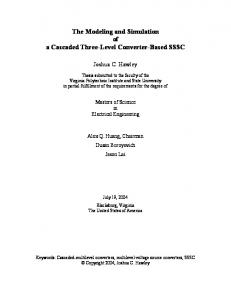
Fig. 4: Schematic plot of a mobile platform equipped with ns steering wheels. the leg extension at a frequency of 250 Hz. Further details on the platform mechanical structure and its onboard electronics can be found in [11]. III. T HE PLATFORM KINEMATIC MODEL In this section, we will consider the kinematic modeling of a platform equipped with several centered steering wheels. The problem will be first addressed for the standard case of fixed legs by borrowing from some of the concepts introduced in [2], [7] and references therein. Goal of this preliminary step is to present and discuss a general methodology for kinematic modeling of fixed-leg platforms. Then, the analysis will be extended to the novel case of movable legs. The developments are kept at the kinematic level by assuming, as usually done, that momentum/inertia of the platform is limited so that dynamics can be neglected, and the actuator velocities can be considered as control inputs. When needed, extensions to dynamic modeling/control are also possible [12], [13]. Hereafter, centered steering wheels (wheels from now on) are modeled as vertical discs able to roll around their horizontal axles, and to rotate around a vertical axis passing through their center (from which the name centered) — see Fig. 3. We also assume that wheels are nondeformable rigid bodies, and that the vertical rods connecting them to the robot chassis are perfectly rigid. Each wheel is supposed to satisfy the perfect rolling constraint, i.e., no longitudinal or lateral slipping during motion. Finally, the platform chassis is also modeled as a perfect rigid body moving on a horizontal plane. A. Case of fixed legs 1) Preliminaries: with reference to Fig. 4, let F0 : {O; X0 , Y0 } be a fixed inertial frame, and FB : {OB ; XB , YB } a moving frame rigidly attached to the platform body. We will denote posture of the platform in F0 the vector ξ = [x y θ]T ∈ R3 , where (x, y) are the coordinates of OB in F0 , and θ the angle between axes XB and X0 . Assume that the platform is equipped with ns independent steering wheels Wi , located at positions Pi in FB , and parameterized by angles φi representing the orientations of

the wheel planes w.r.t. XB . Each wheel is also characterized by two independent velocity inputs taken as control inputs: the linear velocity vWi and the steering velocity vφi = φ˙ i . The configuration of the complete system can be described by the vector q = [ξ T φ1 . . . φns ]T = [ξ T φT ]T ∈ R3+ns , where φ ∈ Rns collects all the ns steering angles. Similarly, we will also adopt the notation vW = [vW1 . . . vWns ]T ∈ Rns and vφ = [φ˙ 1 . . . φ˙ ns ]T ∈ Rns . Due to the assumption of rolling without slipping, each wheel contributes with a Pfaffian first-order constraint in the form [2] − sin(θ + φi )x˙ i + cos(θ + φi )y˙ i = 0, where



xi yi



 =

x y

(1)

 + R(θ)Pi ,

(2)

is the location of wheel Wi in F0 , and R(θ) is the 2 × 2 planar rotation matrix. It can be shown that these constraints are not integrable, i.e., they cannot be reduced to equivalent holonomic constraints and, thus, are denoted as nonholonomic [14]. By combining (2) with (1), we can rearrange the ns nonholonomic constraints in matrix form  − sin(θ + φ ) 1  − sin(θ + φ2 )  ..  . − sin(θ + φns ) 

Ap (q)

0





ξ˙ φ˙

cos(θ + φ1 ) cos(θ + φ2 ) .. . cos(θ + φns )

∆1 ∆2 .. . ∆ ns

 x˙  y˙ 0···0   ˙ θ 0···0   ˙1 .. φ   .  . 0 · · · 0  .. φ˙ ns

     =   

 = A(q)q˙ = 0, (3) ns ×3

with ∆i = Pxi cos(φi ) + Pyi sin(φi ), Ap (q) ∈ R and A(q) ∈ Rns ×(3+ns ) . Equation (3) fully captures the motion restrictions due to the presence of constraints (1). In particular, it follows that a given q˙ is feasible (it satisfies (3)) iff it belongs to the null space of A(q), hereafter denoted as N (q) = N (A(q)). By exploiting the special structure of A(q), and by noting that r = rank Ap (q) ≤ 3, one choice for N (q) is   Np (q) 0 N (q) = 0 Ins where Np (q) = N (Ap (q)) ∈ R3×(3−r) , and In stands for the identity matrix of dimension n. We will then call      ξ˙ Np (q) 0 vp q˙ = = N (q)v = (4) 0 Ins vφ φ˙ the platform kinematic model, where vp ∈ R3−r and vφ ∈ Rns are suitable (pseudo)-velocity inputs that independently affect the platform posture and the steering angles, respectively1 . By construction, this model represents all the possible platform motions q˙ compatible with constraints (3). 1 Here, the physical meaning of v depends on the particular choice for p ˙ Np , while vφ coincides with φ.

Obviously, one is particularly interested in the submodel ξ˙ = Np (q)vp

(5)

which characterizes the planar mobility of the platform, i.e., the possibility to realize an arbitrary linear/angular velocity ˙ Let us then call (5) the posture kinematic model, and ξ. focus on the structure of Np (q). Assume ns ≥ 3 wheels are present in a nondegenerate configuration, i.e., with their centers not all aligned on a same line. Then, in general, rank Ap (q) = 3 and Np (q) = 0 (the trivial null space), implying that no platform motion ξ˙ is possible while satisfying constraints (3). This fact has a well-known geometric explanation (see, e.g., [7]) in terms of the existence of a unique instantaneous center of rotation (ICR) for all wheels. Indeed, validity of Descartes’ principle of motion for rigid bodies implies that all wheel axles must instantaneously meet at a same point on the plane (possibly at infinity) called ICR. Existence of a unique ICR can be seen as a particular geometric (holonomic) constraint requiring the coordination of all wheel orientations. When the ns wheels are in a general configuration, i.e., rank Ap (q) = 3, the ICR constraint is not satisfied and no motion ξ˙ is possible. In order to gain mobility for the platform, we must thus have rank Ap (q) < 3 (existence of a ICR). This implies that at most 2 rows of Ap (q) can be linear independent, say w.l.o.g. the first two associated to wheels W1 and W2 . It can be shown that imposing linear dependency of the remaining ns − 2 rows is equivalent to the following: define the current ICR as the intersection of W1 and W2 axles, and coordinate the remaining ns − 2 wheels such that their axles meet at this ICR [8]. In other words, orientations (φ1 , φ2 ) of wheels W1 and W2 are taken as independent variables, and a set of ns − 2 holonomic constraints φi = hi (φ1 , φ2 ), i = 3 . . . ns , hereafter called coordinating functions, is imposed to coordinate the remaining wheels. Hence (3) becomes  

− sin(θ + φ1 ) − sin(θ + φ2 )

cos(θ + φ1 ) cos(θ + φ2 )

∆1 ∆2

0 0

0 0

    

x˙ y˙ θ˙ ˙ φ1 φ˙ 2

    = 0,   (6)

where now Ap (q) ∈ R2×3 , and one obtains a reduced platform kinematic model      ξ˙ vp  φ˙ 1  = g(q) 0 (7) 0 I v 2

φ˙ 2

φi = hi (φ1 , φ2 ),

φ

i = 3 . . . ns ,

(8)

where only a subset of the original state q appears on the l.h.s. of (7). Here, Np (q) = g(q) ∈ R3 spans the monodimensional null-space of Ap (q) (supposed of rank 2). Note that we assumed vφi = φ˙ i as available inputs for the wheel steering, while the coordinating functions yield the quantity φi . However, the i-th steering velocity can be formally recovered by letting vφi = φ˙ i = h˙ i =

∂hi ˙ ∂hi ˙ φ1 + φ2 . ∂φ1 ∂φ2

(9)

ICR=?

kinematic model

xxxxxxxxxxxxxxxxxxxx xxxxxxxxxxxxxxxxxxxx xxxxxxxxxxxxxxxxxxxx xxxxxxxxxxxxxxxxxxxx xxxxxxxxxxxxxxxxxxxx xxxxxxxxxxxxxxxxxxxx xxxxxxxxxxxxxxxxxxxx xxxxxxxxxxxxxxxxxxxx xxxxxxxxxxxxxxxxxxxx xxxxxxxxxxxxxxxxxxxx xxxxxxxxxxxxxxxxxxxx xxxxxxxxxxxxxxxxxxxx xxxxxxxxxxxxxxxxxxxx xxxxxxxxxxxxxxxxxxxx xxxxxxxxxxxxxxxxxxxx xxxxxxxxxxxxxxxxxxxx xxxxxxxxxxxxxxxxxxxx xxxxxxxxxxxxxxxxxxxx xxxxxxxxxxxxxxxxxxxx xxxxxxxxxxxxxxxxxxxx

W2

xxxxxxxxxxx xxxxxxxxxxx xxxxxxxxxxx xxxxxxxxxxx xxxxxxxxxxx xxxxxxxxxxx xxxxxxxxxxx xxxxxxxxxxx xxxxxxxxxxx xxxxxxxxxxx xxxxxxxxxxx xxxxxxxxxxx xxxxxxxxxxx xxxxxxxxxxx xxxxxxxxxxx xxxxxxxxxxx xxxxxxxxxxx xxxxxxxxxxx xxxxxxxxxxx xxxxxxxxxxx xxxxxxxxxxx xxxxxxxxxxx xxxxxxxxxxx

ξ˙ =

W2

ICR xxxxxxxxxxxxxxxxxxx xxxxxxxxxxxxxxxxxxx xxxxxxxxxxxxxxxxxxx xxxxxxxxxxxxxxxxxxx xxxxxxxxxxxxxxxxxxx xxxxxxxxxxxxxxxxxxx xxxxxxxxxxxxxxxxxxx xxxxxxxxxxxxxxxxxxx xxxxxxxxxxxxxxxxxxx xxxxxxxxxxxxxxxxxxx xxxxxxxxxxxxxxxxxxx xxxxxxxxxxxxxxxxxxx xxxxxxxxxxxxxxxxxxx xxxxxxxxxxxxxxxxxxx xxxxxxxxxxxxxxxxxxx xxxxxxxxxxxxxxxxxxx xxxxxxxxxxxxxxxxxxx xxxxxxxxxxxxxxxxxxx xxxxxxxxxxxxxxxxxxx xxxxxxxxxxxxxxxxxxx

xxxxxxxxxxxxxxxxxxxxxxx xxxxxxxxxxxxxxxxxxxxxxx xxxxxxxxxxxxxxxxxxxxxxx xxxxxxxxxxxxxxxxxxxxxxx xxxxxxxxxxxxxxxxxxxxxxx xxxxxxxxxxxxxxxxxxxxxxx xxxxxxxxxxxxxxxxxxxxxxx xxxxxxxxxxxxxxxxxxxxxxx

W1

xxxxxxxxxxxxxxxxxxxxxxx xxxxxxxxxxxxxxxxxxxxxxx xxxxxxxxxxxxxxxxxxxxxxx

W1

(a)

(b)

Fig. 5: A robot with 2 steering wheels in a nonsingular configuration (left), and in a singular configuration of type B (right).

As for the i-th linear velocity vWi , it can be expressed as a function of vp and the geometry of the platform by simply plugging (7) into (x˙ i , y˙ i ), the time derivative of (2) — see also [7], [8]. Model (7–8) is a valid choice in most situations, but it has two main drawbacks (singularities): A) a coordinating function hi is not defined when the ICR lies exactly on wheel Wi . Indeed, in this situation, any orientation of wheel Wi is compatible with the nonholonomic constraints (the robot is pivoting around Wi ); B) a coordinating function hi is not defined when φ1 = φ2 = arctan(P2x − P1x )/(P1y − P2y ), i.e., when the axles of W1 and W2 are superimposed. In this case, no univocal ICR can be obtained from their intersection. Singularities of type A are, in some sense, ‘structural’. When wheel Wi is at rest, any orientation meets the perfect rolling constraint, so that no φi can be univocally defined. Moreover, from a practical point of view, if the ICR moves arbitrarily close to Wi , the steering velocity φ˙ i grows unbounded, and one should always keeps away from this situation [7]. Therefore, we now focus on the characterization of singularities of type B. For the sake of illustration, we will consider a robot with only 2 steering wheels, and highlight any consideration that does not automatically extend to the general case. Figure 5 depicts such a robot. When singularity B is met (Fig. 5(b)), the ICR can lie everywhere on the common axle of W1 and W2 , i.e., it is not univocally defined. If the robot had more than 2 wheels (not all aligned), one could keep selecting different pairs of wheels not in singularity, and use them to define the ICR [8]. Such a switching strategy can solve the problem of defining functions hi in the general case, but clearly it does not apply to a robot with only 2 wheels. Furthermore, rank of Ap (q) in (6) discontinuously drops to 1 when in singularity B — the two rows of Ap (q) become linear dependent. In particular, it is φ2 ≡ φ1 ≡ const, and (6) reduces to  

− sin(θ + φ1 )

cos(θ + φ1 )

∆



 x˙  y˙  = 0. θ˙

(10)

The platform kinematic model collapses on the posture



g1 (q) g2 (q)



vp

(11)

where now two vectors g1 (q), g2 (q) ∈ R3 span the null space of the (monodimensional) Ap . Note the structural difference between (11) and (7). Obviously, having a kinematic model with a discontinuous structure is not desirable for control design purposes. 2) A general kinematic model: with this in mind, we now propose a general modeling approach that can overcome the difficulties posed by singularities B for a robot equipped with ns > 2 wheels, as well as for the special case ns = 2. All the subsequent developments will be based on this step. The idea is to look at the problem form a different point of view, that is, letting the ICR be defined by the geometric path ξ(t) followed by the platform rather than by the intersection of the axles of any wheel pair (Wi , Wj ), so that singularities B can be structurally avoided. Consider again the situation in Fig. 5(b) and suppose that a ICR, lying anywhere on the common axle, is given as a function of ξ(t). Consistent orientation of the two wheels can still be defined without ambiguities, e.g., φ1 = φ2 = ±π/2 in the reported example. A difficulty could only appear with a ICR lying exactly on one wheel, but this would be again a singularity of type A which, as discussed before, should be avoided. In order to implement this idea, take the i-th constraint in (3) aTi (q)q˙ = 0, and solve it for φi , obtaining φi = arctan

− sin θx˙ + cos θy˙ + Pix θ˙ ˙ = fi (ξ, ξ). cos θx˙ + sin θy˙ − Piy θ˙

(12)

It can be easily shown that numerator (denominator) of (12) is the y˙ i (x˙ i ) component of wheel Wi absolute velocity in FB when the platform is moving along a trajectory ξ(t). Equation (12) is not defined iff (x˙ i , y˙ i ) = (0, 0), i.e., only if wheel Wi is at rest (singularity A). Now, by using (12), it is possible to ‘eliminate’ the last ns − 1 constraints in (3) and obtain an equivalent formulation   x˙

[ − sin(θ + φ1 ) cos(θ + φ1 ) ∆1

 y˙  0 ]  ˙  = 0 (13) θ φ˙ 1

˙ φi = fi (ξ, ξ),

i = 2 . . . ns ,

(14)

where now Ap has constant rank 1. Then, from (13), one can derive by inspection a reduced platform kinematic model 

 cos(θ + φ1 )  ξ˙  sin(θ + φ1 ) =  0 φ˙ 1 0

P1x sin θ + P1y cos θ −P1x cos θ + P1y sin θ 1 0

  0  v 0  W1  ω 0 vφ1 1 (15)

where input ω represents the angular velocity of the platform. It is worth noting that model (14–15) is affected only by singularities A for any value of ns , included the special case ns = 2. Indeed, no rank loss is possible for Ap in (13) (the rank is always 1), and functions (14) are always defined as

long as the ICR does not lie on a wheel2 . A geometrical interpretation is the following: angle φ1 defines the line where the ICR lies (the axle of W1 ), and the ratio vW1 /ω fixes the distance of the ICR from W1 along this line. The other wheels are coordinated, via (16), such that their axles pass through the ICR. Note that ω is not a ‘physical’ input in the sense of (vW1 , vφ1 ). However, by plugging (15) into (12), and by exploiting (2), one can obtain the equivalent expression φi = arctan

vW1 sin φ1 + ω(Pix − P1x ) vW1 cos φ1 + ω(P1y − Piy )

(16)

that shows how to actually realize a given ω by suitably orienting the steering wheels. Here, again, the numerator/denominator are the components of velocity of Wi . Hence, we can adopt model (15), together with functions (16), as the kinematic model describing a mobile platform equipped with ns ≥ 2 steering wheels, and being affected by the sole singularities of type A. As a final consideration, note also that system (15) is completely nonholonomic and, being driftless, also completely controllable. Indeed, by rewriting (15) as [ξ˙T φ˙ 1 ]T = g1 (q)vW1 + g2 (q)ω + g3 (q)vφ1 , one can check that the accessibility rank condition [15]

wheel. It is then possible to exploit the kinematic modeling framework so far presented. Let us consider again a generic platform as the one shown in Fig. 4. In order to not overburden the analysis, we will assume that the moving direction of each leg coincides with vectors Pi , the extension to the general case is immediate. It is useful to express Pi in polar coordinates Pi = [λi cos(αi ) λi sin(αi )]T , with λi being the i-th leg extension, and αi ≡ const the fixed leg direction. Since we assume a time-varying λi (t), it is natural to consider it as a new state of the system. Thus, the complete state vector becomes qc = [ξ T λT φT ]T ∈ R3+2ns , where λ ∈ Rns collects all the λi . Obviously, all wheels still obey the perfect rolling assumption, i.e., the nonholonomic constraints (1) must hold. Therefore, by using (2), we can rearrange the ns constraints in the compact matrix form  − sin(θ + φ1 ) cos(θ + φ1 ) ∆1 Γ1 · · · 0 0 · · · 0   .. .. .. .. . . . ..   . .. . . . . .  − sin(θ + φns ) cos(θ + φns ) ∆ns 0 · · · Γns 0 · · · 0   ˙   ξ Ap (qc ) Aλ (qc ) 0  λ˙  = A(qc )q˙c = 0, φ˙ 

(17)

rank (g1 g2 g3 [g1 , g2 ]) = 4 is always satisfied, being 4 the dimension of vector [ξ T φ1 ]T . B. Case of movable legs Having established a general methodology for modeling a fixed leg platform, we now focus on the case of movable legs which represents the main objective of the paper. As explained in Sect. II, the mechanical structure of our target platform allows the possibility to extend/rectract the legs along a fixed planar direction (the leg direction) without changing the platform height. Therefore, for modeling purposes, we can consider these legs like planar linear ‘joints’ connecting wheels Wi to the platform chassis. With the aim of obtaining a suitable model, it would seem that the dynamical properties of the platform may now play a significant role. Each wheel exerts a force on its own leg and, through the coupling of the platform body, on all the other legs. This results in a completely coupled and second order system where forces of the wheels are partitioned among all legs depending on the particular configuration. However, it turns out that in our case we can still accept the approximation of a simpler kinematic modeling discussed at the beginning of the Section. Indeed, the high mass of the whole platform (about 150 Kg), compared to the very low friction of the leg extension mechanism, allows discarding any dynamical coupling. Basically, the platform behaves as if each leg is an independent linear joint actuated by its own 2 Alternative formulations structurally similar to (7) are also discussed in [7], [8] for a fixed-leg platform. In our case, the main difference is that, acccording to the notation introduced in [2], we reduce the platform kinematics to (15) which is a model of type (2, 1), whereas (7) is of type (1, 2). This manipulation allows to rule out singularities B from the model design.

 ξ˙ λ˙  = φ˙

where Γi = sin(αi −φi ), and Aλ (qc ) = diag(Γi ) ∈ Rns ×ns . Note that submatrix [Ap (qc ) Aλ (qc )], of size ns × (3 + ns ), always admits a null-space of at least dimension 3 whatever the number of wheels ns . Therefore, there always exists an ˙ λ) ˙ meeting constraints (17) regardless infinity of motions (ξ, of the platform configuration. For instance, when the square matrix Aλ (qc ) is nonsingular (αi 6= φi ), choice λ˙ = ˙ ˙ −A−1 λ Ap ξ satisfies (17) for any posture motion ξ, and in any wheel configuration φ. In other words, the ICR constraint, introduced in the previous Section, and imposing a rank condition on Ap , does not extend to the case of movable legs. The reason is that Descartes’ principle of rigid motion is no longer valid since, strictly speaking, the platform cannot be considered as a rigid body because of the leg extension mechanism. Nevertheless, the modeling approach previously presented can be seamlessly extended to this case. To this end, consider the i-th constraint in (17), and solve it for φi to obtain φi = arctan

− sin θx˙ + cos θy˙ + λi θ˙ + sin αi λ˙ i ˙ λ, λ). ˙ = li (ξ, cos θx˙ + sin θy˙ − λi θ˙ + cos αi λ˙ i (18)

Here, again, numerator and denominator of (18) are the components of wheel Wi velocity in FB , so that the expression is valid as long as Wi is not at rest. Proceeding as before, we can eliminate ns − 1 constraints in (17), and get 

− sin(θ + φ1 )

cos(θ + φ1 )

∆1

Γ1 · · · 0

  ˙  ξ ˙  0 λ =0, (19) φ˙ 1

from which by inspection we may derive a reduced platform

can be dynamically linearized. In particular, it is3

kinematic model  cos(θ + φ ) λ sin(θ + α ) − cos(θ + α ) 1 1 1 1  sin(θ + φ1 ) −λ1 cos(θ + α1 ) − sin(θ + α1 )   0 1 0 ξ˙   0 0 1  λ˙ =  0 0 0 φ˙ 1   .. .. ..  . . . 0 0 0

0 · · · 0 z¨ = H(qe )u + M (qe ), H(qe ) ∈ Rm×m , M (qe ) ∈ Rm , (23) 0 · · · 0   T T m 0 · · · 0  vW1 where u = [η˙ vφ1 ] ∈ R is the new input vector made of  0 · · · 0  ω    the steering velocity vφ1 of wheel W1 , and of p ‘acceleration’   vλ  vφ1 signals driving the p integrators η introduced in the dynamic  Ins extension step. Now, by choosing (20)

˙ λ, λ), ˙ φi = li (ξ,

i = 2 . . . ns

(21)

ns

with vλ ∈ R being the (pseudo)-velocity input associated ˙ and qr = [ξ T λT φ1 ]T ∈ Rnq , nq = to the leg velocity λ, 4 + ns the reduced state dimension. By plugging (20) into (18), one can again obtain an expression for φi analogous to (16) φi = ¯li (qr , vR1 , ω, vλ )

(22)

that shows how to actually realize the ‘virtual’ inputs (ω, vλ ) by a proper orientation of the last ns − 1 wheels. Finally, system (20), like (15), can be easily proven to be completely nonholonomic by checking the global validity of the admissible rank condition. IV. D ESIGN OF A KINEMATIC CONTROL LAW Goal of the control algorithm is to have the platform, represented by model (20), asymptotically track a desired posture trajectory ξ ∗ (t) and, at the same time, a desired leg trajectory λ∗ (t). Many approaches for trajectory tracking control of mobile robots have been proposed in the past years, ranging from local feedbacks based on system linearization to global results exploiting Lyapunov techniques. One interesting possibility is to rely on the so-called dynamic feedback linearization [16], [17], [18]. The idea is to select a suitable output function upon which a dynamic compensator, able to fully linearize the input-state-output dynamics, is designed. When this is possible, the closedloop system becomes equivalent to a set of decoupled chains of integrators. Note that full static linearization would be impossible because of the nonholonomy of (20) [17]. In our case, the chosen output function is vector z(qr ) = [ξ T λT ]T ∈ Rm , m = 3 + ns . In order to design a dynamic feedback compensator, one has to iteratively differentiate output z until any input appears. During this process it may be necessary to extend the state of the system by adding integrators on those inputs appearing too early during the differentiation process. Such integrators will constitute the internal state of the dynamic compensator. If, at some point, the extended state dimension equals the total number of output differentiations, full input-state-output linearization can be obtained. For our goals, it turns out that by differentiating twice z(qr ), and by adding p = 2 + ns integrators η to inputs (vW1 , ω, vλ ) in (20), we obtain an extended state qe = [qrT η T ]T of dimension nq + p = 6 + 2ns against 2m = 6 + 2ns total differentiations. Hence, the original model (20)

u(qe ) = H(qe )−1 (v − M (qe )),

v ∈ Rm ,

(24)

we can transform (23) into an equivalent (linear and decoupled) chain of 2m integrators z¨ = v that can be easily stabilized through input v. Exponential regulation of the trajectory tracking error e(t) = z ∗ (t) − z(t) can be achieved by simply taking v = z¨∗ + KD e˙ + KP e,

KD , KP > 0,

(25)

where z ∗ (t) is assumed to be twice differentiable. By choosing diagonal gain matrices, one finally obtains a linear and decoupled closed-loop behavior for e(t) with arbitrary convergence rate. It is also worth noting that feedback (24– 25) is implementable, i.e., it only depends on measurable quantities. Indeed, η is an internal state, z˙ is obtained through (20), and vector qe is known — (λ, φ1 ) are measured and ξ is reconstructed online form wheel encoder readings (dead reckoning). It should be noted that the decoupling matrix H(qe ) is singular at vW1 = 0. This difficulty is structural for mobile robots [17], and is conceptually equivalent to the singularities of type A discussed in the previous Section. In practice, feedback (24–25) can only track a persistent trajectory, i.e., ∗ such that vW (t) 6= 0, ∀t ≥ 0. Assuming z ∗ (t) meets this 1 requirement, the only difficulty may happen during an initial transient phase. Therefore, we relied on the simple strategy of having a perfect matching condition for the platform at the beginning of the motion, so as to avoid intentional transient phases. To this end 1) the reference trajectory z ∗ (t) is always designed such that z ∗ (t0 ) = z(t0 ) and z˙ ∗ (t0 ) = z(t ˙ 0 ). The latter condition is enforced by properly initializing the compensator states η(t0 ) with the initial reference values η ∗ (t0 ) associated to z ∗ (t); 2) similarly to [7], an initial open-loop phase steers each wheel to the value given by (18) computed on z ∗ (t) (i.e., all wheels are initialized with correct and consistent orientations). Hence, the robot starts exactly on the reference trajectory z ∗ (t) and occurrence of transient phases is limited to the presence of external disturbances or unmodeled robot dynamics. As a final remark, note that relations (22) must be derived w.r.t. time in order to obtain the actual steering velocities vφi as done in (9). Clearly, this results in a function of qe and 3 We omit explicit expressions for lack of space. The computation is, however, straightforward.

6 5 end of motion

5 0 0

5

10

15 20 time [s]

25

30

4

ICR locations

y [m]

0.4 0.2 0 0

5

10

15 20 time [s]

25

30

3 end of rotation

2

0.2

1

0

0

−0.2 0

5

10

15 20 time [s]

25

30

Fig. 6: Behavior of θ∗ (t) (top), θ˙∗ (t) (middle) and θ¨∗ (t) (bottom) over time. Note the continuity of θ¨∗ (t) as required by feedback (24–25). η. ˙ As discussed before, the former quantity is measured (η is the internal state of the compensator), while the latter is the output of feedback (24–25). V. E XPERIMENTAL RESULTS In this Section we present the results of an experiment run on the Justin platform described in Sect. II meant to show both the validity of the proposed modeling approach, and the performance of feedbak (24–25). The experiment involves a combined translation/rotation and, at the same time, an extension for the ns = 4 legs. Due to limited space, and also to the difficulty of reporting complex platform motions on a static plot, we omit here results collected on different complex trajectories. A number of these can be appreciated in the video clip attached to the paper. In this simple experiment, the platform starts at ξ(t0 ) = [0 0 0]T with the leg configuration λ(t0 ) = [λm λm λm λm ]T , and must reach ξ(tf ) = [4.5 4.5 2π]T and λ(tf ) = [λM λM λM λM ]T , where λm = 0.37 [m] and λM = 0.56 [m] are the minimum/maximum leg extensions. The chosen reference trajectory z ∗ (t) interpolates component-wise z ∗ (t0 ) with z ∗ (tf ) according to quasi trapezoidal velocity profiles. As a representative case, Fig. 6 depicts the behavior of θ∗ (t) and its derivatives. Note that smooth parabolic arcs replace the constant (but discontinuous) acceleration phases typical for standard trapezoidal profiles, so as to ensure continuity of z¨∗ (t) as required 2 by feedback (24–25). We chose (0.18, 0.1) [m/s, m/s ] ∗ ∗ as maximum velocity/acceleration for both (x (t), y (t)), 2 (0.31, 0.17) [rad/s, rad/s ] for θ∗ (t), and (0.02, 0.01) 2 ∗ [m/s, m/s ] for all λi (t). With these settings, we obtained an overall linear translation lasting tT = 30.8 [s] combined with a rotation ending after tR = 23 [s] and a leg motion ending after tL = 15 [s]. Figure 7 shows the stroboscopic motion of the platform, reconstructed from experimental data, where the different phases are highlighted. Note that maximum velocity/acceleration values for ξ ∗ (t)

end of leg expansion beginning of motion

−1

0

2 x [m]

4

6

Fig. 7: Stroboscopic view of the platform motion during the experiment. Note that the ICR (the small black circle) always lies outside the platform boundaries, and, when the rotation phase is over, goes to infinity. were chosen so that p 2 x˙ ∗ (t) + y˙ ∗2 (t) = R ≥ Rmin = 0.82 [m], |θ˙∗ (t)|

(26)

with R being the instantaneous radius of curvature viewed from the platform center OB and associated to the posture motion ξ ∗ (t). In particular, it is Rmin ≤ R < ∞ for t < tR and R = ∞ for tR ≤ t ≤ tT (during the last phase the platform translates without rotating). Since R also represents the distance between OB and the ICR associated to the posture motion ξ ∗ (t) (see also [7]), we can conclude that trajectory ξ ∗ (t) is free from singularities of type A in the fixed leg case, being Rmin > λM . This fact can also be appreciated in Fig. 7 that shows how the ICR (the small black circle) keeps always outside the platform boundaries. We note, however, that designing ξ ∗ (t) free of singularities is in general not sufficient to ensure definiteness of functions (18) when a leg motion is also present. Indeed, even if the ICR associated to ξ ∗ (t) is ‘properly placed’, a concurrent leg extension/retraction may still result a null linear velocity for some wheels. For instance, if the platform is translating along direction αi of leg i (ICR at infinity), and leg i is expanding with the same velocity but on the opposite direction of motion, wheel Wi must stay exactly at rest and angle φi becomes undefined as in singularities A. Being able to plan in a systematic way a generic trajectory (ξ ∗ (t), λ∗ (t)) free of singularities seems an hard but challenging problem which is, however, beyond the scopes of the present paper. As a first reasonable approximation, we chose to impose very small leg velocities (0.02 [m/s]) so that a quasi-static regime for the platform can be assumed. In this way, the usual ICR constraint can be thought as still valid, and one can simply rely on the planning of ξ ∗ (t) and ‘discard’ the presence of λ∗ (t). In any case, to fully show the possibilities of our approach, the experiments presented in the attached video have been run by also imposing quite higher leg velocities (up to 0.25 [m/s]) and by validating in simulation that no singularity was encountered.

0.4 vW [m/s]

eξ [m]

0.01 0 −0.01 0

5

10

15 time [s]

20

25

30

0.2 0 −0.2 0

5

10

Initial wheel reorientation

15 time [s]

20

15 time [s]

20

25

30

End of platform rotation

−3

x 10

vφ [rad/s]

eλ [m]

5 0

−5 0

5

10

15 time [s]

20

25

30

Fig. 8: Behavior of eξ (t) = ξ ∗ (t) − ξ(t) (top) and eλ (t) = λ∗ (t) − λ(t) (bottom) over time. Note the scales of the plots. Coming back to the design of ξ ∗ (t), condition (26) copes with the presence of singularities of type A. In order to also meet the persistency requirement discussed in the previous Section, we chose to initialize the interpolator with the values |x˙ ∗ (t0 )| = ε, |y˙ ∗ (t0 )| = ε, and |θ˙∗ (t0 )| = ε/Rmin , with ε > 0 being a small threshold tuned experimentally to 0.01 ∗ [m/s]. This guarantees that vW (t0 ) 6= 0, and the correct 1 placement of the ICR during the rest of the motion ensures ∗ that vW (t) 6= 0 ∀ t0 < t < tT . At the end of the trajectory, 1 ∗ (t) → 0, matrix H(qe ) in (24) bewhen t → tT and vW 1 comes ill-conditioned and the tracking performance starts to deteriorate. Therefore, we implemented a simple termination ∗ condition to stop robot motion as soon as |vW (t)| < ε, 1 resulting in a small (but practically negligible) final error e(tT ). This can be verified in Fig. 8 where we show the behavior of e(t) = z ∗ (t) − z(t). One can check that, despite noise, unmodeled dynamics and typical disturbances present in any experiment, feedback (24–25) is fully able to achieve a good tracking (note the scales of the plots) for both the platform posture ξ(t) and the leg configuration λ(t). The control gains chosen for this experiment are KD = 3I7 and KP = 2I7 . In addition, Fig. 9 depicts the behavior of the commanded linear and steering velocities (vW (t), vφ (t)). During an initial phase of about 1 [s], the platform stands still (vW = 0) and the wheels are steered to the nominal values computed from z ∗ (t0 ) and its derivatives. This corresponds to the openloop strategy discussed in point 2 of the previous Section, and meant to correctly initialize the wheel configuration. An horizontal dashed line in the plot marks the end of this preliminary phase and the beginning of the main motion. Note how the velocity commands (in particular vφ (t)) always keep bounded over time, by confirming that no singularity was encountered while executing the motion task. VI. C ONCLUSIONS AND FUTURE DIRECTIONS In this paper, we discussed the kinematic modeling and control problem for a mobile platform equipped with steering wheels and movable legs: the Justin mobile platform. To this end, we first developed a general modeling framework

4 2 0 0

5

10

25

30

Fig. 9: The commanded linear (top) and steering (bottom) velocities to the 4 wheels. The left horizontal dashed line marks the end of the preliminary open-loop phase needed to initialize all wheel orientations, while the right line represents the end of the platform rotation. able to fully capture the peculiarities of this system, that is, variable footprint and omnidirectional capabilities. This was achieved by extending the results obtained for the standard case of a platform with fixed-legs. Then, upon this model, we built a tracking controller capable of realizing arbitrary linear/angular platform motions and independent leg expansion/retraction. The theoretical claims were validated by experimental results that showed good performance of the proposed modeling and feedback approach, and control robustness was also confirmed during the one week operation at the Automatica 2008 fair in Munich. Additional experimental results can be found in the video clip attached to the paper. In the future, we plan to exploit the features of this platform in the complex tasks envisaged for the Justin robot, namely mobile and dexterous two-handed manipulation. In this respect, the proposed controller can be seen as a building block for implementing higher-level modes of operation, such as navigation/exploration or active stabilization during fast motions. ACKNOWLEDGMENTS The authors gratefully acknowledge Prof. Alessandro De Luca, Prof. Giuseppe Oriolo, and Dr. Marilena Vendittelli of the University of Rome “La Sapienza” for useful suggestions. R EFERENCES [1] J. C. Alexander and J. H. Maddocks, “On the kinematics of wheeled mobile robots,” Int. J. of Robotics Research, vol. 8, no. 5, pp. 15–27, 1989. [2] G. Campion, G. Bastin, and B. d’Andr´ea Novel, “Structural properties and classification of kinematic and dynamic models of wheeled mobile robots,” IEEE Trans. on Robotics and Automation, vol. 12, no. 1, pp. 47–62, 1996. [3] P. F. Muir and C. P. Neuman, “Kinematic modeling for feedback control of an omnidiretional wheeled mobile robot,” Proc. of the 1987 IEEE Int. Conf. on Robotics and Automation, pp. 1772–1778, 1987. [4] F. G. Pin and S. M. Killough, “A new family of omnidirectional and holonomic wheeled platforms for mobile robots,” IEEE Trans. on Robotics and Automation, vol. 10, no. 4, pp. 480–489, 1994.

[5] P. F. Muir and C. P. Neuman, “Kinematic modeling of wheeled mobile robots,” J. of Robotic Systems, vol. 4, no. 2, pp. 281–340, 1987. [6] L. Ferri`ere, B. Raucent, and G. Campion, “Design of omnimobile robot wheels,” Proc. of the 1996 IEEE Int. Conf. on Robotics and Automation, pp. 3664–3670, 1996. [7] B. Thuillot, B. d’Andr´ea Novel, and A. Micaelli, “Modeling and feedback control of mobile robots equipped with several steering wheels,” IEEE Trans. on Robotics and Automation, vol. 12, no. 3, pp. 375–390, 1996. [8] A. B´etourn´e and G. Campion, “Kinematic modelling of a class of omnidirectional mobile robots,” Proc. of the 1996 IEEE Int. Conf. on Robotics and Automation, pp. 3631–3636, 1996. [9] E. Jung, H. Y. Lee, J. H. Lee, B.-J. Yi, W. K. Kim, and S. Yuta, “Navigation of an omni-directional mobile robot with active caster wheels,” Proc. of the 2008 IEEE Int. Conf. on Robotics and Automation, pp. 1659–1665, 2008. [10] C. Borst, C. Ott, T. Wimb¨ock, B. Brunner, F. Zacharias, B. B¨auml, U. Hillenbrand, S. Haddadin, A. Albu-Sch¨affer, and G. Hirzinger, “A humanoid upper body system for two-handed manipulation,” Proc. of the 2007 IEEE Int. Conf. on Robotics and Automation, pp. 2766–2767, 2007. [11] M. Fuchs, C. Borst, P. Robuffo Giordano, A. Baumann, E. Kr¨amer, J. Langwald, R. Gruber, N. Seitz, G. Plank, K. Kunze, R. Burger, F. Schmidt, T. Wimb¨ock, and G. Hirzinger, “Rollin’ justin – Design considerations and realization of a mobile platform for a humanoid upper body,” submitted to the 2009 IEEE Int. Conf. on Robotics and Automation, 2009. [12] A. B´etourn´e and G. Campion, “Dynamic modelling and control design of a class of omnidirectional mobile robots,” Proc. of the 1996 IEEE Int. Conf. on Robotics and Automation, pp. 2810–2815, 1996. [13] R. Fierro and F. L. Lewis, “Control of a nonholomic mobile robot: Backstepping kinematics into dynamics,” J. of Robotic Systems, vol. 14, no. 3, pp. 149–163, 1998. [14] J. I. Niemark and N. A. Fufaev, Dynamics of Nonholonomic Systems. Amer. Math. Soc., 1972. [15] A. Isidori, Nonlinear Control Systems, 3rd ed. Springer-Verlag, 1995. [16] B. d’Andr´ea Novel, G. Bastin, and G. Campion, “Dynamic feedback linearization of nonholonomic wheeled mobile robots,” Proc. of the 1992 IEEE Int. Conf. on Robotics and Automation, pp. 2527–2532, 1992. [17] B. d’Andr´ea Novel, G. Campion, and G. Bastin, “Control of nonholonomic wheeled mobile robots by state feedback linearization,” Int. J. of Robotics Research, vol. 14, no. 6, pp. 543–559, 1995. [18] G. Oriolo, A. De Luca, and M. Vendittelli, “WMR control via dynamic feedback linearization: Design, implementation and experimental validation,” IEEE Trans. on Control Systems Technology, vol. 10, no. 6, pp. 835–852, 2002.