PHYSICS OF FLUIDS 25, 071701 (2013)
On the Kolmogorov inertial subrange developing from Richtmyer-Meshkov instability V. K. Tritschler,a) S. Hickel, X. Y. Hu, and N. A. Adams
Institute of Aerodynamics and Fluid Mechanics, Technische Universit¨at M¨unchen, 85747 Garching, Germany (Received 2 April 2013; accepted 27 June 2013; published online 19 July 2013)
We present results of well-resolved direct numerical simulations (DNS) of the turbulent flow evolving from Richtmyer-Meshkov instability (RMI) in a shock-tube with square cross section. The RMI occurs at the interface between a mixture of O2 and N2 (light gas) and SF6 and acetone (heavy gas). The interface between the light and heavy gas is accelerated by a Ma = 1.5 planar shock wave. RMI is triggered by a well-defined multimodal initial disturbance at the interface. The DNS exhibit grid-resolution independent statistical quantities and support the existence of a Kolmogorov-like inertial range with a k−5/3 scaling unlike previous simulations found in the literature. The results are in excellent agreement with the experimental data of Weber et al. [“Turbulent mixing measurements in the Richtmyer-Meshkov instability,” Phys. Fluids 24, C 2013 AIP Publishing LLC. [http://dx.doi.org/10.1063/1.4813608] 074105 (2012)]. !
The Richtmyer-Meshkov instability (RMI) at an interface of two gases has been first investigated by Richtmyer1 and Meshkov.2 It is triggered by the interaction of a shock wave with a material interface. The misalignment of the pressure gradient ∇ p associated with the shock wave and the density gradient ∇ ρ leads to baroclinic vorticity production at the interface between light and heavy gas. The vortex sheet generated between the gases causes the material interface to deform. At very early times, the deformation of the interface can be described by linear theory. However, as soon as the amplitude of the perturbation approaches its characteristic wavelength, the further evolution is dominated by nonlinear effects. The transition from linear to nonlinear growth of the generated vortex sheet is accompanied by Kelvin-Helmholtz instabilities (KHI) at intermediate and late times. The KHI results in a breakup of large-scale structures. Increasingly smaller flow scales are generated until they reach the dissipative and diffusive scaling range, ultimately evolving into a turbulent mixing zone. For a detailed review of the vortex paradigm, see Zabusky.3 Note that also a wave-dynamic paradigm of the RMI evolution has been proposed by Brouillette.4 For the Rayleigh-Taylor instability5 (RTI), it is well known that the initial laminar material interface evolves through the transfer between potential and kinetic energy into a turbulent flow field with a turbulent kinetic energy spectrum. Chertkov6 showed in his work that (in three dimensions) the Kolmogorov-Obukhov theory of steady Navier-Stokes turbulence with a scale independent energy flux can be generalized for Rayleigh-Taylor turbulence in a quasistationary sense. Later, this phenomenological theory was supported by numerical simulations.7–9 The theoretical work of Chertkov6 together with its numerical validation by Boffetta et al.9 led to a coherent and consistent picture of Rayleigh-Taylor turbulence as a Kolmogorov cascade of kinetic energy driven by unstable stratification. Even though the RMI can be considered as the impulsive limit of the RTI, it is lacking such a consistent picture. Zhou10 applied the general framework of Kolmogorov11 and Kraichnan12 to anisotropic and inhomogeneous turbulence evolving from RTI and RMI. The generalization of "1/2 ! Zhou10 includes the definition of a radial wavenumber k = k 2y + k z2 with x being the direction a)
[email protected]
1070-6631/2013/25(7)/071701/7/$30.00
25, 071701-1
! C 2013 AIP Publishing LLC
Downloaded 19 Jul 2013 to 171.64.117.250. This article is copyrighted as indicated in the abstract. Reuse of AIP content is subject to the terms at: http://pof.aip.org/about/rights_and_permissions
071701-2
Phys. Fluids 25, 071701 (2013)
Tritschler et al.
of the shock wave or, in the case of RTI, the direction of gravity. The same radial wavenumber is used in the present study. In his theoretical work, Zhou10 stressed that the spectrum of RichtmyerMeshkov turbulence should scale with k−3/2 as long as the external time scale of the RMI τ RM is much smaller than the time scale of the energy transfer resulting from nonlinear interaction τ nl , i.e., τ RM # τ nl . However, long after shock passage and in the absence of any external agents fully developed turbulence evolving from RMI should recover classical Kolmogorov scaling. Thornber et al.13, 14 found in their multicomponent Euler simulations a Kolmogorov scaling at earlier times that develops towards a k−3/2 range for lower wavenumbers and a Kolmogorov scaling for high wavenumbers at late times. They also found a k−2 scaling as well as a classical Kolmogorov scaling after re-shock depending on the initial condition. Hill et al.15 and Lombardini et al.16 were able to verify the k−5/3 scaling by implicit large-eddy simulations at finite Reynolds numbers. However, the authors did not verify that their result is independent of grid resolution. Cohen et al.17 and Grinstein et al.18 neglected viscous effects and found neither a k−5/3 nor a k−3/2 spectrum range. The wide range of scaling laws observed in numerical simulations is subject to controversial discussions. However, recently published experimental data of Weber et al.19 suggest that a Kolmogorov inertial subrange followed by an exponential decay of the spectrum at higher wavenumbers exists. Hill et al.15 found a k−5/3 spectral range, however, they could not identify a region with an exponential decay beyond the inertial range. In this paper, for the first time grid independent direct numerical simulations (DNS) results are presented. We verify that our simulations qualify as DNS from the facts that (i) energy spectra are resolved well into the dissipative range, (ii) further increase of grid resolution leaves the resolved scale range unchanged and just extends the represented part of the dissipative range, and (iii) the cut-off wavenumber has the same order of magnitude as the Kolmogorov scale. Our data exhibit a Kolmogorov inertial range with a k−5/3 scaling followed by a region of exponential decay. The spectral results thus clearly support the findings of Weber et al.19 and are in excellent agreement with their experimental data up to the highest resolved wavenumbers. We solve the compressible multicomponent Navier-Stokes equations for a mixture of ideal gases with additional transport equations for the species O2 , N2 , SF6 , and acetone. The model for the molecular transport properties of the species includes heat conduction and interdiffusional enthalpy flux.20 The hyperbolic part of the Navier-Stokes equations is solved in characteristic form using Roe’s approximate Riemann solver. For this purpose, the full system including transport equation for the four species is diagonalized. An entropy fix is implemented by Lax-Friedrichs flux splitting, see, e.g., Toro.21 Fluxes are reconstructed in characteristic space by an adaptive central-upwind 6th-order accurate weighted essentially non-oscillatory (WENO-CU6) scheme22 in the low-dissipation version of Hu and Adams.23 Additionally, a positivity-preserving flux limiter24 is employed in order to maintain positive density and pressure. Note that the flux limiter is only active in regions with very high temperature (or low pressure and/or low density) and does not affect the overall accuracy of the 6th-order accurate WENO scheme. It has been verified that it has negligible effect on the results but helps to avoid excessively small time steps that may result due to the stability limit of the explicit time-integration scheme. The WENO-CU6 scheme has already been tested extensively and validated for similar flows.25 The material interface between light and heavy gas is accelerated by a Ma = 1.5 shock wave. In this study, the light gas is considered as a mixture of N2 and O2 with the ratio (in terms of volume fraction) 79:21. The heavy gas is a mixture of SF6 and acetone with mass fractions YSF6 = 0.8 and YAc = 0.2. We use a generic initial multimode perturbation of the interface that is meant to resemble a stochastic perturbation, however, avoiding usage of random numbers that may be hard to reproduce upon changing computing environments. The perturbation of the interface is given by the following function d(y, z) = a1 sin(k0 y) sin(k0 z) + a2
13 # 15 #
n=1 m=3
an,m sin(kn y + φn ) sin(km z + χm )
(1)
Downloaded 19 Jul 2013 to 171.64.117.250. This article is copyrighted as indicated in the abstract. Reuse of AIP content is subject to the terms at: http://pof.aip.org/about/rights_and_permissions
071701-3
Phys. Fluids 25, 071701 (2013)
Tritschler et al.
with a1 = −0.0025 m and a2 = 0.00025 m. The wavenumbers are defined by k0 = 10π /Lyz , kn = 2π n/Lyz , and km = 2π m/Lyz with Lyz being the cross sectional domain size. The amplitudes an, m and the phases φ n , χ m are given by an,m = sin(nm)/2,
(2)
φn = tan(n),
(3)
χm = tan(m).
(4)
The initial position of the interface is at x − d(y, z) = 0. In order to allow for verifying grid convergence, an initial length scale needs to be imposed by prescribing a finite initial interface thickness. The initial material interface thickness results from a smooth description %% $ $ x − d(y, z) 1 (5) 1 + tanh ψ(x, y, z) = 2 Lρ
with L ρ = 0.01 m being the characteristic initial thickness. The lateral widths of the domain are chosen as L y = L z = L yz = 0.1 m. In the x-direction, the domain extends from x = −0.1 m to x = 0.4 m. In this study, three different grid resolutions with cubic cells are considered: a coarse grid with Ny = Nz = 64 cells in the lateral directions, a medium-resolution grid with Ny = Nz = 128, and finally a fine-resolution grid with Ny = Nz = 256 cells. The fine grid results in cubic cells of size 'xyz ≈ 390 µm. For the calculation of the spectra in the inner mixing layer, we define a mixing measure ( by ' & (6) ((x) = 4φ(x) [1 − φ(x)] , with φ(x) = Y S F6 + Y Ac ,
where % · & denotes ensemble averaging in the cross stream planes. A value of ( = 1 corresponds to a fully mixed composition. For the calculation of the radial spectra, we require that ( ≥ 0.9 and average (after the Fourier transform) over all planes that satisfy this condition. Following Moin and Mahesh,26 a simulation qualifies as DNS when dissipation is captured. It is not necessary to resolve the full dissipation range. The smallest resolved length scale can be more than one order of magnitude larger than the Kolmogorov scale η. Here, the Kolmogorov scale can be deduced from a radial Taylor-scale Reynolds number estimate in the inner mixing layer √ Reλ = u r( λ/ν, with ν being the mixture kinematic viscosity for ( = 1 and u r( = u (2y +u (2z being the radial√velocity fluctuations. The Taylor scale λ follows from the turbulent kinetic energy spectra λ = 10ν K /ε with # #1 ˆ k), ˜ ˜ = Rˆ ii (k) E( (7) K = 2 ˜ ˜ k
ε=
$
k
2π L yz
%2 # k˜
1 ˜ = 2ν k˜ 2 Rˆ ii (k) 2
$
2π L yz
%2 #
ˆ k), ˜ 2ν k˜ 2 E(
(8)
k˜
! " ˆ k) ˜ is the kinetic energy of the Fourier mode k˜ = k L yz /2π and Rˆ ii = uˆ (∗ (k) ˜ uˆ ( (k). ˜ An where E( i i estimate for the Taylor-scale Reynolds number in the inner mixing layer then follows Reλ ≈ 369, which is in good agreement with Lombardini et al.16 Taylor scale and Kolmogorov scale are related by $ %1/4 3 λ (10Reλ )1/2 ≈ 38, = (9) η 20
so that, following Pope,27 the Kolmogorov scale is estimated as η ≈ 75 µm. Note that the above estimates, strictly speaking, presume isotropy and incompressibility, that do not hold for evolution times up to about t = 2 ms. In fact, there are clear indications that the estimated Reλ ≈ 369 is too large, as a significantly larger inertial range would occur than observed in the experiments and in computations. An overestimation of Reλ implies an underestimated η, so that the isotropic estimate used for assessing DNS grid resolution requirements results in a significant safety
Downloaded 19 Jul 2013 to 171.64.117.250. This article is copyrighted as indicated in the abstract. Reuse of AIP content is subject to the terms at: http://pof.aip.org/about/rights_and_permissions
071701-4
Tritschler et al.
Phys. Fluids 25, 071701 (2013)
margin. Alternatively, the Kolmogorov scale η can be identified as the particular value that minimizes the deviation of the exponential model spectrum (cη = 0) from our spectra. The characteristic length scale of the largest eddies L = K3/2 /- is calculated from Eqs. (7) and (8), resulting in the estimate η ≈ 224 µm. Thus, it is plausible that the exact Kolmogorov scale is bounded between 75 µm ≤ η ≤ 224 µm. The fine mesh of our simulations resolves smallest scales down to 125 µm for kmax η = 1. Given the estimation ranges for η our fine-mesh simulation clearly qualifies as DNS.26 Weber et al.19 give an estimate for the Batchelor scale λB based on their experimental data, which is the smallest length scale in turbulent passive-scalar mixing. For Sc ≈ 1, the Kolmogorov scale is η ≈ λB .28 Based on Pope’s27 three-dimensional model spectrum for the turbulence kinetic energy and their experimental data, the authors estimate the Batchelor scale in their experiment to 125 µm ≤ λB ≤ 214 µm. This estimate gives a lower-bound for the resolution requirement of π λB ≈ 393 µm in order to resolve the smallest scales. This length scale is one order of magnitude larger than the Reynolds number based estimate λB = CδRe−3/4 Sc−1/2 , where C is a weakly flow dependent constant of order unity, cf. Pope27 and Dimotakis.29 Re is an integral Reynolds number with δ being an estimate for the integral scale, i.e., an appropriately defined mixing layer width. With this paper we provide evidence that in previous investigations the effective Reynolds number was overestimated, and that resolved direct simulations of RMI flows, even with re-shock, at moderate Mach numbers are feasible. Accordingly, the effect of viscosity was considerably underestimated in many Richtmyer-Meshkov investigations that solved only the Euler equations13, 14, 17, 18 or solved the Euler equations and additionally neglected compressibility effects30–32 assuming a constant ratio of specific heats for all fluids involved. Fig. 1 shows the radial power spectra of the density and the radial spectra of the total kinetic energy averaged in the streamwise direction at two different times t = 0.5 ms and t = 2 ms.
FIG. 1. Radial power spectra of the density (a) and radial spectra of the total kinetic energy (b) averaged in the longitudinal (shock propagating) flow direction.
Downloaded 19 Jul 2013 to 171.64.117.250. This article is copyrighted as indicated in the abstract. Reuse of AIP content is subject to the terms at: http://pof.aip.org/about/rights_and_permissions
071701-5
Tritschler et al.
Phys. Fluids 25, 071701 (2013)
Both quantities exhibit grid independence between the medium-resolution grid with 128 cells and the fine grid with 256 cells in the lateral directions, determined from the fact that increasing grid resolution does not affect the respective resolved-scale spectra. At the early times, the dominant initial perturbation is clearly visible. As time proceeds, the generated vortex sheet develops more and more small-scale features. At t = 2 ms, we observe a narrow but distinct Kolmogorov inertial subrange. Despite the existence of the inertial subrange, the dominant initial-condition modes persist to late times. The persistence of the initial condition modes accompanied by a mixed turbulent state was also found in the experimental investigation of Balasubramanian et al.33 We emphasize that the persistence of initial-data large scales and the narrow Kolmogorov inertial range imply an uncertainty about the precise value of the self-similar scaling exponent extracted from the simulation data. Fig. 2 shows contour plots of SF6 mass fraction on the medium and the fine-resolution grid at three different times t = 0.5 ms, 1 ms, and 2 ms. We observe a trend towards a grid converged solution. The large scale structures are identical on the medium and fine grid. However, the fine grid exhibits more small scale features. In the experimental setup of Weber et al.,19 a broadband initial condition is formed by injecting a horizontal shear layer into a vertical shock tube. The broadband spectrum of modes that are present in the experiment can therefore only be described in a statistical sense. Note, that the initial condition in the present numerical investigation is not meant to exactly reproduce the broadband shear layer initial condition of the experiment. However, the comparison between experimental and numerical results given in Fig. 3(a), shows an excellent agreement of spectra. We compare the one-dimensional scalar power spectrum of the experiment with the radial spectrum of the simulation in Fig. 3(a), as one-dimensional spectra follow the same self-similar and dissipative scaling as radial spectra. Both results exhibit an exponential scaling beyond a short inertial range in the power spectrum of the density and the spectrum of the total kinetic energy. From this observation, one can conclude that a Kolmogorov scaling should exist independently of the chosen initial perturbation. However, a remnant of the initial condition at these scales can still be seen at late times despite significantly enhanced small scale features. The compensated radial power spectra of the density given in Fig. 3(b) show a clear emergence of a narrow inertial subrange reflecting the relatively low Taylor-scale Reynolds number of the flow. In Fig. 3(b) also the slopes of the Saffman35, 36 (∼k2 ) and Batchelor34 (∼k4 ) spectra are given. The
FIG. 2. Contour plots of SF6 mass fraction on the medium (a) and the fine-resolution grid (b).
Downloaded 19 Jul 2013 to 171.64.117.250. This article is copyrighted as indicated in the abstract. Reuse of AIP content is subject to the terms at: http://pof.aip.org/about/rights_and_permissions
071701-6
Tritschler et al.
Phys. Fluids 25, 071701 (2013)
FIG. 3. Radial power spectrum of the density and radial spectrum of the total kinetic energy averaged in the longitudinal (shock propagating) flow direction compared to the experiment of Weber et al.19 (a) and the compensated radial power spectra of the density (b) at times t = 0.5 ms and t = 2 ms. Data taken from fine grid DNS.
large scale motion shows a distinct Saffman spectrum E(k) ∼ k2 as k → 0 for all times, independently of resolution. This finding is in contrast to that of Lombardini et al.16 where the authors found that the large scale spectrum, independently of Mach number, deviates from Saffman’s spectrum and instead approaches a Batchelor type spectrum. However, the scaling in the limit of k → 0 may largely depend on the specific initial condition. We can conclude that we have given evidence for the existence of a Kolmogorov inertial subrange independently of the initial perturbation based on grid-converged DNS results. Our numerical results are in excellent agreement with the experimental data of Weber et al.19 The existence of a Kolmogorov inertial range is in contrast to many previously published results where scaling exponents ranging from −2 to −3/2 were observed. From this observation, we conclude that viscous effects have a stronger impact on RMI flows than thought before. For accurate predictions of multifluid mixing, both viscous as well as compressibility effects need to be taken into account. We want to acknowledge that the results in this paper have been achieved using the computing resource SuperMUC based at the Leibniz-Rechenzentrum (LRZ) in Munich, Germany. V.K.T. also wants to acknowledge the support he received from the TUM Graduate School. The authors are grateful for inspiring discussions with Chris Weber, LLNL. 1 R.
D. Richtmyer, “Taylor instability in shock acceleration of compressible fluids,” Commun. Pure Appl. Math. 13, 297 (1960). 2 E. E. Meshkov, “Instability of the interface of two gases accelerated by a shock wave,” Fluid Dyn. 4, 151 (1969). 3 N. J. Zabusky, “Vortex paradigm for accelerated inhomogeneous flows: Visiometrics for the Rayleigh-Taylor and RichtmyerMeshkov environments,” Annu. Rev. Fluid Mech. 31, 495 (1999). 4 M. Brouillette, “The Richtmyer-Meshkov instability,” Annu. Rev. Fluid Mech. 34, 445 (2002). 5 G. I. Taylor, “The instability of liquid surfaces when accelerated in a direction perpendicular to their planes,” Proc. R. Soc. London, Ser. A 201, 192 (1950). 6 M. Chertkov, “Phenomenology of Rayleigh-Taylor turbulence,” Phys. Rev. Lett. 91, 115001 (2003). 7 W. H. Cabot and A. Cook, “Reynolds number effects on Rayleigh–Taylor instability with possible implications for type-Ia supernovae,” Nat. Phys. 2, 562 (2006). 8 N. Vladimirova and M. Chertkov, “Self-similarity and universality in Rayleigh–Taylor, Boussinesq turbulence,” Phys. Fluids 21, 015102 (2009). 9 G. Boffetta, A. Mazzino, S. Musacchio, and L. Vozella, “Kolmogorov scaling and intermittency in Rayleigh-Taylor turbulence,” Phys. Rev. E 79, 065301 (2009). 10 Y. Zhou, “A scaling analysis of turbulent flows driven by Rayleigh–Taylor and Richtmyer–Meshkov instabilities,” Phys. Fluids 13, 538 (2001). 11 A. N. Kolmogorov, “The local structure of turbulence in incompressible viscous fluid for very large Reynolds numbers,” Dokl. Akad. Nauk SSSR 30, 301 (1941). 12 R. H. Kraichnan, “Inertial range spectrum of hydromagnetic turbulence,” Phys. Fluids 8, 1385 (1965). 13 B. Thornber, D. Drikakis, D. L. Youngs, and R. J. R. Williams, “Growth of a Richtmyer-Meshkov turbulent layer after reshock,” Phys. Fluids 23, 095107 (2011).
Downloaded 19 Jul 2013 to 171.64.117.250. This article is copyrighted as indicated in the abstract. Reuse of AIP content is subject to the terms at: http://pof.aip.org/about/rights_and_permissions
071701-7
Tritschler et al.
Phys. Fluids 25, 071701 (2013)
14 B.
Thornber, D. Drikakis, D. L. Youngs, and R. J. R. Williams, “The influence of initial conditions on turbulent mixing due to Richtmyer–Meshkov instability,” J. Fluid Mech. 654, 99 (2010). 15 D. J. Hill, C. Pantano, and D. I. Pullin, “Large-eddy simulation and multiscale modelling of a Richtmyer–Meshkov instability with reshock,” J. Fluid Mech. 557, 29 (2006). 16 M. Lombardini, D. I. Pullin, and D. I. Meiron, “Transition to turbulence in shock-driven mixing: A Mach number study,” J. Fluid Mech. 690, 203 (2012). 17 R. H. Cohen, W. P. Dannevik, A. M. Dimits, D. E. Eliason, A. A. Mirin, Y. Zhou, D. H. Porter, and P. R. Woodward, “Three-dimensional simulation of a Richtmyer–Meshkov instability with a two-scale initial perturbation,” Phys. Fluids 14, 3692 (2002). 18 F. F. Grinstein, A. A. Gowardhan, and A. J. Wachtor, “Simulations of Richtmyer–Meshkov instabilities in planar shock-tube experiments,” Phys. Fluids 23, 034106 (2011). 19 C. Weber, N. Haehn, J. Oakley, D. Rothamer, and R. Bonazza, “Turbulent mixing measurements in the Richtmyer-Meshkov instability,” Phys. Fluids 24, 074105 (2012). 20 A. W. Cook, “Enthalpy diffusion in multicomponent flows,” Phys. Fluids 21, 055109 (2009). 21 E. F. Toro, Riemann Solvers and Numerical Methods for Fluid Dynamics (Springer-Verlag, Berlin, 1999). 22 X. Y. Hu, Q. Wang, and N. A. Adams, “An adaptive central-upwind weighted essentially non-oscillatory scheme,” J. Comput. Phys. 229, 8952 (2010). 23 X. Y. Hu and N. A. Adams, “Scale separation for implicit large eddy simulation,” J. Comput. Phys. 230, 7240 (2011). 24 X. Y. Hu, N. A. Adams, and C.-W. Shu, “Positivity-preserving method for high-order conservative schemes solving compressible Euler equations,” J. Comput. Phys. 242, 169 (2013). 25 V. K. Tritschler, X. Y. Hu, S. Hickel, and N. A. Adams, “Numerical simulation of a Richtmyer-Meshkov instability with an adaptive central-upwind 6th-order WENO scheme,” Phys. Scr. (to be published). 26 P. Moin and K. Mahesh, “Direct numerical simulation: A tool in turbulence research,” Annu. Rev. Fluid Mech. 30, 539 (1998). 27 S. B. Pope, Turbulent Flows (Cambridge University Press, Cambridge, 2000). 28 G. K. Batchelor, “Small-scale variation of convected quantities like temperature in turbulent fluid. Part 1. General discussion and the case of small conductivity,” J. Fluid Mech. 5, 113 (1958). 29 P. E. Dimotakis, “Turbulent mixing,” Annu. Rev. Fluid Mech. 37, 329 (2005). 30 M. Latini, O. Schilling, and W. S. Don, “High-resolution simulations and modeling of reshocked single-mode RichtmyerMeshkov instability: Comparison to experimental data and to amplitude growth model predictions,” Phys. Fluids 19, 024104 (2007). 31 M. Latini, O. Schilling, and W. S. Don, “Effects of WENO flux reconstruction order and spatial resolution on reshocked two-dimensional Richtmyer–Meshkov instability,” J. Comput. Phys. 221, 805 (2007). 32 O. Schilling, M. Latini, and W. S. Don, “Physics of reshock and mixing in single-mode Richtmyer-Meshkov instability,” Phys. Rev. E 76, 1 (2007). 33 S. Balasubramanian, G. C. Orlicz, K. P. Prestridge, and B. J. Balakumar, “Experimental study of initial condition dependence on Richtmyer-Meshkov instability in the presence of reshock,” Phys. Fluids 24, 034103 (2012). 34 G. K. Batchelor and I. Proudman, “The large-scale structure of homogeneous turbulence,” Philos. Trans. R. Soc. London, Ser. A 248, 369 (1956). 35 P. G. Saffman, “The large-scale structure of homogeneous turbulence,” J. Fluid Mech. 27, 581 (1967). 36 P. G. Saffman, “Note on decay of homogeneous turbulence,” Phys. Fluids 10, 1349 (1967).
Downloaded 19 Jul 2013 to 171.64.117.250. This article is copyrighted as indicated in the abstract. Reuse of AIP content is subject to the terms at: http://pof.aip.org/about/rights_and_permissions