Abstractâ The advent of packet networks has motivated many researchers to study the performance of networks of queues in the last decade or two. However ...
On the Maximal Throughput of Networks with Finite Buffers and its Application to Buffered Crossbars Paolo Giaccone Emilio Leonardi Dipartimento di Elettronica Politecnico di Torino, Italy Abstract— The advent of packet networks has motivated many researchers to study the performance of networks of queues in the last decade or two. However, most of the previous work assumes the availability of infinite queue-size. Instead, in this paper, we study the maximal achievable throughput in a flow-controlled lossless network with finite-queue size. In such networks, throughput depends on the packet scheduling policy utilized. As the main of this paper, we obtain a dynamic scheduling policy that achieves the maximal throughput (equal to the maximal throughput in the presence of infinite queuesize) with a minimal finite queue-size at the internal nodes of the network. Though the performance of the policy is ideal, it is quite complex and hence difficult to implement. This leads us to a design of simpler and possibly implementable policy. We obtain a natural trade-off between throughput and queue-size for this policy. We apply our results to the packet switches with buffered crossbar architecture. We propose a simple, implementable, distributed scheduling policy which provides high throughput in the presence of minimal internal buffer. We also obtain a natural trade-off between throughput, internal speedup and buffer-size providing a switch designer with a gamut of designs. To the best of authors’ knowledge, this is one of the first attempts to study the throughput for general networks with finite queue-size. We believe that our methods are general and can be useful in other contexts.
I. I NTRODUCTION Flow-controlled lossless network architectures (like ATM networks [12], [19] or wormhole routed networks [4], [17], [26]) have failed in the context of Internet. However, such network architectures are still widely prevalent in several other contexts such as storage area networks [34], interconnection networks for parallel computing [13], etc. In this paper, we study the throughput performance of such flow-controlled lossless networks. The seminal work of Tassiulas and Ephremides [31] pioneered the research for studying the maximal throughput of controlled networks (also called constrained queueing systems in [31]) with infinite queue-size. For example, the methods of [31] have been utilized in the context of switching [1], [6], [15], [20], [33], satellite and wireless networks [24], [25], etc. Although these results are quite general, they assume the availability of infinite queue-size at all the nodes of the network. In actual applications, queue-sizes are always finite. This is a major limitation of the results of [31] as well as results known in the network theory in general.
Devavrat Shah CS/EE Department Stanford University, USA
In this paper, motivated to analyze performance of networks in the absence of the assumption of infinite queue-size, we study the maximal achievable throughput in flow-controlled lossless networks with finite queue-sizes at the internal nodes of the network. Only the ingress nodes have infinite-size queues to allow us to define the achievable throughput. Our work can be seen as an extension of the results of [31] in the sense that it gets rid of the assumption of infinite queue-size inside the network. As an application of our results, we evaluate the maximal achievable throughput in the packet switch architecture built around a crossbar with buffered crosspoints. Such packet switches have been of a huge recent interest due to the recent advances in the technology [35]. We propose a novel distributed scheduling policy, called DMWF, which is shown to be stable under admissible i.i.d. Bernoulli traffic if either enough internal buffer is present and/or enough internal speedup is available at the crossbar. In particular, we evaluate the natural tradeoff between throughput, speedup and buffersize. We would like to note that though the contribution of this paper is mainly theoretical, we believe that the results obtained in this paper will be useful in the design of network, in sizing buffers and in the design of scheduling policies. A. Organization In Section II, we introduce the notation and the main assumptions of the paper. Then, we present the known results about the maximal throughput for the network of infinite queue-size in Section II-B. In Section III, we present our main results. Finally, in Section IV, we introduce the buffered crossbar switch architecture and apply our results to obtain distributed scheduling policy for buffered crossbar. The proofs of the theorems are presented in the appendix of the paper. II. S YSTEM MODEL AND NOTATION We consider a network of discrete-time physical queues (or stations), handling J customer flows. Customers belonging to flow j, 1 ≤ j ≤ J, enter the network at a station, receive service at each station along an acyclic path and leave the network. The number of stations (hops) traversed by customers of flow j is hj . We assume that the routing of each flow is deterministic. Figure 1 depicts an example of such network.
0-7803-8968-9/05/$20.00 (c)2005 IEEE
internal queue ingress queue
Fig. 1.
server
Example of flow controlled network with 5 servers and 6 flows.
Customers belonging to the same flow, and stored at the same physical queue, form a virtual queue. The number of virtual queues in a network is denoted by Q. We denote with vq the q-th virtual queue in the network. Let q(j, h), with h = 1, . . . , hj , be the index of the queue traversed by flow j at the h-th hop. Virtual queue vq(j,1) is also called “ingress queue” for flow j. The set of all the flow ingress virtual queues {vq(j,1) , 1 ≤ j ≤ J} is denoted with ΦI , whose cardinality is J since each ingress queue is associated with a flow. The set of all the remaining virtual queues, called “internal queues”, is denoted with ΦM . Note that ΦM includes also “egress queues”, i.e. queues traversed by customers just before leaving the network. We now introduce some mapping functions. f (q) maps queue index q to the index of its corresponding ingress queue (first queue): f (q(j, h)) = q(j, 1); note that f (q) = q if q ∈ ΦI . Function u(q) returns the index of the queue upstream to queue vq and it is defined for all the queues except for the ingress queues: u(q(j, h)) = q(j, h − 1), 2 ≤ h ≤ hj . Function p(q) returns the index of queue downstream to queue vq and it is defined for every queue except the egress queues: p(q(j, h)) = q(j, h+1), 1 ≤ h ≤ hj −1. Function j(q) returns the index of the flow traversing queue vq . Servers are associated with physical queues. A server provides service to customers queued at the logical queues (virtual queues) located at its physical queue according to a service policy. Packets are assumed of fixed length normalized to a time slot. All the servers in the network are synchronized. They start service at the beginning of a time slot. All vectors are, by default, row vectors. Let X(n) = [xq (n)]Q q=1 = [x1 (n) x2 (n) . . . xQ (n)], be the vector whose q-th component xq (n) represents the number of customers present in vq (i.e., its queue length1 ) at the beginning of time n, with n ∈ IN+ . For the sake of easier notation, let xj,h (n) equal to xq(j,h) (n). We suppose the size of all the ingress virtual queues (belonging to ΦI ) to be infinite, whereas we assume all the other virtual queues along the flow paths (belonging to ΦM ) to be of finite size. All the virtual queues traversed by flow j can store up to lj customers. A flow control mechanism inhibits the transmission of packets toward queues which are full, thus preventing buffer overflows. The evolution of the number of customers at vq is described 1 Note that “length” denotes the time-variable queue-occupancy, whereas “size” denotes the fixed maximum allowed queue-occupancy.
by xq (n + 1) = xq (n) + eq (n) − dq (n), where eq (n) represents the number of customers that entered vq (and thus its corresponding physical queue) in time interval (n, n + 1], and dq (n) represents the number of customers departed from vq in time interval (n, n + 1]. E(n) = [eq (n)]Q q=1 is the vector of entrances in virtual queues, and D(n) = [dq (n)]Q q=1 is the vector of departures from virtual queues; let dj,h (n) be defined equal to dq(j,h) (n). Given the network state, X(n), the following service constraints on D(n) express the fact that no services can be provided to empty queues and no queue overflows are allowed (thanks to the flow control mechanism): D(n) ≤ X(n) and D(n)R ≤ L − X(n)
(1)
[lq ]Q q=1
being L = the vector with all the queue sizes (assuming lq = ∞ for q ∈ ΦI ). This is equivalent to say: if queue q is empty (xq (n) = 0) or the downstream queue to q is full (xp(q) (n) = lj(q) ), then no service can be provided to queue q (dq (n) = 0). With this notation, the system evolution equation can be written as: X(n + 1) = X(n) + E(n) − D(n)
(2)
The entrance vector E(n) is sum of two terms: vector A(n) = [aq (n)]Q q=1 , representing the customers arrived at the system from outside the network of queues (we also call them external arrivals), and vector of recirculating customers, who are advancing along their paths inside the network, in time interval (n, n + 1]. Since we assume deterministic routing, let the Q×Q matrix R be the routing matrix, with binary elements Rq1 q2 = 1 iff p(q1 ) = q2 and Rq1 q2 = 0 otherwise. The evolution of virtual queues can be rewritten as: X(n + 1) = X(n) + A(n) − D(n)(I − R)
(3)
where I denotes the identity matrix. We suppose that the external arrival process {A(n) : n ∈ IN+ } is a stationary memoryless process, i.e. A(n) are i.i.d. random vectors with average E(A(n)) = Λ = [λq ]Q q=1 . Note that, since external arrivals are directed only to ingress queues, λq = 0 if q ∈ ΦM . At time slot n the scheduling policy selects the service vector S(n), whose element sq (n) represents the amount of work provided to vq during time slot n; let sj,h (n) = sq(j,h) (n). The departure vector D(n) is related to S(n) according to the following equation: � n � � n � n−1 n � � � � D(t) = S(t) ⇒ D(n) = S(t) − D(t) t=0
t=0
t=0
t=0
In other words, the number of packets served from a queue is given by the amount (approximated to the integer part) of cumulative service provided to the queue. We define the difference between the two quantities by: n n � � S(t) − D(t) ∆(n) =
0-7803-8968-9/05/$20.00 (c)2005 IEEE
t=0
t=0
whose q-th element δq (n) ∈ [0, 1) represents the amount of work provided by the scheduling policy to the head-of-theline packets of vq at the end of time slot n. In this paper we restrict our investigation to the class of dynamic scheduling policies, i.e. those scheduling policies which select S(n) on the only basis of the instantanous network state information without requiring any knowledge on the traffic pattern. In general we assume that the set of possible service vectors S(n) is constrained by a system of linear equations representing the topological interference among services at virtual queues (blocking constraints): S(n)K ≤ T
(4)
Matrix K and vector T describe the blocking constraints in the services. For example, simple topological constraints are those expressing the fact that the sum of services provided in each time slot to all the virtual queues residing at the same physical queue is limited by the server capacity. However we do not exclude additional constraints which relate the behavior � the set of of virtual queues residing at different stations. Let D non-negative S(n) which satisfy the blocking constraints. We � defines a polyhedral convex region. Let D the notice that D � For simplicity of notation, we assume set of all vertices of D. that vectors in D are integer valued. In order to avoid trivial cases, we assume that all vectors γ (q) , with 1 ≤ q ≤ Q, whose elements are all null except the q-th, which is unitary, belongs � in other words, � i.e, γ (q) = [0, 0, 0, · · · 1, 0, 0, 0] ∈ D; to D, every virtual queue in the network can potentially get service without violating the topological constraints. We remind that S(n) must be chosen in such a way that the service constraints defined for D(n) in (1) are not violated. If the scheduling policy is atomic, i.e. packets are transmitted by servers in an ‘atomic’ fashion, without interleaving their transmission with packets residing in other virtual queues, then S(n) is integer valued, and D(n) = S(n) for any n. In this case, X(n) is a DTMC (Discrete Time Markov Chain). In the more general case, (X(n), ∆(n)) is a discrete time Markov process defined on a general state space [21]. In the latter case, let us define the workload vector: Y (n) = X(n) − ∆(n)(I − R) We notice that (X(n), ∆(n)) ⇒ Y (n) is a one to one correspondence. Furthermore, it is easy to verify that Y (n) satisfies the following system evolution equation, derived by (3): Y (n + 1) = Y (n) + A(n) − S(n)(I − R)
(5)
Note that is the scheduling policy is atomic, then X(n) = Y (n) for any n and (5) coincides with (3). Finally, let us introduce the following useful positive convex functional: (k) , 1 ≤ Definition 1: Given a vector Z ∈ IRQ + , Z = (z k ≤ Q), the positive convex functional �Z� is defined as: � � 1 � �Z� = inf α ∈ IR+ : Z ∈ D α
We notice that in the remainder of this paper we will refer to it with the improper term of “norm”; furthermore, the previous functional is coincident with the well-known � Under the �Z� Minkowski convex functional associated to D. � then definition immediately follows that, for any S(n) ∈ D, �S(n)� ≤ 1. If the policy is atomic, it chooses S(n) = D(n) ∈ D. To better understand the meaning of such norm, we evaluate now �I�, where I is the vector with unitary elements, in a simple case. Consider a set of independent servers, each of them able to provide one unit of service per time slot, i.e. � If at most i virtual queues γ (q) , 1 ≤ q ≤ Q, is vertex of D. are located at each server, then �I� = i. Indeed, the service � vector S = I/i belongs to the boundary of D. A. Traffic and System Stability Definitions Definition 2: A stationary traffic pattern is admissible if �Λ(I − R)−1 � < 1. Let ρ = �Λ(I − R)−1 �. For the simplest case in which virtual queues residing at different servers are not topologically interacting, traffic is admissible iff no servers are overloaded; in addition, ρ represents the load of the heaviest loaded server in the network. Definition 3: The system of queues is stable if: lim sup E(�X(n)�) < ∞ n→∞
or equivalently: lim sup E(�Y (n)�) < ∞ n→∞
i.e., the system is positive recurrent. Note that the admissibility of traffic pattern is a necessary condition for the system of queue to be stable as shown in [31]. We say that the system is stable at point Λ if it is stable under every stationary memoryless external arrival processes A(n) with average Λ. Definition 4: We define as stability region the set of points Λ in correspondence of which the system of queues is stable. Definition 5: We say that a system of queues is 1-efficient (or equivalently achieves 100% throughput), if it is stable under any admissible traffic pattern. Definition 6: For any 0 < ρ < 1, we say that the system of queues is ρ-efficient if it is stable under any traffic pattern such that �Λ(I − R)−1 � ≤ ρ. B. Previous work The problem of the definition of the stability region in complex systems of interacting queues under dynamic scheduling policies, has attracted significant attention in the last decade from the research community since the pioneering work [31]. In [31], applying the Lyapunov function methodology, it has been shown that a system of interacting queues whose size is infinite achieve 100% throughput, if atomic max-scalar scheduling policy PM S is applied at each node of the network. According to PM S , at each time slot n the departure vector is selected as follows: D(n) = S(n) = arg max Z(I − R)X(n)T
0-7803-8968-9/05/$20.00 (c)2005 IEEE
Z∈D
(6)
The result in [31] has been generalized and adapted to different application contexts in the last years. As matter of example we just briefly recall some of the related works. In the switching context, several studies have been aimed at the definition of the stability region in Input-Queued (IQ) switching architectures built around a bufferless crossbar: papers [1], [15], [20], [30], [33] have proposed different extensions of PM S , which have been shown to be 1-efficient; stability properties for simpler scheduling policies have been also studied in [6], [14]; in [2], [3], [15], finally, the problem of the definition of the stability region in networks of IQ switches has been considered. In the context of the satellite and wireless networks, generalizations of PM S have been recently proposed and shown to be 1-efficient in [24], [25], [32]. All the previous works, however, have considered system of infinite-size queues. In this paper, for the first time, to the best of our knowledge, we extend the investigation about the stability region in systems and networks of queues of finite size subject to some form of flow control which prevents packet losses. C. Stability criteria The stochastic Lyapunov function is a powerful tool to prove stability (i.e., positive recurrency) of Markovian systems. In this subsection we briefly report one of the main results related to the Lyapunov function methodology, which will be used in the remainder of this paper; we refer the interested reader to [11], and [21], [25] for more details on the extension to general state space Markovian processes. Theorem 1: Let Z(n) be an irreducible Q-dimensional Markov chain (or, general space Markov process), whose elements zl (n), l = 1, 2, . . . , Q are non-negative, i.e., Z(n) ∈ Q INQ + (or, Z(n) ∈ IR+ ). If there exists a non-negative valued Q function {L : IR+ → IR+ } such that: E[L(Z(n + 1)) − L(Z(n)) | Z(n)] < ∞
(7)
and E[L(Z(n + 1)) − L(Z(n)) | Z(n)] < −� lim sup �Z(n)� �Z(n)�→∞
(8)
for some � > 0, then Z(n) is positive recurrent, and lim sup E[�Z(n)�] < ∞ n→∞
Inequality (7) requires that the increments of the Lyapunov function L(Z) are finite on average. The second inequality (8) requires that, for large values of �Z�, the average increment in the Lyapunov function from time n to time n + 1 is negative. The intuition behind this result is that the system must be such that a negative feedback exists, which is able to pull the system toward the empty state, thus making it ergodic. For these reasons, inequality (8) is often referred as the Lyapunov function drift condition. In our case, Z(n) represents the number of packets in the network of queue X(n) or the workload Y (n), whose evolution is given by (3) or (5). It is immediate to verify that
constraint (7) can be always met when all the moments of A(n) are finite; in particular, restricting to quadratic Lyapunov functions, it is sufficient that the second moment of A(n) is finite. III. P ERFORMANCE OF NETWORK OF FINITE QUEUES Here we present our main results. In Section III-A we show that 100% throughput can be obtained in any network of finite, flow controlled interacting queues, for lj ≥ 1. To this end, we define the optimal dynamic scheduling policy P1 . Since policy P1 (i) is not atomic, i.e. servers provide fractional services to packets stored at head of the virtual queues, (ii) requires the servers to coordinate their decisions at each time slot, then its implementability results problematic in several application contexts. In Section III-B we propose the atomic dynamic scheduling policy P2 whose complexity is similar to PM S defined for infinite queue networks. P2 , similarly to PM S , requires a continuous exchange of state information among network servers, but it can allow servers to take local decisions in an uncoordinated fashion, when considering simple network configurations, thus resulting significantly less complex than P1 . We show that P2 is ρ-efficient when enough buffer inside the network is provided, thus estimating the trade-off between network buffers and achievable throughput. A. Optimal policy 1) Policy definition: Consider the following policy, called P1 , in vectorial format: S(n) = arg max Z(I − R)M(n) (2Y (n) − Z(I − R))
T
� Z∈D
(9) where M(n) is a Q × Q matrix, non-null only on its diagonal where, for q = 1, . . . , Q: 1 Mqq (n) = yf (q) (n) lj(q)
if q ∈ ΦI if q ∈ ΦM
We now express the policy in scalar format (for the sake of easier notation, we omit (n) when not necessary). Observe that:
sq if q ∈ ΦI [S(I − R)]q = sq − su(q) if q ∈ ΦM and multiplying by M: [S(I − R)M]q =
sq
yf (q) (sq − su(q) ) lj(q)
if q ∈ ΦI if q ∈ ΦM
Hence, if we define that yp(q) /lj(q) = 0 if queue q is an egress
0-7803-8968-9/05/$20.00 (c)2005 IEEE
queue, the first adder in (9) becomes: f1 (S) = S(I − R)MY T = � � yf (q) sq yq + (sq − su(q) ) = lj(q) q∈ΦI q∈ΦM � � � � yp(q) yq − yp(q) sq yq 1 − sq yf (q) + = lj(q) lj(q) q∈ΦI q∈ΦM hj J � � yj,1 sj,1 (lj − yj,2 ) + sj,h (yj,h − yj,h+1 ) (10) l j=1 j h=2
whereas the second adder in (9): f2 (S) = S(I − R)M[S(I − R)]T = � � � �2 yf (q) sq − su(q) s2q + = lj(q) q∈ΦI
J �
s2j,1 +
J �
j=1
j=1
J �
J �
s2j,1 +
j=1
j=1 J � j=1
s2j,1 +
q∈ΦM
hj yj,1 � 2 (sj,h + s2j,h−1 − 2sj,h sj,h−1 ) = lj h=2
hj yj,1 � 2 (sj,h + s2j,h−1 − 2sj,h sj,h−1 ) = lj h=2
J � j=1
hj −1 � yj,1 � 2 sj,1 + 2 s2j,h + s2j,hj − lj
2
�
� sj,h sj,h+1
(11)
h=1
(12)
� Z∈D
with f (Z) = 2f1 (Z) − f2 (Z). Observe that according to policy P1 , by construction, service is never provided to empty virtual queues, thus satisfying one of the service constraints. This can be easily seen by observing that P1 can be equivalently defined as: S(n) = arg min
�
� Z∈D
[Y (n) − Z(n)(I − R)]M(n)[Y (n) − Z(n)(I − R)]T
1) Policy definition: Consider the following policy, called P2 : S = arg max Z(I − R)MY T � Z∈D
By combining (10) and (11), policy P1 becomes: S = arg max f (Z)
lj ≥ 1 for j = 1, . . . , J 3) Implementation issue: Since P1 is not atomic, it selects � and this does not guarthe best service vector S in the set D antee that S is a integer departure vector; in simpler words, sq ∈ [0, 1]. As a consequence, the direct implementation of policy P1 requires servers to provide fractional services to packets stored at head of the virtual queues according to a weighted processor sharing policy. Moreover, according to policy P1 , packets are transferred through queues in a “cut-through” fashion, since servers may start the transmission of non completely received packets. We notice that non-atomic scheduling policies exploiting “cutthrough” switching have been proposed and implemented in the contexts of wormhole networks [7], [10], [26]. At last, P1 must be implemented in a centralized fashion by a scheduler which has the complete view of the queues state of the network. The high implementation complexity of this policy has motivated our investigation on the performance of the following policy. B. Low complexity policy
h=2
hj −1
Theorem 2: Under admissible Bernoulli traffic, policy P1 achieves 100% throughput when the buffer size lj (not counting the slack buffer) of any internal queue q traversed by flow j satisfies the following relation:
�
and observing that the minimum is always achieved when all the elements of [Y (n) − Z(n)(I − R)] are non negative. The second service constraint, which avoids buffer overflows, is not always precisely met by P1 . However it is easy to realize that according to P1 , Y (n) ≤ L + cI, for all n, being c the maximum amount of service that any server in the network can provide in a time slot. As a conclusion, to avoid buffer overflow is sufficient to provide any virtual queue with an extra amount of memory (called slack-buffer) equal to c. 2) Policy performance: Now we state our main theorem, whose proof is reported in Appendix I.
In other words, policy P2 maximizes the scalar product of the service vector Z and the weight vector W = (I − R)MY T . Due to the linearity of the scalar product, P2 guarantees the � i.e. S(n) ∈ D. Hence, P2 is an vector S to be a vertex of D, atomic policy and X(n) = Y (n). Formally, we can say that P2 can be expressed as: D = arg max Z(I − R)MX T Z∈D
Following the same reasoning to obtain (10), a generic queue q is associated with the following weight wq : � x xq 1 − p(q) if q ∈ ΦI � lj(q) (13) wq = xq − xp(q) if q ∈ ΦM xf (q) lj(q) then policy P2 can be rewritten as: D = arg max Z∈D
Q �
zq wq
(14)
q=1
We define the policy such that dq = 0 when wq = 0; note also that dq = 0 when wq < 0. Hence, policy P2 satisfies the service constraints: if xq = 0 or xp(q) = lj(q) then wq ≤ 0 and then dq = 0 as expected.
0-7803-8968-9/05/$20.00 (c)2005 IEEE
2) Policy performance: We claim the main result about P2 , whose proof is reported in Appendix II. Theorem 3: Under admissible Bernoulli traffic, policy P2 is ρ-efficient when the buffer size lj of any internal queue q traversed by flow j, with hj hops, satisfies the following relation: (hj − 1)�I� for j = 1, . . . , J lj > 2(1 − ρ) recalling that ρ = �Λ(I − R)−1 �, and I is the vector with unitary elements. A special case applies for networks with at most two hops, like the switches built around buffered crossbars and discussed in Section IV. We can claim the following: Corollary 1: Under admissible Bernoulli traffic, for a network with hj ≤ 2 for all j, policy P2 achieves 100% throughput, when ρ < 0.5 for any lj ≥ 1, being ρ the maximum offered load for a single queue in the network. The proof is reported in Appendix III. From this corollary, it results that any choice of lj the network is 0.5-efficient, under the condition that no packet routes are longer than two hops. 3) Implementation issue: Policy P2 is an atomic policy equivalent to PM S of (6), but with different weights assigned to the internal queues. Indeed, P2 and PM S solve the same optimization problem since they both share the same linear structure of the cost function and the same space D of feasible departure vectors. Both policies require a continuous exchange of information between neighbor servers, but in addition P2 requires locally at each server the information about the length of the ingress queue of the corresponding flows. Note that this length should be propagated downstream from the ingress queue to all the internal queues, along the flow path: this fact can be exploited to ease the implementation. In general, given the state of all the queues, P2 is executed by a central scheduler, as also observed by [31]. However, in particular (but also interesting) cases, the policy can be computed in a distributed fashion, locally on each set of queues and servers which are coupled by the blocking constraints. This fact is indeed exploited in the following section to devise a computationally efficient scheduling policy for packet switches. IV. A PPLICATION TO PACKET SWITCHES BASED ON BUFFERED CROSSBARS
Recently, switches built around crosspoint buffered crossbars have been shown to be very promising solutions for the design of fast and scalable switching architectures. A basic model for a switch with internal buffered crossbar is depicted in Fig. 2. To avoid the negative effects of the head-of-theline blocking phenomenon, inputs cards adopts Virtual Output Queue (VOQ) scheme, according to which packets are stored at inputs in per-destination virtual queues. Each crosspoint of the crossbar is provided with an internal buffer of size L: internal buffers are in one-to-one correspondence with input VOQs. We refer to this architecture as
IN 1
IN 2
IN N
OUT 1
Fig. 2.
OUT 2
OUT N
The N × N CICQ architecture with VOQ and buffered crosspoints
Combined Input and Crossbar Queued (CICQ) switch. A flow control mechanism from each crosspoint to the corresponding VOQ avoids to overflow the internal buffer. Assume time to be slotted, and packets to be of fixed size. With respect to pure input queued switches, the scheduling policies in CICQ switches can be simpler. The scheduling decision, indeed, can be taken in a local uncoordinated fashion by an arbiter at each input, selecting a non-full internal buffer to which transferring a packet, and by an arbiter at each output, selecting an internal buffer from which transferring a packet. We refer in the following to this class of schedulers as “uncoordinated schedulers”. Uncoordinated schedulers can be efficiently distributed, parallelized, and pipelined. Mainly for this reason, CICQ switches are widely considered scalable and timely. Note that, in uncoordinated schedulers, we admit that inputs and outputs can exchange some information about the state of the queues, but we assume the scheduling decision to be local. Furthermore, uncoordinated schedulers cannot be implemented in pure IQ switches, since coordination is required at inputs to avoid multiple transmissions toward the same output. Here, we restrict our discussion to uncoordinated schedulers. An overview of the evolution of CICQ switches has been recently proposed in [35], but also [28] provides a wide introduction to CICQ switches. We refer to both cited papers for the main algorithms proposed so far to control the CICQ architecture, aimed at providing high throughput, or supporting QoS or variable size packets [9]. The two main families of input arbiters and output arbiters proposed and studied so far have been the following: •
•
round-robin based: the queue is selected according to a round robin (RR) mechanism [27], [28], [29], or to a weighted round robin (WRR) [5], or to a weighted fair queueing scheme (WFQ) [5]; queue-state based: the queue with largest length (LQF) [8], or the largest waiting time of the HoL cell (OCF) [8], [23], or the largest/shortest internal queue length [22], is selected.
Note that the input arbiters can select a VOQ queue among the
0-7803-8968-9/05/$20.00 (c)2005 IEEE
VOQs which are not inhibited by the flow control mechanism. Unfortunately, so far general theoretical results have been missing about the stability of CICQ for speedup SP < 2. Many papers have addressed the case SP = 1 but proving stability properties only under some ideal traffic scenarios, for example when the arrival rates for each input output port are known (e.g., in the case of uniform traffic). The simplest scheme of CICQ is based on RR-RR (notation is:“input arbiter”“output arbiter”) [27] and L = 1; this scheme has been proved to be stable only for uniform traffic, indeed it has been shown to be unstable when the traffic is non-uniform ([8] and [35]). For the RR-RR scheme it has been shown [28] by simulation that small buffers (L = Θ(N )) cannot be sufficient to provide 100% throughput, unless some moderate speedup is introduced. When adopting LQF-RR and L = 1, the CICQ has been proved to achieve the 100% throughput just when input/output pair loading is ≤ 1/N [8]. Many other variants have been proposed (like in [5], [22], [29], [35]), achieving high throughput under non-uniform scenarios, but their performance has been shown only by simulation. How to dimension L has been discussed by many papers, which have related L only to the round trip time delay dRT T of the flow control mechanism from the internal crosspoint to the input arbiters. In order to sustain a line rate r, L should be set larger coarsely than the product dRT T × r. For SP = 2, perfect emulation of an output queued switch (both FIFO and non-FIFO) [18] can be performed. In other words, SP = 2 is sufficient to achieve 100% throughput, workconservation and perfect delay control under any admissible traffic. The requirement for L is minimal, since it is aimed just at compensating for dRT T . To our best knowledge, no theoretical results are known which prove that CICQs with SP < 2, exploiting uncoordinated schedulers, can achieve 100% throughput under any admissible traffic pattern. Now observe that a CICQ switch can be modeled as a flow controlled network, with one server for each input (corresponding to the input arbiter) and with one server for each output (corresponding to the output arbiter). The flow control is from the internal buffers to the corresponding input arbiters. Hence, we can particularize to this context the general results obtained in the previous section. We restrict our investigation to policy P2 which can be easily implemented in a CICQ as an uncoordinated scheduler. A. Scheduling algorithms for CICQ Let xij be the length of VOQ from input i to output2 j. Let bij be the length of the corresponding internal buffer; 0 ≤ bij ≤ L, and when bij = L the flow control mechanism inhibits the services from the corresponding VOQ: we assume that the flow control is immediate. Departure vector D comprises the services provided by the input arbiters and the output arbiters: dIij describes the departure from the VOQ 2 With abuse of notation, here j stands either for a flow identifier or an output.
corresponding to xij , whereas dO ij describes the departure from the internal buffer corresponding to bij . The set D of all possible departing vectors is given by all D such that N �
dIij ≤ 1
∀i
and
j=1
N �
dO ij ≤ 1
∀j
i=1
which describe the blocking constraints of (4) in the context of a CICQ switch. We particularize the policy P2 by showing that it can be easily implemented in an uncoordinated fashion. Indeed, revisiting (14), P2 selects the departing vector according to: 2
D = arg max D∈D
N � xj,1 j=1
arg max D∈D
L
(dj,1 (L − xj,2 ) + dj,2 xj,2 ) =
N � N �
xij (dIij (L − bij ) + dO ij bij )
(15)
i=1 j=1
Let MWF be the “maximum weight first” policy, which serves the queue with the maximum strictly positive weight. D satisfying (15) can be obtained by: • •
maximizing, for each input i, the product dIij × xij (L − bij ) among all possible j; this is MWF policy; maximizing, for each output j, the product dO ij × xij bij among all possible i; this is again MWF policy.
As a consequence policy P2 operating a CICQs can be redefined as DMWF (Dual Maximum Weight First) according to the following algorithmic description: • • • •
I at each time slot, associate to each VOQ a weight wij = xij (L − bij ); select at each input the non inhibited VOQ which maxiI over all j = 1, . . . , N ; mizes wij at each time slot, associate to each internal buffer a weight O = xij bij ; wij select at each output the non-empty internal buffer which O over all i = 1, . . . , N . maximizes wij
Thanks to corollary 1, DMWF is ρ-efficient if ρ < 0.5 for any L ≥ 1. Note that in the case L = 1, then DMWF degenerates into LQF-LQF scheduler. If we now apply Theorem 3, in a CICQ switch �I� = N since N are the queues conflicting in the same input/output arbiter. Hence, in general L should be set such that L > N/(1 − ρ)/2. To summarize, we can claim the following: Corollary 2: Under admissible admissible Bernoulli traffic, in a CICQ switch policy DMWF is ρ-efficient for L ≥ Lmin with 1 � � if ρ < 0.5 Lmin = N if 0.5 ≤ ρ < 1 2(1 − ρ) where ρ is the maximum offered load to an input and output port of the switch.
0-7803-8968-9/05/$20.00 (c)2005 IEEE
The result of corollary 2 can be restated also as follows: the sustainable load is at least: 0.5 for 1 ≤ L ≤ N ρ= N 1 − for L > N 2L or equivalently: Corollary 3: Under admissible admissible Bernoulli traffic, the minimum speedup to guarantee 100% throughput in a CICQ switch adopting DMWF policy, is 2 for 1 ≤ L ≤ N SP = 2L for L > N 2L − N This proves the existence of a tradeoff between throughput (or speedup needed) and L under DMWF. V. C ONCLUSIONS We have considered a network/system of interacting queues with internal queues of finite size. A flow control mechanism from each queue prevents losses to occur. We devised two stable policies, P1 and P2 , the first achieving 100% throughput and the second ρ-efficient, under Bernoulli i.i.d. traffic. Policy P1 requires to solve a quadraticform optimization problem on the state of workload given to each queue. This policy can be very complex to implement, but requires a minimal amount of one buffer location for each queue. On the contrary, policy P2 is based on the solution of a linear-form optimization problem on the state of occupation of the queues. This policy is very similar to the max-scalar policy proposed in the past for interacting queues with infinite-size buffer, and its computational complexity is lower than P1 . But the requirement on the amount of buffer is larger than P2 . As example of application of our general theoretical results, we have considered a N × N input queued switch built around a buffered crossbar. In this case, P2 degenerates into an uncoordinated scheduling policy, called DMWF, in which each input and output arbiter can choose among N queues on the basis of the highest weight assigned to each queue. We have discussed the minimum buffer requirement for the internal queues, and its tradeoff with the allowed speedup and throughput in the crossbar. R EFERENCES [1] M. Ajmone Marsan, A. Bianco, P. Giaccone, E. Leonardi, F. Neri, “Packet-Mode Scheduling in Input-Queued Cell-Based Switch”, IEEE/ACM Transactions on Networking, vol. 10, n. 5, Oct. 2002, pp. 666-678 [2] M. Ajmone Marsan, P. Giaccone, E. Leonardi, F. Neri, “On the stability of local scheduling policies in networks of packet switches with input queues”, IEEE Journal on Selected Areas in Communications, vol. 21, n. 4, May 2003, pp. 642-655 [3] M. Andrews, L. Zhang, “Achieving Stability in Networks of InputQueued Switches”, IEEE INFOCOM 2001, Anchorage, Alaska, USA, Apr. 2001, pp. 1673-1679 [4] N.J. Boden et al., “Myrinet: a gigabit-per-second local area network”, IEEE Micro, vol. 15, n. 1, Feb. 1995, pp. 29-36 [5] N. Chrysos, M. Katevenis, “Weighted Fairness in Buffered Crossbar Scheduling”, IEEE HPSR 2003, Torino, Italy, June 2003, pp. 17-22 [6] J.G. Dai, B. Prabhakar, “The throughput of data switches with and without speedup”, IEEE INFOCOM 2000, Tel Aviv, Israel, Mar. 2000, pp. 556-564
[7] J. Duato, “A necessary and sufficient condition for deadlock-free adaptive routing in wormhole networks”, IEEE Trans. on Parallel and Distributed Systems, vol. 6, n. 10, Oct. 1995, pp. 1055-1067 [8] T. Javadi, R. Magill, T. Hrabik, “A high throughput scheduling algorithm for a buffered crossbar switch fabric”, IEEE ICC 2001, June 2001, pp. 1581-1591 [9] M. Katevenis, G. Passas, D. Simos, I. Papaefstathiou, N. Chrysos, “Variable Packet Size Buffered Crossbar (CICQ) Switches”, IEEE ICC 2004, Paris, France, June 2004 [10] P. Kermani, L. Kleinrock, “Virtual Cut-through: A New Computer Communication Switching Technique”, Computer Networks, vol. 3, n. 3, Sep. 1979, pp. 267-286 [11] P.R. Kumar, S.P. Meyn, “Stability of Queueing Networks and Scheduling Policies”, IEEE Trans. on Automatic Control, vol. 40, n. 2, Feb. 1995, pp. 251-260 [12] H.T. Kung, K. Chang “Receiver-oriented adaptive buffer allocation in credit-based flow control for ATM networks” IEEE INFOCOM ’95, Boston, MA, USA, Apr. 1995, pp. 239-252 [13] F.T. Leighton, Introduction to Parallel Algorithms and Architectures: Arrays, Trees and Hypercubes, Morgan Kaufmann, 1991 [14] E. Leonardi, M. Mellia, F. Neri, M. Ajmone Marsan, “On the Stability of Input-Queued Switches with Speedup”, IEEE/ACM Trans. on Networking, vol. 9, n. 1, Feb. 2001, pp. 104-118 [15] E. Leonardi, M. Mellia, M. Ajmone Marsan, F. Neri, “On the Throughput Achievable by Isolated and Interconnected Input-Queueing Switches under Multiclass Traffic”, IEEE INFOCOM 2002, New York, NY, USA, June 2002 [16] E. Leonardi, M. Mellia, F. Neri, M. Ajmone Marsan, “Bounds on Average Delays and Queue Length Averages and Variances in Input Queued and Combined Input/Output Queued Cell-Based Switches”, Journal of the ACM, vol. 50, n. 4, July 2003 [17] X. Lin, P.K. McKinley, L.M. Ni, “The message flow model for routing in wormhole-routed networks”, IEEE Trans. on Parallel and Distributed Systems, vol. 6, n. 7, July 1995, pp. 755-760 [18] R.B. Magill, C.E. Rohrs, R.L. Stevenson, “Output queued switch emulation by fabrics with limited memory”, IEEE Journal on Selected Area in Communications, vol. 21, n. 4, May 2003 [19] S. Mascolo, D. Cavendish, M. Gerla, “ATM rate based congestion control using a Smith predictor: an EPRCA implementation”, IEEE INFOCOM ’96, San Francisco, CA, USA, Mar. 1996, pp. 569-576 [20] N. McKeown, A. Mekkittikul, V. Anantharam, J. Walrand, “Achieving 100% throughput in an input-queued switch”, IEEE Trans. on Communications, vol. 47, n. 8, Aug. 1999, pp. 1260-1272 [21] S.P. Meyn, R. Tweedie, Markov Chain and Stochastic Stability, SpringerVerlag, 1993 [22] L. Mhamdi, M. Hamdi, “MCBF: a high-performance scheduling algorithm for buffered crossbar switches”, IEEE Communications Letters, vol. 7, n. 9, Sept. 2003, pp. 451-453 [23] M. Nabeshima, “Performance evaluation of a combined input and crosspoint queued switch”, IEICE Trans. Comm., vol. E83-B, n. 3, Mar. 2000 [24] M.J. Neely, E. Modiano, C.E. Rohrs, “Dynamic power allocation and routing for time varying wireless networks”, IEEE INFOCOM 2003, vol. 1, Mar. 2003, pp. 745-755 [25] M.L. Neely, E. Modiano, C.E. Rohrs “Power Allocation and Routing in Multibeam Satellites with Time-Varying Channels”, IEEE/ACM Trans. on Networking, vol. 11, n. 1, Feb. 2003, pp. 138-152 [26] L.M. Ni, P.K. McKinley, “A survey of wormhole routing techniques in direct networks” IEEE Computer, vol. 26, n. 2, Feb. 1993, pp. 62-76 [27] R. Rojas Cessa, E. Oki, Z. Jing, H.J. Chao, “CIXB-1: combined inputone-cell-crosspoint buffered switch”, IEEE HPSR 2001, Dallas, USA, pp. 324-329 [28] R. Rojas Cessa, E. Oki, H.J. Chao, “CIXOB-k: combined inputcrosspoint-output buffered packet switch”, IEEE GLOBECOM 2001, Nov. 2001, pp. 2654-60 [29] R. Rojas-Cessa, E. Oki, “Round robin selection with adaptable size frame in a combined input-crosspoint buffered switch”, IEEE Communications Letters, vol. 7, n. 11, Nov. 2003 [30] K. Ross, N. Bambos, “Local Search Scheduling Algorithms for Maximal Throughput in Packet Switches”, IEEE INFOCOM 2004, Mar. 2004 [31] L. Tassiulas, A. Ephremides, “Stability properties of constrained queueing systems and scheduling policies for maximum throughput in multihop radio networks”, IEEE Trans. on Automatic Control, vol. 37, n. 12, Dec. 1992, pp. 1936-1948
0-7803-8968-9/05/$20.00 (c)2005 IEEE
[32] L. Tassiulas, “Scheduling and performance limits of networks with constantly changing topology”, IEEE Transactions on Information Theory, vol. 43, n. 3, May 1997, pp. 1067-1073 [33] L. Tassiulas, “Linear complexity algorithms for maximum throughput in radio networks and input queued switches”, IEEE INFOCOM 1998, San Francisco, CA, USA, Apr. 1998 [34] R. Telikepalli, T. Drwiega, J. Yan, “Storage area network extension solutions and their performance assessment”, IEEE Communications Magazine, vol. 42, n. 4, April 2004, pp. 56-63 [35] K. Yoshigoe, K.J. Christensen, “An evolution to crossbar switches with virtual output queueing and buffered crosspoint”, IEEE Network, Sept. 2003, pp. 48-56
A PPENDIX I P ROOF OF THEOREM 2 Proof: Consider the following Lyapunov3 function: L(Y (n)) = Y (n)M(n)Y T (n). If ∆L(n) = E[L(Y (n+1))− L(Y (n))|Y (n)], the stability criteria of (8) becomes: lim
�Y (n)�→∞
∆L(n) < −� �Y (n)�
(16)
where
[A(n) − S(n)(I − R)]M(n + 1)[A(n) − S(n)(I − R)]T − � (17) Y (n)M(n)Y (n)T Now observe the M(n + 1) = M(n) + o(�Y �) when �Y � → ∞, since |yf (q) (n + 1) − yf (q) (n)| ≤ 1. Hence, we can substitute M(n + 1) with M(n) and obtain: ∆L(n) = � � E 2[A(n) − S(n)(I − R)]M(n)Y T (n) + � E A(n) − S(n)(I − R)]M(n) � [A(n) − S(n)(I − R)]T = � � 2E [Λ − S(n)(I − R)]M(n)Y T (n) +
λq − λp(q) = λq [(I − R)Λ ]q = 0
3 Note
if q ∈ ΦI if q ∈ ΦM
∆L ≈ 2ΛMY T − 2f1 (S) + f2 (S)
(20)
If we now define Γ = Λ(I−R)−1 , then ΛMY T can be written as f1 (Γ). Since Λ is admissible it results: �Γ� = ρ < 1; we ˆ such that Γ = ρΓ: ˆ �Γ� ˆ = 1 and Γ ∈ D. can now define Γ ˆ = ρf1 (Γ). ˆ Since f1 is a linear function, then f1 (Γ) = f1 (ρΓ) −1 −1 T ˆ Now 2ρf2 (Γ) = 2ρ f2 (Γ) = 2ρ ΛMΛ is o(�Y �) and can be substracted from (20): ˆ − f (S) ≈ ∆L ≈ 2f1 (Γ) − f (S) = 2ρf1 (Γ) ˆ − 2ρf2 (Γ) ˆ − f (S) = ρf (Γ) ˆ − f (S) 2ρf1 (Γ) ˆ Now, considering the definition of policy P1 , f (S) ≥ f (Γ) and we can say: (21)
J � 2 2 � 2 ˆ ˆ f (Γ) = 2f1 (Γ) = f1 (Γ) = λq yq ≥ λmin yj,1 ρ ρ ρ j=1 q∈ΦI
where λmin = minq∈ΦI {λq : λq > 0}. Observe now that �J �J �Y � ≤ yj,1 + j=1 hj lj , which can be restated as: �J j=1 ˆ ≥ 2λmin �Y �/ρ for �Y � ≤ j=1 yj,1 + o(�Y �). Hence, f (Γ) �Y � → ∞. (21) becomes: 1−ρ λmin �Y � ∆L ≤ −2 ρ and this implies that, for any lj ≥ 1, lim
1−ρ ∆L < −2 λmin �Y � ρ
(18)
Since AM = A, the first and second terms in (19) are negligible with respect to �Y � → ∞. Indeed:
T
which is o(�Y �). Because of the two negligible terms, (19) becomes equal to f2 (S). Now (18) becomes:
�Y �→∞
From now on, for the sake of readability, we will omit the variable n from our notations, when not necessary. Now consider the second term in second adder in (18): � � E [A − S(I − R)]M[A − S(I − R)]T = � E AMAT − 2AM[S(I − R)]T + � S(I − R)M[S(I − R)]T (19)
and
dq λ q
q∈ΦI
By neglecting terms o(�Y �):
2[A(n) − S(n)(I − R)]M(n + 1)Y T (n) +
ΛM[S(I − R)]T = Λ[S(I − R)]T = S(I − R)ΛT
�
ˆ − f (Γ) ˆ = −(1 − ρ)f (Γ) ˆ ∆L ≤ ρf (Γ)
∆L(n) = E[Y (n + 1)M(n + 1)Y (n + 1)T − � Y (n)M(n)Y (n)T ] = E Y (n)M(n + 1)Y (n)T +
E[A(n) − S(n)(I − R)]M(n)[A(n) − S(n)(I − R)]T
S(I − R)ΛT =
A PPENDIX II P ROOF OF T HEOREM 3 Proof: Consider again the Lyapunov function: L(X) = XMX T . Eq. (18) still holds: ∆L = 2[Λ − D(I − R)]MX T + E[A − D(I − R)]M[A − D(I − R)]T
(22)
Now consider the specific policy P2 running. D(n) is selected, according to (14), on the set of all possible service vectors Z such that �Z� ≤ 1. If we choose Z as: Z = Λ(I − R)−1 + (1 − ρ)U with any U such that �U � = 1, then �Z� ≤ 1, since: �Z� = �Λ(I − R)−1 + (1 − ρ)U � ≤ �Λ(I − R)−1 � + �(1 − ρ)U � = ρ + (1 − ρ) = 1. Now: D(I − R)MX T ≥ [Λ(I − R)−1 + (1 − ρ)U ](I − R)MX T =
that L(Y (n)) ≥ 0 and L(Y0 ) = 0 if Y0 is the null vector.
0-7803-8968-9/05/$20.00 (c)2005 IEEE
ΛMX T + (1 − ρ)U (I − R)MX T
(23)
which, substituting D to U , becomes:
Thanks to (23), we can bound the first adder in (22): [Λ − D(I − R)]MX T ≤ ΛMX T − ΛMX T − (1 − ρ)U (I − R)MX T = − (1 − ρ)U W T
(24)
The second term in (22) can be treated as the second term in (18). If we now evaluate (22), by combining (24) and (11), we can write: ∆L ≤ −2(1 − ρ)
Q �
� � �2 xf (q) dq − du(q) lj(q)
(25)
q∈ΦM
Now let V = I/�I� ∈ D; it results: ∆L ≤ −2(1−ρ) =−
1 �I�
Q �
wq +
q=1
J � � xj,1 dj,2 xj,2 + (dj,1 + dj,2 − 2dj,1 dj,2 ) l j=1 j
≤ −2(1 − ρ)
J � xj,1 � j=1
uq wq +
q=1
J � � � xj,1 � dj,1 lj − xj,2 + ∆L ≤ −2(1 − ρ) l j=1 j
q∈ΦM
hj J J � 2(1 − ρ) � xj,1 � xj,1 + (dj,h − dj,h−1 )2 ≤ �I� j=1 l j j=1 h=2 � J � 2(1 − ρ) hj − 1 − − xj,1 (26) �I� lj j=1
D∈D
wj,h =
h=1
�
� (xh − xh+1 ) + xhj = xj,1
Furthermore, h=2 (dj,h − dj,h−1 )2 ≤ hj − 1. As a consequence, a sufficient condition to make the Lyapunov function drift negative is: 2(1 − ρ) hj − 1 − >0 �I� lj which implies: lj >
(hj − 1)�I� 2(1 − ρ)
∀j
A PPENDIX III P ROOF OF C OROLLARY 1 Proof: In this case from: �� � xp(q) � ∆L ≤ −2(1 − ρ) dq xq 1 − + lj(q) q∈ΦI �x − x �� � q p(q) + dq xf (q) lj(q) q∈ΦM � � �2 xf (q) dq − du(q) lj(q)
J � xj,1 j=1
lj
[dj,1 (lj − xj,2 ) + dj,2 xj,2 ]
Indeed, dj,1 = 1 only when lj − xj,2 ≥ 1 and dj,2 = 1 only when xj,2 ≥ 1.
h=2
�hj
(28)
1