memory requirements of future multicore systems, in terms of memory size .... performance applications used in supercomputing centers across Europe [16], and ...... the memory system of a supercomputer that call for 2GB of memory per core ...
On the Memory System Requirements of Future Scientific Applications: Four Case-Studies Milan Pavlovic1 1
Yoav Etsion1
Alex Ramirez1,2
2 Barcelona Supercomputing Center (BSC-CNS) Universitat Polit`ecnica de Catalunya (UPC) E-mail: {milan.pavlovic,yoav.etsion,alex.ramirez}@bsc.es
Abstract In this paper, we observe and characterize the memory behaviour, and specifically memory footprint, memory bandwidth and cache effectiveness, of several well-known parallel scientific applications running on a large processor cluster. Based on the analysis of their instrumented execution, we project some performance requirements from future memory systems serving large-scale chip multiprocessors (CMPs). In addition, we estimate the impact of memory system performance on the amount of instruction stalls, as well as on the real computational performance, using the number of floating point operations per second the applications perform. Our projections show that the limitations of present memory technologies, either by means of capacity or bandwidth, will have a strong negative impact on scalability of memory systems for large CMPs. We conclude that future supercomputer systems require research on new alternative memory architectures, capable of offering both capacity and bandwidth beyond what current solutions provide.
1 Introduction The inability to efficiently scale single-thread performance through frequency scaling and instruction level parallelism, has left on-chip parallelism as the only viable path for scaling performance, and vendors are already producing chip multiprocessors (CMPs) consisting of dozens of processing contexts on a single die [2, 9, 15]. But, placing multiple processing units on a single chip imposes greater stress on the memory system. While onchip parallelism is effective at scaling the computational performance of a single chip (i.e. the number of arithmetic operations per second), it is unclear whether the memory system can scale to supply CMPs with sufficient data. In this paper, we characterize the memory behaviour of several well-known parallel scientific applications rep-
resenting different scientific domain and selected based on their usage in supercomputing centers across Europe [16]. We predict the performance required from the memory system, to adequately serve large-scale CMPs. Based on the knowledge that we have today, and utilizing large processor clusters as our evaluation platform, we make a projection on memory requirements of future multicore systems, in terms of memory size, memory bandwidth and cache size. Given the lack of parallel applications that can explicitly target future large-scale shared-memory CMPs, we base our predictions on the per-CPU memory requirements of distributed memory MPI applications. Although this methodology is imperfect (data may be replicated between nodes, which may result in pessimistic predictions when addressing shared-memory environments), we believe it provides a good indication of the requirements from a CMP memory system. For the applications examined, we show that the per-core working set size typically consists of hundreds of MBs. In addition, we observe that per-core memory bandwidth reaches hundreds of MB/s in most cases, and that the bandwidths of both L1 and L2 caches are typically higher by an order of magnitude. A simple back-of-the-envelope calculation, therefore, suggests that a CMP consisting of 100 cores may require dozens of GBs of memory space, accessed at rates up to 100 GB/s. Furthermore, we demonstrate the impact of memory system performance by analyzing its effect on instruction stalls, and by comparing theoretical and real arithmetic performance using the number of floating point operations per second that our benchmarks perform. A common rule of thumb, used for designing the memory system of a supercomputer, dimensions memory size to 2 GB per core, and memory bandwidth to 0.5 bytes/FLOP. However, our results show that these estimates are much higher than real applications actually require. The rest of this paper is organized as follows. Section 2 highlights related publications on memory system analysis for multicores. Then, in Section 3 we describe our evaluation platform, applications under analysis, and performance
evaluation methods. The following sections present our findings on memory footprint (Section 4), memory bandwidth (Section 5), as well as the impact of memory system on CPI stack (Section 6) and arithmetic performance (Section 7). Finally, we summarize our conclusions in Section 8.
2 Related work Until recent years, the inaccessibility of large scale parallel machines have limited the ability of researchers to study the memory performance and requirements of parallel applications. As a result, common wisdom concerning these requirements mostly relies on characterizing established benchmarks suites, such as SPLASH-2 [17] or NAS [1]. At the architectural level, Burger et al. [5] point that many techniques used for tolerating memory latencies do so at an increased memory pin bandwidth, which will eventually become a critical bottleneck. They conclude that in the short term, more complex caching mechanisms can alleviate this bottleneck, but in the long term, off-chip accesses will become too expensive. Liu et al. developed the memory intensity metric to evaluate the load imposed by parallel applications on off-chip memory bandwidth of CMPs [11]. Memory intensity was defined as the number of bytes transferred to and from the chip per executed instruction, thereby taking into account data locality that is captured by the on-chip cache. They show that, for a given parallel program, when the number of executing cores exceeds a certain threshold, performance will degrade due to the bandwidth problem. Murphy et al. [14] quantitatively demonstrated the memory properties of real supercomputing applications, by comparing them with SPEC benchmark suite in terms of temporal locality, spatial locality and data intensiveness. They showed that the number of unique data items that the application consumes can have an impact on the performance of hierarchical memory systems much more than the average efficiency with which data is stored in the hierarchy. Alam et al. [3] studied how different memory placement strategies affect overall system performance, by evaluating different AMD Opteron-based systems with up to 144 cores. They measured computational characteristics of the architecture and communication performance using lowlevel micro-bechmarks, a subset of NAS benchmark suite, and several MPI benchmarks. They have shown that optimal selection of MPI task and memory placement schemes can result in over 25% performance improvement. Finally, Bhadauria et al. explored the effects of different hardware configuration on the perceived performance of the PARSEC benchmarks [4]. In order to evaluate how memory bandwidth affects the performance of PARSEC benchmarks, the authors reduced the frequency of the DRAM
channels connected to a 4-way CMP, and concluded that memory bandwidth is not a limited resource in this configuration. In contrast to the above, we focus on the potential of large-scale CMPs to serve as a supercomputing infrastructure, by characterizing well-known highly parallel scientific applications, and projecting how both current and emerging technologies can scale to meet their demands.
3 Methodology Our analysis is based on a combination of tracing highlevel events together with reading the hardware performance counters. The application execution is instrumented at the higher abstraction level: CPU bursts, synchronization and communication events. It produces a full timestamped trace of events, annotated with hardware performance counters and memory usage statistics associated to each CPU burst. The target platform used for obtaining these measurements is the MareNostrum supercomputer [12], which consists of a cluster of JS21 blades (nodes), each hosting 4 IBM Power PC 970MP processors running at 2.3 GHz. Each node has 8 GB of RAM, shared among its 4 processors, and it is connected to a high-speed Myrinet type M3S-PCIXD2-I port, as well as two GigaBit Ethernet ports. In order to avoid contention on the nodes’ RAM, the benchmarks were executed using only a single processor per node. Therefore, an application running on 64 processors actually had exclusive access to 64 nodes and 256 processors, of which 192 were idle (3 per node), so that each processor used by the application had 8 GB of memory and the full bandwidth at its disposal. Probe execution of the selected set of applications using all four available processors per node, resulted in a decrease of average per-processor bandwidth by 10%–20%, compared to the execution using only one processor per node. This proved our assumption that the contention on one nodes’ RAM, even for those applications that are less memory-intensive, would introduce error in measuring actual bandwidth requirements of each processor. A very large set of performance counters on PowerPC 970MP allowed us to track in detail a wide spectrum of memory-related events. However, as it is the case with most of the modern processors, PowerPC 970 has only a limited set of physical counters that can track as many unique events at the same time. The set of counters that the processor tracks depends on the processor’s active counter group. In total, there are ten counter groups, that non-exclusively cover fifty counters. In order to have as many counters as possible available for further analysis, we configured our tracing mechanism to apply different counter groups to the processors involved
CPU #1
Counter set #1
Counter set #2
Counter set #3 C.set #4
CPU #2
Counter set #4
Counter set #1
Counter set #2 C.set #3
CPU #3
Counter set #3
Counter set #4
Counter set #1 C.set #2
CPU #4
Counter set #2
Counter set #3
Counter set #4 C.set #1
CPU #5
Counter set #1
Counter set #2
Counter set #3 C.set #4
CPU #6
Counter set #4
Counter set #1
Counter set #2 C.set #3
CPU #7
Counter set #3
Counter set #4
Counter set #1 C.set #2
CPU #8
Counter set #2
Counter set #3
Counter set #4 C.set #1
Figure 1. Spatial and temporal distribution of counter sets
CPU #1
6
20
10
Individual CPU bursts
CPU #2 CPU #3 CPU #4 CPU #5
12
16
CPU #6 CPU #7 CPU #8 Flattened 12 16 18 18 trace
Figure 2. Flattening the sparse per-processor traces into a unified trace
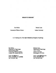
in the execution in a cyclic fashion, where first processor would start tracking counters from first counter group, second processor from second counter group, and so on. To enhance further this spacial distribution of counter groups, we also configured each processor to switch its active counter group to the next one every five seconds. The execution itself typically took several minutes. Since, in all our experiments, we used minimum 16 processors, we were able to assign each of the ten counter groups to at least one processor. An example of a distribution of counter sets is presented in Figure 1, where 8 CPUs are involved, with 4 counter sets, and the selected counter being in set #1. At any given moment two of the processors are tracking the selected counter. We calculated average value of each counter for every CPU burst throughout the whole execution time, that way producing a flattened trace as a unified timeline of all the collected counters. Finally, since the resulting time series consisted of millions of short periods, we implemented a simple bucketing algorithm that divided the whole execution time in 200 equal segments and averaged our target values over each of those segments. Figure 2 depicts the trace flattening process, by showing only those execution segments that track the selected counter. Each of the segments consists of a series of individual CPU bursts that contain the values of the selected
counter. Flattened trace is divided into segments that correspond to the CPU bursts. Counter value for each segment is then derived from the two CPU bursts as the sum of their selected counter values, and by taking into account respective burst duration. Importantly, our characterization methodology is validated against the performance reported by well-known benchmarks such as LINPACK [7], the de-facto benchmark of floating-point performance for high-performance scientific computing. We base our analysis on a set of four applications, selected according to Simpson et al.’s survey of highperformance applications used in supercomputing centers across Europe [16], and chosen to represent the dominant scientific domains in the supercomputing centers surveyed. More importantly, the analysis showed that each of the selected applications stress different aspects of the memory system. The selected applications include: • GADGET (GAlaxies with Dark matter and Gas intEracT). A code for cosmological simulations of structure formation. It computes gravitational forces with a hierarchical tree algorithm, optionally in combination with a particle-mesh scheme for long-range gravitational forces. It is one of the most often used applications, representing the area of astronomy and cosmology. From the four applications that we used, GADGET had the highest requirements of memory size. • MILC (MIMD Lattice Computation). A set of codes for doing simulations of four dimensional SU(3) lattice gauge theory, represents the area of particle physics, and in our analysis had the highest requirements of memory bandwidth. • WRF (Weather Research and Forecasting). A nextgeneration mesocale numerical weather prediction system designed to serve both operational forecasting and atmospheric research needs. It is a well-known DEISA benchmark from the area of earth and climate. In our analysis, it is characterized as the application that is bound by the system’s computational resources. • SOCORRO — self-consistent electronic-structure calculations utilizing the Kohn-Sham formulation of density-functional theory. Calculations are performed using a plane wave basis and either norm-conserving pseudopotentials or projector augmented wave functions. This application mostly stresses the memory bandwidth. Each of the applications was executed on 16, 32, 64 and 128 processors, with the exception of GADGET — whose memory footprint could not fit on 16 MareNostrum blades. The input sets in all of the analyzed applications remained unchanged while scaling the number of processors.
With the advance in multicore design, and scaling the number of processors, it is reasonable to expect that the input sets of the applications being executed will also grow. It is clear that the memory requirements of such applications can only be higher than the ones that we evaluate, and that the memory technology limits can be reached sooner than projected in this work.
4 Memory footprint In this section, we try to quantify the memory footprint of parallel applications, as a key factor determining the size requirements of both on-chip and off-chip memory in future CMPs. Table 1 shows the average and maximum per-processor footprints for the applications under analysis. The total footprint is calculated as the number of processors multiplied by the maximum per-processor footprint. In case that the memory system does not satisfy the maximum footprint requirements of a given application, it would crash when left out of memory space. The table also shows the relative reduction in maximum per-processor footprint, as well as relative increase in total footprint, both compared to the execution with half as many processors. Figures 3a to 3d describe the progression of the average per-processor memory footprint for the four applications. The vertical axis shows the memory footprint in GB, and the horizontal axis depicts the progression of normalized
Memory footprint (per core)[GB]
Memory footprint (per core)[GB]
1.8 1.6 1.4 1.2 1 0.8 0.6 0.4 0.2 0 0
20
40 60 80 Execution time[%]
0.7 0.6 16 processors 32 processors 64 processors 128 processors
0.5 0.4 0.3 0.2 0.1 0
100
0
(a) GADGET 0.2 0.18 0.16 0.14 0.12 0.1 0.08 0.06 0.04 0.02 0 0
20
40 60 80 Execution time[%]
(c) WRF
20
40 60 80 Execution time[%]
100
(b) MILC Memory footprint (per core)[GB]
32 GADGET 64 128 16 32 MILC 64 128 16 32 WRF 64 128 16 32 SOCORRO 64 128
Footprint [GB] Maximum Total per CPU footprint footprint total avg max reduction increase 1.27 1.80 57.69 0.75 0.98 62.58 45.76% 8.49% 0.49 0.68 86.85 30.61% 38.78% 0.57 0.61 9.71 0.29 0.31 9.90 49.00% 1.99% 0.15 0.16 10.28 48.10% 3.81% 0.07 0.09 11.04 46.29% 7.41% 0.19 0.20 3.17 0.12 0.12 3.90 38.39% 23.21% 0.07 0.07 4.77 38.85% 22.30% 0.05 0.05 6.78 28.94% 42.12% 0.18 0.20 3.19 0.11 0.12 3.96 37.82% 24.36% 0.08 0.09 5.56 29.87% 40.25% 0.06 0.07 8.68 21.93% 56.14%
Memory footprint (per core)[GB]
Application
#CPUs
Table 1. The per-processor and overall memory footprints measured for the benchmark applications.
100
0.2 0.18 0.16 0.14 0.12 0.1 0.08 0.06 0.04 0.02 0 0
20
40 60 80 Execution time[%]
100
(d) SOCORRO
Figure 3. Evolution of the memory footprint
execution time. As expected in a strong scalability case, when we divide the same working set across a large number of processors, the per-processor memory footprint decreases as the number of processors participating in the computation increases. However, doubling the number of processors does not halve the size of the per-processor memory footprint. For both WRF and SOCORRO, doubling the number of processors only reduces the per-processor memory footprint by 2040%. Scaling is somewhat better for GADGET, for which scaling from 32 to 64 processors reduces the per-processor footprint by 45%, while scaling further to 128 processors reduces the footprint by only 30% more. Scaling for MILC is very good, as footprint reduction is very close to 50%. This suboptimal reduction in per-processor memory footprint is partially an artefact of using distributed memory applications, and it is caused by the replication of data between processors. Many distributed algorithms that employ spatial metrics to partition the entire problem set into segments, replicate segment borders among processors assigned with neighbouring segments. For example, partitioning a large matrix into small sub-matrices will typically involve replication of the rows and columns on segment borders. Therefore, reducing the per-processor segment size will inevitably increase the portion of the segment that constitute as part of its border — that is replicated on the processor assigned with the neighbouring segment, and thus increase the percentage of application data that is replicated among the nodes. As a result, total memory footprint increases along with the number of processors, as shown in
256 GADGET MILC WRF SOCORRO
Table 2. The memory bandwidth measured at different levels of the memory system for the benchmark applications.
64 32
Application
16 8
2 8
16
32
64
128 256 512 Number of processors
1K
2K
4K
Figure 4. Projections of overall memory footprints for large-scale parallel systems, based on a linear regression model.
Table 1. Shared memory environment, on the other hand, would not experience an increase in the total memory footprint, but still, we would see more impact on the working set captured by caches and increase in cache coherency traffic. Figure 4 extends the measurements through linear regression, and projects the total memory footprint for larger number of processors. The vertical axis on Figure 4 shows the estimated total footprint, and the horizontal represents the number of processors. Points on the graph represent the actual values measured from the executed application, while the lines show the linear regression of the total footprint for the particular application (the projection lines do not have a linear appearance due to the logarithmic axes). The amount of data replication identified in the discussed benchmarks also supports our projections about the usefulness of caching: even though each processor participating in a parallel computation needs to access data originally assigned to its neighbour, aggressive caching can capture such data-sharing patterns and prevent the data from going off-chip, thereby saving precious memory bandwidth. More details about this are provided in Section 5.2. In summary, we see that future manycores consisting of more than 100 cores must be directly backed with a few dozens GBs of main memory in order to support scientific workloads.
5 Memory bandwidth 5.1
32 64 128 16 32 MILC 64 128 16 32 WRF 64 128 16 32 SOCORRO 64 128 GADGET
4
Bandwidth scales linearly
Consolidating multiple cores on a single chip imposes much higher bandwidth requirements on the shared components of the memory system — namely the off-chip memory and the shared caches. In order to predict those require-
#CPUs
Estimated total footprint [GB]
128
Average bandwidth Total per processor [GB/s] memory Memory L2 cache L1 cache bw. [GB/s] 0.114 4.50 11.04 3.57 0.100 3.66 10.96 6.26 0.068 2.90 10.91 8.44 0.815 0.52 14.12 12.73 0.598 0.80 13.47 18.70 0.604 0.75 13.38 37.78 0.617 0.77 13.29 77.18 0.117 1.55 7.35 1.82 0.102 1.87 8.32 3.18 0.091 1.70 8.87 5.69 0.050 1.95 10.09 6.22 0.331 4.14 15.35 5.18 0.279 3.35 13.39 8.72 0.212 2.83 12.08 13.23 0.228 2.73 11.75 28.49
ments, we measured the per-processor bandwidth consumed by each benchmark at three levels: the off-chip memory, L2 cache, and L1 cache. Table 2 shows the average per processor bandwidth in each of the three levels: the off-chip memory, L2 cache, and L1 cache. It also shows the estimated total memory bandwidth required by all the processors involved in the execution combined. Figure 5 uses linear regression to present the estimated total memory bandwidth required by each application for a particular processor count. Horizontal axis presents the number of processors used for the execution, while the vertical axis presents the memory bandwidth. Points in the figure show the actual measured values, while the lines show the linear regression, that is calculated in order to estimate the total bandwidth requirements for a larger number of processors. Each series stands for one of the four benchmark applications used in our evaluation. Both Figure 5 and Table 2 show that bandwidth requirements for MILC and SOCORRO grow almost linearly with the increase of the number of processors. MILC is the most demanding application in terms of bandwidth, and requires close to 80 GB/s when executed on 128 processors. SOCORRO behaves in a similar way, reaching almost 30 GB/s for 128 processor execution. GADGET and WRF do not have such a steady growth, and for different reasons. GADGET tends to benefit from an increased cache effectiveness, due to the reduced work-
128 GADGET MILC WRF SOCORRO
Estimated total bandwidth [GB/s]
64 32 16 8 4 2 1 8
16
32
64 128 256 Number of processors
512
1K
2K
Figure 5. Projections of overall memory bandwidth for large-scale parallel systems, based on linear regression.
0.2
Memory bandwidth (per core) [GB/s]
16 processors 128 processors
0.15
0.1
0.05
0 0
20
40 60 Execution time [%]
80
100
Figure 6. WRF memory bandwidth
ing set per processor (as discussed in Section 4), and, therefore, less bandwidth is required from the main memory. The L1 cache bandwidth stays on the same level, which suggests that the total bandwidth requirements of each processor barely changes with the increase of the number of processors. On the other hand, WRF experiences a different behaviour, as its initialization and finalization phase, which hardly produce any off-chip memory traffic, start to occupy a significant part of the total execution, with the increased number of processors. In contrast, its computation phase, which is very memory demanding, becomes relatively shorter and shorter. Therefore, the average bandwidth over the entire execution decreases, although it stays on the same level during the computation phase. Figure 6 demonstrates this phenomenon by showing how bandwidth progresses with time. Horizontal axis represents normalized execution time, and vertical axis off-chip memory band-
width. For brevity, Figure 6 depicts memory bandwidth for 16 and 128 processors only. In summary, we observe that future manycore systems consisting of more than 100 cores may easily require more than 100 GB/s of main memory bandwidth. Modern architectures such as Intel Nehalem-EX [10] or IBM Power7 [8] employ 4 and 8 DDR3 channels respectively, peaking at 102.4 GB/s of bandwidth. Knowing that the sustained bandwidth is typically 20%–25% lower due to page and bank conflicts, we conclude that such large-scale systems will need to provide higher bandwidth to support highperformance scientific computing.
5.2
Cache effectiveness
Compared with the off-chip bandwidth, the observed L2 cache bandwidth is typically an order of magnitude higher. This is understandable as the L2 cache hits filter bandwidth that would otherwise go off-chip. The same conclusion would apply for L1 versus L2 bandwidth. To better understand the effectiveness of the caches, as well as the effect of increased parallelism on caches, we have investigated the relation between L1 and L2 cache hit rates, and off-chip memory bandwidth. In Table 3, we present L1 and L2 hit rates, as well as the effect they have on off-chip memory bandwidth per processor (also shown in Table 2). We already mentioned, in Section 5.1, the effect of increased cache effectiveness for GADGET. It is interesting to observe, from Table 3, that L1 cache is the one that makes the difference, although its size of 32 KB compared to GADGET’s extremely large working set of more than 0.5 GB per processor, seems relatively small. This could mean that GADGET has very regular memory access patterns, which target relatively small memory blocks, so that L1 cache can capture most of the memory accesses, and have increase in effectiveness as the size of the blocks decrease with higher number of processors. MILC, on the other hand, is a bit less demanding when having memory footprint in mind, which makes the transition from 16 to 32 processors (and from 0.57 to 0.29 GB of memory footprint) very favourable for L2 cache. Reduction in per-processor working set, led to a better locality of access patterns, and that way better fitting in L2 cache. Huge increase in L2 cache hit rate, from 39.31% to 57.66%, made the impact on filtering a great deal of off-chip memory traffic. Furtheremore, MILC’s scalability results in an increase in the relative duration of the initialization phase, compared to the total execution time, as the number of processors increase (similar to WRF). Therefore, the stable average hitrates of the different caches actually hide the fact that the different phases exhibit very distinct cache behavior, with
GADGET
MILC
WRF
SOCORRO
32 64 128 16 32 64 128 16 32 64 128 16 32 64 128
L1 cache L2 cache Mem. bw. hit rate hit rate [MB/s] 93.67% 97.58% 114.26 94.41% 97.40% 100.09 95.09% 97.77% 67.53 97.13% 39.31% 814.56 97.00% 57.66% 598.41 96.43% 55.80% 604.44 96.74% 56.07% 617.40 93.39% 93.15% 116.67 93.71% 94.94% 101.90 94.43% 95.02% 91.04 94.99% 97.57% 49.74 97.21% 92.74% 331.31 97.38% 92.47% 279.16 96.83% 93.20% 211.63 97.02% 92.45% 227.91
the initialization phase enjoying an impressive L1 hit rate of over 99%, whereas the L1 hit-rate of computation phases decreases as the level of parallelism increases — from 97% for 32 processors, down to around 95% for 128 processors. These lower hit-rates in the computational phases, particularly when running on 128 processors, have a direct impact on the memory bandwidth (which increases from 598.41 to 617.40 MB/s) and memory related pipeline stalls. WRF has particularly high hit rate for both L1 and L2 cache, and therefore, only a small fraction of all memory accesses ends up reaching off chip memory. Even a seemingly minor increase in cache effectiveness from 93% to 97% can lead to a big decrease in off-chip memory traffic. If we combine this fact with the effect of relative reduction of WRF’s computation phase (discussed in Section 5.1, and shown in Figure 6), the resulting memory bandwidth per processor drops from 116.67 MB/s with 16 processors down to 49.74 MB/s with 128 processors. Effective caching has a direct impact on memory bandwidth, as shown on Figure 7. The figure shows the relation between off-chip memory bandwidth (shown on top subplot), and L2 cache hit rate (shown on bottom subplot), of a MILC executed on 32 processors. Due to the lack of space, we omit similar cache effectiveness figures for other applications. With a constant memory access rate and a constant L1 hit rate, the two depicted metrics are inversely proportional. The figure clearly identifies the initialization phase and two iterations, with L2 cache hit rate peaking to more than 80% during the end of each iteration. As the hit rate increases, the off-chip memory goes from 0.6–0.7 GB/s down
Memory bandwidth [GB/s]
Application #CPUs
L2 hit rate [%]
Table 3. Hit-rates measured for the different cache levels.
0.9 0.8 0.7 0.6 0.5 0.4 0.3 0.2 0.1 0 100 80 60 40 20 0 0
10
20
30
40 50 60 Execution time [%]
70
80
90
100
Figure 7. MILC 32p L2 cache effectiveness to ∼0.3 GB/s. In summary, caches prove to be effective bandwidth filters, and any further advances in their performance may delay reaching the point when bandwidth requirements of an application can no longer be supported by the existing memory technologies. However, contrary to the memory footprint, maximum bandwidth requirements imposed by the running application do not need to be met in order for the application to run. Of course, it is preferred that the memory system provides the required bandwidth, but if not, the application would not crash. It is clear that the insufficient bandwidth would hurt the performance of the system, but we can only speculate about this performance degradation. For example, if memory provides only 50% of the bandwidth that one execution segment requires, and if we assume that this segment is completely memory bound (there are no stall cycles due to any other core resource but the memory), it would be safe to say that this execution segment would run half of its maximum speed.
6 CPI stack The cycles per instruction (CPI) metric is defined as the average number of processor cycles needed to complete one instruction. For any execution segment, it is calculated as a total of elapsed cycles divided by the number of completed instructions. A low CPI value means that the system resources are better utilized, and the architecture operates closer to its peak performance. The PowerPC 970MP processor dispatches instructions to its back end in groups of five. Therefore, the theoretical execution throughput is five instructions per cycle, or conversely, 51 = 0.2 cycles per instruction. Several restrictions in PowerPC 970’s dispatch queue, as well as insufficient instruction-level parallelism in real applications, prevent CPI from being as low as 0.2. Instead, our experiments
Other completion stalls (9) Stall by FPU inst (8) Stall by FXU inst (7) Stall by LSU basic latency (6) Stall by D-cache miss (5) Stall by LSU reject (4) Other completion table empty cycles (3) I-cache miss penalty (2) Completion cycles (1)
Ind Clr
5
4
CPI
9
8
3
2
1
7
0 0
200
400
600 800 Execution time[s]
1000
1200
(a) MILC 16p
6 5
Other completion stalls (9) Stall by FPU inst (8) Stall by FXU inst (7) Stall by LSU basic latency (6) Stall by D-cache miss (5) Stall by LSU reject (4) Other completion table empty cycles (3) I-cache miss penalty (2) Completion cycles (1)
5
4
4
CPI
Total cycles
Table 4. CPI stack model CPI stack component others (Stall by BRU/CRU inst, flush penalty (except LSU flush)) Stall by FPU Stall by basic latency FPU inst Stall by any form of FDIV/FSQRT inst Stall by FXU Stall by basic latency Completion FXU inst Stall by any form of stall cycles DIV/MTSPR/MFSPR Stall by basic latency Stall by D-cache miss Other reject Stall by Stall by LSU inst Stall by translation reject (rejected by ERAT miss) others (Flush penalty etc.) Completion Branch redirection table empty (branch misprediction) penalty cycles I-cache miss penalty overhead of cracking/microcoding Completion and grouping restriction cycles PowerPC base completion cycles
3
3
2
2
1
1
0 0
100
200
300
400 500 Execution time[s]
600
700
800
(b) MILC 32p
show the CPI in real applications gets usually between 1 and 1.5, sometimes even as high as 3 (5–15x slower than the peak throughput). The CPI stack model, which is the breakdown of CPI value to the individual latencies contributed by different micro-architectural resources, can therefore be used to determine the key factors that impede performance. Each component in the stack describes the average number of cycles an instruction stalled on a particular core resource (like Load/Store unit, or Floating Point unit). We construct the CPI stack using the PowerPC 970MP performance counters [13]. Some of them are specific to PowerPC 970MP architecture, so the CPI stack model for other architectures may contain minor differences. The individual stack components are described in Table 4. The table also includes both index and color used in the CPI stack figures presented in this section. Figures 8–11 present the evolution of the CPI stack throughout the entire run of the benchmark applications (due to space constraints, we only show the full evolution of a subset of the applications and architectural configurations). The global averages are shown in Figure 12. For example, MILC running on 16 processors (Figure 8a) requires 3.2 cycles to complete an instruction, of which an average
Figure 8. MILC CPI stack
0.2 cycles are spent on committing the instruction, 2.3 cycles on stalls associated with the load/store unit (LSU), 0.5 cycles on the fixed-point and floating-point units (FXU and FPU, respectively), and 0.2 cycles on other stalls. All the presented CPI stack figures show that both Icache miss penalty and branch misprediction penalty have negligible impact on performance. This means that the Icache is large enough for all the tested applications, so that it rarely experiences a miss. Also, the branch prediction shows efficiency, as expected for scientific applications [6]. Importantly, these findings are not affected by the increase in parallelism. Figure 8 shows that scaling MILC from 16 to 32 processors dramatically decrease all LSU related stalls, from 2.3 cycles for 16 processors, to 1.5 cycles for 32 processors. The benefit is evident both in the overall CPI value, as well as the execution time. As shown in Section 5.2, this performance improvement is due to MILC’s reduction in per-processor memory footprint. When running on 16 processors, MILC’s working set exceeds the size of data cache. But the increase in the number of processors reduces the
2.5
2.5 Other completion stalls (9) Stall by FPU inst (8) Stall by FXU inst (7) Stall by LSU basic latency (6) Stall by D-cache miss (5) Stall by LSU reject (4) Other completion table empty cycles (3) I-cache miss penalty (2) Completion cycles (1)
2
2
CPI
1.5
CPI
1.5
Other completion stalls (9) Stall by FPU inst (8) Stall by FXU inst (7) Stall by LSU basic latency (6) Stall by D-cache miss (5) Stall by LSU reject (4) Other completion table empty cycles (3) I-cache miss penalty (2) Completion cycles (1)
1
1
0.5
0.5
0
0 0
100
200 300 Execution time[s]
400
500
0
100
(a) WRF 32p
200
300 400 Execution time[s]
500
600
(a) GADGET 32p CPI stack
2.5
0.7 L1 loads per instruction L1 stores per instruction
Other completion stalls (9) Stall by FPU inst (8) Stall by FXU inst (7) Stall by LSU basic latency (6) Stall by D-cache miss (5) Stall by LSU reject (4) Other completion table empty cycles (3) I-cache miss penalty (2) Completion cycles (1)
2
0.5 0.4
CPI
1.5
0.6
0.3
1
0.2 0.5 0.1 0
0 0
50
100
150 200 Execution time[s]
250
300
0
100
200
300 400 Execution time[s]
500
600
(b) WRF 128p
(b) GADGET 32p L1 cache traffic
Figure 9. WRF CPI stack
Figure 10. GADGET CPI stack and L1 cache traffic
per-processor memory footprint such that it fits in the cache for the 32 processor configuration. With further increase in number of processors, we do not see such a dramatic improvement in CPI value, because the working set already fits in cache. In the case of WRF, the evolution of the CPI stack clearly reveals the application’s initialization, computation and finalization phases (same as those observed in Section 5.1), which are clearly distinguished by their FPU usage. The initialization and finalization phases hardly exhibit any FPU stalls. In contrast, the computation phase is highly FPU dependent as about half of its instructions’ stall time is associated with the FPU. As the number of processors increases, WRF’s scalability allows its computation phase to shorten. However, the initialization and finalization phases are evidently non-scalable and do not benefit from the increased parallelism. As such, their execution time does not change, and, therefore, begin to dominate the overall execution time. This implies that the application’s overall scalability is limited, unless the input set size increases. GADGET’s most obvious CPI stack patterns, shown in
Figure 10a, are significant fluctuations of the overall CPI value, revealing three periodic iterations. Parts of each iteration with low FPU usage have an overall high CPI value, whereas parts with high FPU usage have low CPI value. When correlating this with the frequency of memory accesses, presented in Figure 10b, it is noticeable that high CPI value corresponds to high memory traffic (more specifically high number of stores). This also justifies fairly large number of LSU stalls (LSU reject, D-cache miss and LSU basic latency) in this part of the iteration. Therefore, each of the three iterations can be divided into a communication phase (low FPU usage, lots of memory accesses, high bandwidth, high CPI), and a computation phase (high FPU usage, few memory accesses, low bandwidth, low CPI). We do not see much variation in GADGET graphs for 32, 64 or 128 processors. Finally, SOCORRO is yet another example of an application that is memory bound, as we can observe in Figure 11. Even though its per-processor working set easily fits in the cache (Section 5.2), its periodic LSU and cache stalls imply
2
4 Other completion stalls (9) Stall by FPU inst (8) Stall by FXU inst (7) Stall by LSU basic latency (6) Stall by D-cache miss (5) Stall by LSU reject (4) Other completion table empty cycles (3) I-cache miss penalty (2) Completion cycles (1)
3 CPI stack
CPI
1.5
Other compleion stalls (9) Stall by FPU inst (8) Stall by FXU inst (7) Stall by LSU basic latency (6) Stall by D-cache miss (5) Stall by LSU reject (4) Other completion table empty cycles (3) I-cache miss penalty (2) Completion cycles (1)
3.5
1
2.5 2 1.5 1 0.5
0.5
0
150 200 Execution time[s]
250
300
28p O1 RR 4p CO O6 SO RR 2p CO O3 SO RR 6p CO O1 SO RR CO
100
SO
50
28p F1 WR 4p F6 WR 2p F3 WR 6p F1 WR
0
p 128 LC MI 64p LC MI 32p LC MI 16p LC MI p 128 ET DG p GA ET 64 DG p GA ET 32 DG
GA
0
Figure 11. SOCORRO 128p CPI stack
Figure 12. CPI stack average values
that each of its iterations operates on a separate chunk of data. This data is transferred from the memory to the cache, processed, and stored back to memory. This scanning access pattern puts a significant load on the memory system, regardless of the cache size or number of processors. Figure 12 presents the average CPI stack for all the applications tested. First, it appears that GADGET’s computation pattern does not change when increasing the number of processors to 128, as indicated by its similar CPI stacks. For MILC, we observe a gradual increase in CPI (following the aforementioned drop when increasing the number of processors from 16 to 32), which is mostly attributed due to LSU related stalls. This is a consequence of a decrease in L1 cache effectiveness, and therefore, higher memory traffic (discussed in Section 5.2). WRF, on the other hand, enjoys a slight decreasing CPI trend, due to an increase in the relative duration of memory intensive phases, and a decrease of computationally intensive phase. Therefore, all LSU related stall values grow, while FPU related stall values decline. Finally, SOCORRO’s CPI seems to benefit slightly with scaling number of processors, mostly due to a lower amount of LSU related stalls. In summary, LSU related stalls seem to be the most dominant CPI stack component in the applications tested. The exceptions are GADGET and WRF, whose computation phases are limited by FPU stalls. It indicates that memory hierarchy could have an exceptionally high impact on performance of the future manycores. It is also clear that wider superscalar approach can have a limited impact, and the only ones that could see the benefit are FPU intensive applications. CPI stack components not related to LSU can give us an indication on how scaling compute performance relates to scaling bandwidth requirements. That is, by shortening the time to process a block of data, we would increase the processing throughput, and, unless the cache hierarchy gets changed, increase the off-chip memory bandwidth demand.
Therefore, making the same application analysis we have done in this work on a platform that outperforms PowerPC 970, would make the slope of our bandwidth projections on Figure 5 steeper, and reach memory bandwidth limits with fewer number of processors.
7 Arithmetic performance In previous section we presented the impact of memory system on overall architectural performance, expressed as a rate of executed instructions. This section brings more focus on arithmetic performance, expressed as a rate of floating point operations (FLOPS) executed — probably the most important metric for determining supercomputer performance. For PowerPC 970MP architecture, the total number of floating point operations in an execution segment is calculated as a sum of the number of operations in each floating point unit, and the number of fused multiply-adds. Each floating point unit can process one floating point and one fused multiply-add instruction in a single cycle. Since we have two floating point units per core, maximum number of floating point operations per cycle is 4, which would give a theoretical maximum of 9.2 GFLOPS on a machine running at 2.3 GHz. All our calculations related to the arithmetic performance of a system, excluded execution segments that did not contain any floating point operations. This is done to estimate better efficiency of floating point units during computation phases, eliminate changes in relative duration of computation phases compared to initialization and finalization phases, and enable correlation of memory and arithmetic performance through bandwidth-to-performance ratio. Section 6 gives an indication on the execution segments that utilize the available floating point resources. Figure 13 presents average and maximum floating-point performance of our applications under study. The figure
Arithmetic performance [GFLOPS]
10 Maximum Average 8
6
4
2
0
p
16p CK PA LIN 28p O1 RR 4p 6 CO SO RRO p 32 CO SO RRO p 16 CO SO RRO CO
SO
28 F1 WR 64p F WR 32p F WR 16p F WR
p 128 LC MI 64p LC MI 32p LC MI 16p LC MI p 128 ET p DG 4 GA ET 6 DG 2p GA ET 3 DG
GA
Figure 13. Arithmetic performance
Bandwidth-performance ratio [B/flop]
3 2.5 2 1.5 1
Figure 14 shows bandwidth-performance ratios for all the applications under study, averaged over their time spent in computation phases. As we can see, most of the applications, with the exception of MILC, fit very well with projected bandwidth-performance ratio of 0.5 B/flop, that has been mentioned before. However, previous measurements of average arithmetic performance made clear that the reason for this ratio being relatively high is not high bandwidth requirements, but low arithmetic performance achieved. And indeed, in case of MILC, which performs only 0.3– 0.4 GFLOPS bandwidth-performance ratio gets considerably higher than the other applications. On the other hand, LINPACK, with its average 5.2 GFLOPS, brings down the ratio to only 0.08 B/flop. In conclusion, we observe that dimensioning memory bandwidth based on peak arithmetic performance may be inadequate, due to the overwhelming underutilization of processor arithmetic performance in real applications. In this case, estimates of 4.6 GB/s of memory bandwidth per processor are considerably above the effective requirements. This is confirmed by the results presented in Section 5, which shows that none of the test applications exceeds bandwidth of 1 GB/s.
0.5
8 Conclusions
0
16p CK PA LIN 28p O1 RR 64p CO SO RRO p 32 CO SO RRO p 16 CO SO RRO CO SO
28p F1 WR 64p F WR 32p F WR 16p F WR
p 128 LC MI 64p LC MI 32p LC MI 16p LC MI p 128 ET p DG 4 GA ET 6 DG 2p GA ET 3 DG GA
Figure 14. Bandwidth-performance ratio
shows that real applications achieve only a small fraction of the peak performance. This sub-optimal utilization of all the floating point resources that the architecture provides can be attributed to various data dependencies the inhibit ILP. This is consistent with the results for the highly optimized LINPACK benchmark, which only achieves an average 5.2 GFLOPS — only 57% of the peak 9.2 GFLOPS processor performance. System designers often use processor’s arithmetic performance measurements to dimension the required performance of other computer system components. Dimensioning memory bandwidth is often based on a ratio of maximum bandwidth and maximum theoretical rate of floating point operations. A common rule of thumb for obtaining optimal performance is to keep this ratio around 0.5 bytes per flop. This means that a processor capable of achieving 9.2 GFLOPS should rely on memory that supplies 4.6 GB/s of bandwidth. However, our analysis show that this ratio is heavily overestimated, and that it should not be taken into account at all, mostly due to the underutilization of floating point resources in real applications.
The increasing multicore density is putting a proportionally higher stress on the memory system. It is unclear if current memory system architectures will be able to sustain the increasing number of on-chip cores. In this paper we evaluate the memory system requirements of HPC applications, running on the MareNostrum supercomputer at BSC, and characterize the memory performance requirements of future manycore designs. We show that memory size requirements are actually closer to 0.5 GB per core, and memory bandwidth requirements are under 0.1 Bytes per peak flop. This is in contrast to the existing (undocumented) rule of thumb for designing the memory system of a supercomputer that call for 2GB of memory per core, and 0.5 bytes/flop peak bandwidth. Next, we show that on-chip caches, originally placed to mitigate memory latencies, are very effective at filtering bandwidth to the off-chip memory, with on-chip bandwidth requirements being orders of magnitude higher. Moreover, we evaluate the actual flops achieved by the applications, and show them to be only a fraction of the peak performance. It is only when computing bytes per real flops that the bandwidth requirements get close to the 0.5 mark, but it is due to the low flops, not to the high bandwidth. In light of our findings, we expect that current memory architectures based on on-chip memory controllers and multiple parallel DDR channels should be able to sustain multicores for the next decade.
Acknowledgements This research is supported by the Consolider contract number TIN2007-60625 from the Ministry of Science and Innovation of Spain and the TERAFLUX project (ICT-FP7249013). Y. Etsion is supported by a Juan de la Cierva Fellowship from Ministry of Science and Innovation of Spain.
References [1] G. Abandah and E. Davidson. Configuration independent analysis for characterizing shared-memory applications. In Intl. Parallel Processing Symp., pages 485–491, Mar 1998. [2] A. Agarwal, L. Bao, J. Brown, B. Edwards, M. Mattina, C.C. Miao, C. Ramey, and D. Wentzlaff. Tile processor: Embedded multicore for networking and multimedia. In Hot Chips, Aug 2007. [3] S. R. Alam, R. F. Barrett, J. A. Kuehn, P. C. Roth, and J. S. Vetter. Characterization of scientific workloads on systems with multi-core processors. In IEEE Intl. Symp. on Workload Characterization, pages 225–236, Oct 2006. [4] M. Bhadauria, V. M. Weaver, and S. A. McKee. Understanding parsec performance on contemporary cmps. In IEEE Intl. Symp. on Workload Characterization, Oct 2009. [5] D. Burger, J. R. Goodman, and A. K¨agi. Memory bandwidth limitations of future microprocessors. In Intl. Symp. on Computer Architecture, pages 78–89, 1996. [6] Z. Cvetanovic and R. E. Kessler. Performance analysis of the alpha 21264-based compaq es40 system. In Intl. Symp. on Computer Architecture, pages 192–202, 2000. [7] J. Dongarra, J. Bunch, C. Moler, and G. Stewart. Linpack. www.netlib.org/linpack. [8] R. Kalla, B. Sinharoy, W. J. Starke, and M. Floyd. Power7: IBM’s next-generation server processor. IEEE Micro, 30:7– 15, 2010. [9] P. Kongetira, K. Aingaran, and K. Olukotun. Niagara: A 32way multithreaded Sparc processor. IEEE Micro, 25:21–29, 2005. [10] S. Kottapalli and J. Baxter. Nehalem-EX CPU architecture. In Hot Chips, Aug 2009. [11] L. Liu, Z. Li, and A. H. Sameh. Analyzing memory access intensity in parallel programs on multicore. In Supercomputing, pages 359–367, 2008. [12] The MareNostrum system architecture. http://www.bsc.es/plantillaA.php?cat id=200. [13] A. Mericas. Performance monitoring on the POWER5TM microprocessor. In Performance Evaluation and Benchmarking, pages 247–266. CRC Press, 2005. [14] R. C. Murphy and P. M. Kogge. On the memory access patterns of supercomputer applications: Benchmark selection and its implications. IEEE Trans. Computers, 2007. [15] L. Seiler, D. Carmean, E. Sprangle, T. Forsyth, P. Dubey, S. Junkins, A. Lake, R. Cavin, R. Espasa, E. Grochowski, T. Juan, M. Abrash, J. Sugerman, and P. Hanrahan. Larrabee: A many-core x86 architecture for visual computing. IEEE Micro, 29(1):10–21, 2009.
[16] A. D. Simpson, M. Bull, and J. Hill. Identification and Categorisation of Applications and Initial Benchmarks Suite, 2008. www.prace-project.eu. [17] S. C. Woo, M. Ohara, E. Torrie, J. P. Singh, and A. Gupta. The SPLASH-2 programs: characterization and methodological considerations. In Intl. Symp. on Computer Architecture, pages 24–36, 1995.