the hybrid principle of maximum and the method of dynamic programming for the systems of this class ... The problem of optimal control in the hybrid systems is especially ... is the set of permissible values of the control inputs (set of controls);.
c Pleiades Publishing, Ltd., 2009. ISSN 0005-1179, Automation and Remote Control, 2009, Vol. 70, No. 5, pp. 787–799. � c V.V. Azmyakov, R. Galvan-Guerra, A.E. Polyakov, 2009, published in Avtomatika i Telemekhanika, 2009, No. 5, pp. 51–64. Original Russian Text �
DETERMINATE SYSTEMS
On the Method of Dynamic Programming for Linear-Quadratic Problems of Optimal Control in Hybrid Systems V. V. Azmyakov,∗ R. Galvan-Guerra,∗ and A. E. Polyakov∗∗ ∗
Research and Advanced Studies Center, National Polytechnical Institute, Mexico, United Mexican States ∗∗ Voronezh State University, Voronezh, Russia Received May 21, 2008
Abstract—For a sufficiently wide class of the linear hybrid systems, an algorithm of optimal feedback control was proposed. Consideration was given to the hybrid control systems with autonomous switching, as well as the corresponding problems of the hybrid linear-quadratic optimal control based on the recently suggested principle of maximum. Interrelations between the hybrid principle of maximum and the method of dynamic programming for the systems of this class were discussed. The classical formalism was extended, the corresponding Riccati equations were obtained, and discontinuity of the “hybrid” Riccati matrix was proved. The computational aspects of the established theoretical results were considered. PACS number: 02.30.Yy DOI: 10.1134/S0005117909050075
1. INTRODUCTION Various types of hybrid and switched systems are used in the modern engineering to model complex control system in chemical, bioengineering, and aero-space industries, as well in the systems of industrial electronics [1–6]. Additionally, the hybrid models are encountered in the multiagent distributed control systems and systems for management of social processes ([4] for example). The control theory for a sufficiently long time considered the discrete-continuous dynamic systems and the switched systems. New outlooks for the studies of some important applications of the variable-structure technical systems were opened by the developing theory of the hybrid systems and corresponding numerical algorithms. The problem of optimal control in the hybrid systems is especially complicated because in the general case one faces not only the infinite-dimensional problem of optimization, but also the need for combinatorial enumeration due to the discrete part of the system. In this connection, the majority of the schemes of practical optimization were proposed for particular classes of the hybrid systems. Many of them were based on the recently established optimality conditions, see, for example, [6, 8–20], the rest being related more with the classical approaches to dynamic system optimization [1–3, 21, 22]. Recently, an interest to the first-order optimization methods and the corresponding computational schemes based on the gradient methods and the principle of maximum [8–11] was displayed. This is due primarily to the simplicity of their realization, reliability, and availability of the results enabling one to support their accuracy and convergence. At the same time, the dynamic programming-based approaches are inadequate to the hybrid linear systems and corresponding linear-quadratic problems of optimal control. Along with the numerical procedures based on the Pontryagin principle of maximum, for the classical problems of optimal feedback control, the main means of constructing the optimal trajectory are represented by the famous Bellman method of dynamic programming. The traditional 787
788
AZMYAKOV et al.
dynamic programming-based approach is also known to be equivalent to the method based on the Pontryagin principle of maximum (see, for example, [23,24]). The present study aims at examining the relation between these two approaches for the hybrid systems and determining the corresponding formalism of the Riccati equations. We note that the traditional theory of linear systems cannot be formally transferred to the hybrid case (see [22] for more detail). Therefore, it is necessary, to expand the theory at least for some particular classes of the hybrid systems. 2. OPTIMIZATION OF THE LINEAR HYBRID SYSTEMS We first describe in general terms the hybrid systems with autonomous switching [9–11,14,15,19] that are used in what follows. Definition 1. The linear hybrid system is an assembly of seven finite sets of elements {Q, X , {Uq }q∈Q , A, B, U, S}, where • Q is the finite set of discrete states (locations); • X = {Xq }q∈Q is the family of the state spaces Xq ⊆ Rn ; • {Uq }q∈Q , Uq ⊆ Rm is the set of permissible values of the control inputs (set of controls); • A = {Aq (·)}, B = {Bq (·)}, q ∈ Q is the family of continuously differentiable matrix functions Aq : R → Rn×n ,
Bq : R → Rn×m
characterizing system dynamics at the corresponding locations; • U is the class of permissible control functions; • S is a subset of the set of switching pairs Ξ, where Ξ := {(q, x, q � , x� ) : q, q � ∈ Q, x ∈ Xq , x� ∈ Xq� }. We consider a hybrid linear system satisfying Definition 1 over the time interval [0, tf ]. The reader is referred to [17–20] for more detailed description of various types of the hybrid and switched systems. Let U ∈ Rm be a convex and closed set. We assume that U := {u(·) ∈ L∞ m (0, tf ) : u(t) ∈ U
almost everywhere on
[0, tf ]} ,
where L∞ m (0, tf ) is the ordinary Lebesgue space of the measurable and bounded almost everywhere functions. We assume below that the set S of Definition 1 is characterized by the assembly of the switching hyperplanes Mq,q� := {x ∈ Rn : mq,q� (x) = 0}, where mq,q� : Rn → R, q, q � ∈ Q and mq,q� (x) = bTq,q� x + cq,q� are linear functions and bq,q� ∈ Rn and cq,q� ∈ R for each q, q � ∈ Q. These hyperplanes Mq,q� contain linear sets of the switching points where transition (switching) from the location q to the location q � may occur (see Fig. 1). We recall
M1, 2
M1, 3 M1, 4 Fig. 1. Example of space decomposition by the switching lines for the first location. AUTOMATION AND REMOTE CONTROL
Vol. 70
No. 5
2009
ON THE METHOD OF DYNAMIC PROGRAMMING
789
x fq1(x, u) fq2(x, u) θq 1 x1(·)
fq4(x, u) fq3(x, u)
x2(·) θq 2
t1
x3(·)
fq5(x, u)
x4(·) θq4
θq3
t2
t3
x5(·)
t4
tf
t
Fig. 2. Dynamics of the hybrid system.
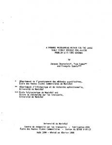
that in the general case by the location is meant the additional discrete characteristic of the system to which its own continuous state space Xq corresponds, rather than the domain of the continuous system state space as it is usually assumed in the variable-structure systems. We assume for simplicity that the introduced hyperplanes decompose the entire state space into the disjoint domains Xq . Obviously, in this case the projection of the set S on the product of the closures of the disjoint domains X¯q × X¯q� defines those points on the hyperplane Mq,q� where the transition between the locations q and q � may take place. It is assumed that this transition occurs at some isolated time instant called the time of switching tswitch ∈ [0, tf ]. We consider the hybrid linear systems with a fixed number of switchings at the time instants {ti }, i = 1, . . . , r − 1, r ∈ N, where 0 = t 0 < t 1 < . . . < tr = t f . We note that the sequence of the times of switching {ti } is unknown a priori. Since the hybrid system is at the location qi ∈ Q for all time instants t ∈ [ti−1 , ti ], i = 1, . . . , r, it is possible to introduce the notion of the hybrid trajectory of the system at hand (see, for example, [10]). Definition 2. The permissible hybrid trajectory of the system considered in Definition 1 is the assembly of three interrelated elements X = (x(·), {qi }i=1,...,r , τ ), where x(·) is the continuous system trajectory, {qi }i=1,...,r is the finite sequence of the realized locations (discrete trajectory), and τ = (t1 , . . . , tr )T is the corresponding sequence of the switching times such that for x(0) = � / Mq,q� , each i = 1, . . . , r, and any permissible control u(·) ∈ U. And we have that x0 ∈ q,q � ∈Q
•
•
xi (·) = x(·)|(ti−1 ,ti ) ∈ Xqi = Rn is the absolute continuous function over the interval (ti−1 , ti ) and continual over [ti−1 , ti ], i = 1, . . . , r; x˙ i (t) = Aqi (t)xi (t) + Bqi (t)ui (t) almost for all time instants t ∈ [ti−1 , ti ], where ui (·) is the contraction of the selected control function u(·) ∈ U to the interval [ti−1 , ti ].
The hybrid linear system satisfying Definitions 1 and 2 and the above assumptions will be denoted by LHS. Figure 2 depicts a qualitative picture of the hybrid system dynamics. We note that the pair (q, x(t)) is a hybrid state vector at the time instant t, where q defines the location q ∈ Q and x(t) ∈ Xq describes dynamics of the hybrid control system LHS. Since x(t) from Definition 2 is a continuous function, this concept describes the class of hybrid systems with continuous trajectories (without jumps). At the points of switching from the set Mq,q� , we have x(ti − 0) = x(ti + 0), i = 1, . . . , r. AUTOMATION AND REMOTE CONTROL
Vol. 70
No. 5
2009
790
AZMYAKOV et al.
Remark 1. The present paper considers hybrid systems such that in them “sliding” (see [25,26]) on one of the hyperplanes Mq,q� is ruled out. Theoretically speaking, in the hybrid system under consideration a sliding mode may occur on the plane Mq,q� only if Mq,q� = Mq� ,q . Therefore, in the case of coinciding hyperplanes, it is necessary to impose an additional geometrical condition on the system trajectories based on the well-known additional definition of Filippov [27]: bTqi ,qi+1 (λx˙ i (ti − 0) + (1 − λ)x˙ i+1 (ti + 0)) �= 0,
for
∀λ ∈ (0, 1),
� � � ∈ Q are two successive locations such that Mqi ,qi+1 = Mqi+1 where qi , qi+1 ,qi .
In virtue of Remark 1, the system dynamics prior and after the switching instant ti obeys different assemblies of system matrices {Ai , Bi } and {Ai+1 , Bi+1 }. Within the framework of the above definitions, for each permissible control u(·) ∈ U and each interval [ti−1 , ti ] (for each location qi ∈ R) there exists a single absolutely continuous solution of the linear differential equations from Definition 2, which implies that for each u(·) ∈ U there exists a unique almost everywhere absolutely continuous trajectory of system LHS. Additionally, the instants of switching {ti } and discrete trajectories {qi } of the system LHS are also defined uniquely. We note that the general evolutionary equation for the trajectory x(·) of the hybrid linear system LHS is representable as x(t) ˙ =
r � i=1
�
�
β[ti−1 ,ti ) (t) Aqi (t)xi (t) + Bqi (t)ui (t)
almost everywhere on
[0, tf ],
x(0) = x0 ,
(1)
where β[ti−1 ,ti ) (·) is the characteristic function of the interval [ti−1 , ti ), �
β[ti−1 ,ti ) (t) =
1, 0,
if t ∈ [ti−1 , ti ) otherwise
for i = 1, . . . , r. Let Sf ∈ Rn×n , Sq : R → Rn×n and Rq : R → Rm×m , where q ∈ Q. We assume that Sf is a symmetrical positive definite matrix, Sq (t) is the symmetrical positive semidefinite matrix for any time instant t ∈ [0, tf ] and any q ∈ Q, and Rq (t) is the symmetrical positive definite matrix for any t ∈ [0, tf ] and any q ∈ Q. Also, we assume that the matrix functions Sq (·), Rq (·) are continuously differentiable. We consider the following problem of linear quadratic optimization for the given system LHS: minimize J(u(·), x(·), τ ) on all permissible trajectories X of system LHS, r 1� 1 where J(u(·), x(·), τ ) := xT (tf )Sf x(tf ) + 2 2 i=1
�ti
(2)
xT (t)Sqi (t)x(t) + uT (t)Rqi (t)u(t)dt.
ti−1
Obviously, (2) is the problem of minimization of the quadratic objective Boltz functional J on the set of all possible trajectories of the given hybrid linear system. We note that here consideration is given to the problem of optimal hybrid control for system (1) without any constraint on its finite or intermediate states and the problem of hybrid optimization (2) has an optimal solution (uopt (·), Xopt (·)), where uopt (·) ∈ U and Xopt (·) belongs to the set of permissible trajectories from Definition 2. Existence of the optimal pair (uopt (·), Xopt (·)) for the above optimization problem follows from the general theory of existence of for the quadratic linear problems of optimal control with convex and closed set of permissible values U (see, for example, [24]). We apply to this problem the hybrid principle of maximum [10] and formulate for it the corresponding necessary optimality conditions. The general conditions for optimality of various hybrid dynamic systems can be found also in [10, 15, 18–20]. AUTOMATION AND REMOTE CONTROL
Vol. 70
No. 5
2009
ON THE METHOD OF DYNAMIC PROGRAMMING
791
Theorem 1. Let (uopt (·), Xopt (·)) be the optimal solution of the regular optimal control probopt lem (2). Then, there exist absolutely continuous functions ψi (·) defined on (topt i−1 , ti ), i = 1, . . . , r, and a nonzero vector of the Lagrange multipliers a = (a1 , . . . , ar−1 )T ∈ Rr−1 such that opt [topt i−1 , ti ],
(3)
= ψi+1 (topt i ) + ai bqi ,qi+1 ,
(4)
ψ˙ i (t) = −ATqi (t)ψi (t) + Sqi (t)xopt (t) almost everywhere on ψr (tf ) = −Sf xopt (tf ), �
opt ψi (topt i ) = ψi+1 (ti ) + ai
dmqi ,qi+1 xopt (topt i ) dx
where i = 1, . . . , r − 1. It is also known that for each permissible control u(·) ∈ U the corresponding Hamiltonian
�
Hqi (t, x, u, ψ) := ψi , Aqi (t)x + Bqi (t)u −
� 1� T x Sqi (t)x + uT Rqi (t)u 2
satisfies the following maximality conditions: �
�
max Hqi t, xopt (t), u, ψ(t) = Hqi t, xopt (t), uopt (t), ψ(t) , u∈U
where i = 1, . . . , r and ψ(t) :=
r
i=1
opt t ∈ topt , i−1 , ti
(5)
β[topt ,topt ) (t)ψi (t) for any t ∈ [0, tf ]. i−1 i
Remark 2. It deserves noting that Theorem 1 was proved for the conditions of no sliding modes over the switching surface Mq,q� . Of interest is a possible generalization of the necessary optimality conditions (hybrid principle of maximum) to the general hybrid systems and variable-structure systems admitting sliding over some switching surfaces (see Remark 1). We note that the conjugate variable ψ(·) is an absolutely continuous function over all open opt opt ∈ τ opt intervals (topt i−1 , ti ) for i = 1, . . . , r, but is discontinuous at the instants of switching ti of the hybrid system. At the same time, one can easily establish continuousness of the “full” Hamiltonian as the time function � opt (t) := H
r � i=1
�
β[topt ,topt ) (t)Hqi t, xopt (t), uopt (t), ψ(t) i−1 i
calculated for the optimal pair (uopt (·), Xopt (·)) and the corresponding conjugate variable ψ(·). � opt (·) is a function continuous over [0, tf ]. Theorem 2. Under the conditions of Theorem 1, H opt Proof. Let us consider the time interval [topt i−1 , ti ] and the corresponding Hamiltonian Hqi (t, x, u, ψ). � opt (t) is continuous over the open time interval (topt , topt ), i = 1, . . . , r. Obviously, the function H i−1 i Additionally, for the optimal pair (uopt (·), Xopt (·)) we obtain (see [19, 23])
�
∂J(uopt (·), xopt (·), τ opt ) . ∂topt i
No. 5
2009
opt opt opt (ti ), uopt (topt Hqi topt i ,x i ), ψ(ti ) = −
AUTOMATION AND REMOTE CONTROL
Vol. 70
792
AZMYAKOV et al.
Using (3) and (4) and the well-known representation for the variation of the objective function J (see, for example, [19, 23]), we obtain �
� opt (topt ) := Hq topt , xopt (topt ), uopt (topt ), ψ(topt ) H qi i i i i i i �
= Hqi+1 � opt
opt opt opt topt (ti ), uopt (topt i ,x i ), ψ(ti ) opt �
opt opt = Hqi+1 ti , xopt (topt (ti ), ψ(ti ) + ai i ), u
�
�
∂mqi ,qi+1 (xopt ) �� + ai � � opt ∂t t=t ∂(bqi ,qi+1
�i + cqi ,qi+1 ) �� � � ∂t
xopt
opt opt opt � opt opt = Hqi+1 topt (ti ), uopt (topt i ,x i ), ψ(ti ) =: Hqi+1 (ti ),
t=topt i
i = 1, . . . , r − 1.
(6)
� opt (t) not It is clear that the resulting relation (6) entails continuity of the introduced function H opt opt ∈ τ opt , only over the intervals (ti−1 , ti ), i = 1, . . . , r, but also at the instants of switchings topt i opt opt is the optimal sequence of the switching times on the trajectory X . where τ For a more general class of the hybrid systems with autonomous and controllable switchings, a similar result was established in [19, Theorem 2.2, p. 1590]. A special case of Theorem 2 is valid also for the hybrid system considered in [10]. The corresponding proofs of continuity of the optimal Hamiltonian as a time function are based on a generalization of the classical needle-shaped variations and their related formula for variations of the objective function in the considered hybrid problems of optimal control [13].
3. EXTENSION OF THE FORMALISM OF RICCATI EQUATIONS TO THE CASE OF LINEARLY QUADRATIC PROBLEMS OF OPTIMAL CONTROL The present section proposes to extend the classical method of dynamic programming to the hybrid linear quadratic problems of optimal control like (2). Let us consider the linear system (1), (3) for U ≡ Rm . The maximization condition (5) from Theorem 1 entails −1 T uopt i (t) = Rqi (t)Bqi (t)ψi (t),
opt t ∈ [topt i−1 , ti ).
This representation of the optimal control and simple facts from the theory of linear differential equations enable one to calculate (similar to [23, 24]) the optimal control uopt (·) for (2) as the optimal piecewise linear feedback defined over the set of all locations uopt (t) = uopt (xopt (t)) = −
r � i=1
β[ti−1 ,ti ) (t)Ci (t)xopt i (t),
(7)
(t)BqTi (t)Pi (t) is the matrix of feedback coefficients and Pi (·) is the Riccati matrix where Ci (t) := Rq−1 i related to the location qiopt ∈ Q. As in the classical case, we obtain for each location qiopt ∈ Q and opt almost all t from the open interval (topt i−1 , ti ) the differential equation (t)BqTi (t)Pi (t) + Sqi (t) = 0 P˙ i (t) + Pi (t)Aqi (t) + ATqi (t)Pi (t) − Pi (t)Bqi (t)Rq−1 i
(8)
known as the matrix differential Riccati equation. Obviously, the matrices Ci (·), Pi (·) and the corresponding Riccati equation like (8) are related with each location qi ∈ Q. It is clear that each of Eqs. (8) describes the evolution of the Riccati matrix Pi within the corresponding location qi . opt Additionally, for t ∈ [topt i−1 , ti ) and i = 1, . . . , r there exist ordinary relations ψi (t) = −Pi (t)xopt i (t). AUTOMATION AND REMOTE CONTROL
(9) Vol. 70
No. 5
2009
ON THE METHOD OF DYNAMIC PROGRAMMING
793
The symmetrical (for all t ∈ [0, tf ]) hybrid Riccati matrix P (t) :=
r � i=1
β[topt ,topt ) (t)Pi (t) i−1 i
satisfies Eqs. (8) and the terminal (boundary) condition P (tf ) = Sf and defines the optimal dynamics of system (1) with the piecewise linear feedback (7). We emphasize that the Riccati equations (8) can be obtained also using the general Bellman equation [28]. The value functions related with each location of the hybrid system may de defined similar to the classical optimal control theory. By replacing the control variable by uopt i (t) in the above hybrid Bellman equation for (2), we obtain a hybrid version of the well-known differential equation for the function of the linear quadratic problem (see [23] for more detail). Following [29], one can readily prove that, as in the classical case, at each location qi ∈ Q the value function can be taken for the hybrid linear quadratic problem under consideration in the form of the quadratic function with the shift vector. We note that the aforementioned quadratic forms and the corresponding shift vectors are defined for each location qi ∈ Q. Using the so-constructed general value function and the differential equation of the system, one can easily establish Eq. (8) for this function. Consideration of the family of the matrix Riccati equations (8) over the entire interval [0, tf ] gives rise to the question of continuity of the hybrid Riccati matrix P (·). Continuity (smoothness) of the value function is the chief condition for efficient study of the majority of problems of optimal control of the linear or nonlinear hybrid systems. In compliance with the above optimization theory for the linear hybrid systems, one can formulate the main theoretical finding of the study—namely, the theorem of discontinuity of the hybrid Riccati matrix P (·). Theorem 3. Under the conditions of Theorem 1, the hybrid Riccati matrix P (·) is a discontinuous function over the interval [0, tf ]. Proof. We assume that P (·) is continuous over the interval [0, tf ], which means, in particular, opt that Pi (topt i ) = Pi+1 (ti ) for all i = 1, . . . , r − 1. With this assumption P (·), we obtain from the continuity of x(·) and the formula for the conjugate variable that Pi (t)xopt ψi (topt i ) = − lim i (t) and opt
ψi+1 (topt Pi+1 (t)xopt i ) = − lim i+1 (t). opt
t↑ti
t↓ti
Then, from (9) and the formula of jumps (4) we obtain for the conjugate variables ψ(·) that opt opt opt opt (ti ) = −Pi+1 (topt (ti ) + ai bqi ,qi+1 , −Pi (topt i )x i )x
where i = 1, . . . , r − 1. Hence,
�
opt opt Pi+1 (topt i ) − Pi (ti ) xi (ti ) = ai bqi ,qi+1 .
(10)
Since xopt (·) is a continuous function and the (optimal) vector of the Lagrange multipliers a = (a1 , . . . , ar−1 )T is other than zero, P (·), obviously, is a discontinuous time function over [0, tf ]. It follows from (10) that the jump of the hybrid Riccati matrix P (·) at the optimal time instants ∈ τ opt is proportional to the corresponding Lagrange multiplier ai and the vector bqi ,qi+1 topt i defining the corresponding switching hyperplane Mqi ,qi+1 . Remark 3. It deserves noting that, in contrast to the classical linear-quadratic problems, in the hybrid case the Riccati matrix P (·) discontinues over some subset of the state space of the hybrid systems. This set is the union of some number of the switching hyperplanes. Obviously, the possibility of constructing the piecewise-continuous Bellman function for problem (2) that was proved above extends the set of optimal solutions of this problem as compared with the classical linear quadratic problem of optimal control. AUTOMATION AND REMOTE CONTROL
Vol. 70
No. 5
2009
794
AZMYAKOV et al.
� We note that Theorem 3 can also be proved using continuity of the optimal Hamiltonian H(·) (see Theorem 2). Indeed, for the Hamiltonians Hqi and Hqi+1 we obtain from Theorem 2 that for the corresponding locations qi , qi+1 ∈ Q �
opt opt opt Hqi topt (ti ), uopt (topt i ,x i ), ψ(ti )
�
opt opt opt = Hqi+1 topt (ti ), uopt (topt i ,x i ), ψ(ti )
�
opt opt opt opt opt ⇔ ψi (topt (ti ) + Bqi (topt (ti ) i ), Aqi (ti )x i )u
−
−
1 � opt opt T opt opt opt � opt opt T x (ti ) Sqi (topt (ti ) + uopt (topt (ti ) i )x i ) Rqi (ti )u 2
opt opt opt opt opt � = ψi+1 (topt (ti ) + Bqi+1 (topt (ti ) i ), Aqi+1 (ti )x i )u
1 � opt opt T opt opt opt � opt opt T x (ti ) Sqi+1 (topt (ti ) + uopt (topt (ti ) . i )x i ) Rqi+1 (ti )u 2
(11)
opt Using (11) and the relations for ψi (topt i ) and ψi+1 (ti ), we have
�
opt opt opt opt opt opt (ti ), Aqi (topt (ti ) + Bqi (topt (ti ) − Pi (topt i )x i )x i )u 1� opt opt opt opt opt opt � T T − xopt (topt (ti ) + uopt (topt (ti ) i ) Sqi (ti )x i ) Rqi (ti )u 2
opt opt opt opt opt opt � = − Pi+1 (topt (ti ), Aqi+1 (topt (ti ) + Bqi+1 (topt (ti ) i )x i )x i )u 1� opt opt opt opt opt opt � T T − xopt (topt (ti ) + uopt (topt (ti ) . i ) Sqi+1 (ti )x i ) Rqi+1 (ti )u 2
(12)
If in the general case P (·) is regarded as continuous, then it must be continuous also for the case of opt opt Rqi+1 (topt Sqi+1 (topt i ) = Sqi (ti ), i ) = Rqi (ti ), opt opt Aqi (topt i = 1, . . . , r − 1. Bqi (topt i ) = Bqi+1 (ti ), i ) �= Aqi+1 (ti ),
(13)
Consequently, we obtain from (7) that the optimal control uopt (·) is continuous over the entire interval [0, tf ], that is, uopt (·) has no jumps for t = topt i . Then, we obtain from (12) that opt opt opt opt )A (t ) = P (t )A (t ) and A (t ) = Aqi+1 (topt Pi (topt q i+1 q q i i+1 i i i i i i i ), which contradicts condition (13). Therefore, even for the special-purpose hybrid system (1) satisfying conditions (13) opt and some i = 1, . . . , r − 1 we have a discontinuous Riccati matrix Pi (topt i ) �= Pi+1 (ti ). Therefore, for the hybrid systems like (1) the Riccati matrix P (·) is discontinuous. opt opt opt On the other hand, Pi (topt i ) = Pi+1 (ti ) may exist for some (but not all) locations qi , qi+1 ∈ Q. In this case, it follows from (10) that the corresponding Lagrange multiplier ai from the vector a is zero. According to Theorem 1, at that the total vector of the Lagrange multipliers is other than zero. The Riccati matrix P (·) can be continuous over the entire interval [0, tf ], that is, for all qi ∈ Q, i = 1, . . . , r, only in the case where the hybrid system degenerates into the ordinary one. In formal terms, the degeneration condition is as follows: opt Sqi+1 (topt i ) = Sqi (ti ),
opt Bqi (topt i ) = Bqi+1 (ti ),
opt Rqi+1 (topt i ) = Rqi (ti ),
(14)
opt Aqi (topt i ) = Aqi+1 (ti )
for all i = 1, . . . , r − 1. In this case, the corresponding hybrid problem of optimal control (2) with (14) is equivalent to the classical problem of the linear quadratic optimization. We note that the main theoretical results, that is, Theorem 3, may prove to be a constructive tool for generation of the optimal feedback in terms of the above problem (2). Indeed, for Pi (topt i ) AUTOMATION AND REMOTE CONTROL
Vol. 70
No. 5
2009
ON THE METHOD OF DYNAMIC PROGRAMMING
795
we obtain from (12) that �
opt opt T xopt (topt Pi (topt i ) i )Dqi (ti )Pi (ti )
opt opt opt opt (ti ) = 0, − 2Pi (topt i )Aqi (ti ) − Fqi ,qi+1 (ti ) x
�
�
(15)
Fqi ,qi+1 (t) := 2 Sqi (t) − Sqi+1 (t) + Pi+1 (t)Dqi+1 (t)Pi+1 (t) − 2Pi+1 (t)Aqi+1 (t) and Dqi (t) := Bqi (t)Rq−1 (t)BqTi (t), i
Dqi+1 (t) := Bqi+1 (t)Rq−1 (t)BqTi+1 (t). i+1
Relations (10), (15) and the condition bTqi ,qi+1 xopt ti + cqi ,qi+1 = 0 underlie an extension of the existing algorithms to design the optimal feedbacks on the above LHS’s. 4. NUMERICAL ASPECTS OF DESIGNING THE OPTIMAL LINEAR FEEDBACKS FOR HYBRID SYSTEMS Since each hybrid dynamic system contains a discrete (locations) and continuous (vector fields) subsystems, optimization of such control systems necessitates consideration of some discrete-continuous optimization problem. In the general case, such discrete-continuous problem is very complicated and also high-dimensional. For the class of the above hybrid systems (LHS), it seems possible to reduce the general discrete-continuous optimization problem to a special combinatorial problem on the geometrical graph with subsequent solution of a number of continuous problems like (2). At that, the vertices of the graph under study will correspond to the particular locations of the hybrid system LHS, and its edges, to the possible switchings between the locations. For each graph vertex, the continuous optimization problem is the discussed above linear quadratic problem of optimization. The theoretical fundamentals of the feasible numerical algorithms to solve it effectively can be found in Sections 2 and 3. Some of them are illustrated by way of a simple example. Let us consider a scalar hybrid system like x˙ = u,
in the first location
x˙ = −x + u,
q = 1,
in the second location
q = 2.
(16) (17)
It is assumed that there exists only one line of switching b1,2 x + c1,2 = 0,
where b1,2 = 1,
c1,2 = −1,
(18)
from location 1 to location 2. The opposite transitions are forbidden. The first location is regarded as the starting one. This hybrid system is schematized in Fig. 3.
u
+
x
∫
–
Relay is closed at x = 1 Fig. 3. Hybrid system. AUTOMATION AND REMOTE CONTROL
Vol. 70
No. 5
2009
796
AZMYAKOV et al. x(t) 1.0 0.8
xcl(t)
0.6 0.4
xhyb(t)
0.2 0
0.2
0.6
0.4
0.8
1.0 t
Fig. 4. Optimal trajectories for the classical and hybrid linear quadratic problems.
It is required to construct the optimal feedback uopt minimizing the functional �1
J(x(·), u(·), tsw ) :=
x2 (τ ) + u2 (τ )dτ
(19)
0
under the initial condition x(0) = 0.9. The right end of the trajectory x(1) is assumed to be free. Obviously, this system can have at most one switching. Therefore, only one of the two local optimal trajectories may be the optimal one. The first trajectory is determined as the solution of the optimization problem only at the first location (without switching). The second trajectory is obtained in the presence of switching to the second location at some optimal time instant topt sw . Since switching occurs only upon reaching the value x = 1, the optimal trajectory is determined by solving the problem of optimization of the functional J for the dynamic system (16) over the opt opt interval [0, topt sw ) with fixed ends x(0) = 0.9 and x(tsw ) = 1, and over the interval (tsw , 1] it is established from a similar problem but for system (17) with one free end x(1), the initial condition x(topt sw ) = 1 for the second system following from continuity of the trajectory of the full hybrid system (see Definition 2). The algorithms to construct the optimal trajectories for the linear system without switching are well known [23, 24]. Therefore, the only complication of the problem at hand lies in determining the optimal instant of switching topt sw . opt We denote by u (t, tsw ) the optimal system obtained for a fixed time of switching tsw and by xopt (t, tsw ) the corresponding optimal trajectory. Obviously, the optimal instant of switching tsw = topt sw is the point of minimum of the functional � sw ) := J(x(·, tsw ), u(·, tsw ), tsw ) = J(t
�1
x2 (τ, tsw ) + u2 (τ, tsw )dτ,
(20)
0
that can be determined, for example, by the secant method. Figure 4 depicts the established locally optimal trajectories xcl (t), the classical trajectory without switchings, and xhyb (t), the hybrid trajectory with one switching at the time instant topt sw = 0.1066. The corresponding graphs for the solutions of the Riccati equations are plotted in Fig. 5. As was expected, in the case of one switching the optimal control uhyb (t) = −phyb (t)xhyb (t) discontinues at the point topt sw . We note that it is namely the trajectory with one switching J(xhyb (·), uhyb (·), tsw ) = 0.4215 that proved to be the globally optimal one, whereas in the no switching case it was established that J(xcl (·), ucl (·)) = 0.6169, where ucl (t) = −pcl (t)xcl (t) is the classical optimal linear feedback. AUTOMATION AND REMOTE CONTROL
Vol. 70
No. 5
2009
ON THE METHOD OF DYNAMIC PROGRAMMING
797
p(t) 1.0
pcl(t)
0.5
phyb(t)
0 –0.5 –1.0 0
0.2
0.4
0.6
0.8
1.0 t
Fig. 5. Solutions of the Riccati equations in the classical and hybrid cases.
No information about the jumps of the function phyb (t) was used to determine the optimal solution of the problem under consideration. Therefore, the experimental results provide an additional confirmation of the theoretical conclusions. Validity of formula (15) for jump recalculation is especially important in practical terms. The numerical experiment provides phyb (topt sw − 0) = −0.9887, hyb opt hyb opt whereas (15) and the known value of p (tsw + 0) = 0.2315 provide p (tsw − 0) = −0.9897. At that, it is clear that the computation error is 10−3 . We conclude by noting that the theoretical and computational approaches to the hybrid linear quadratic problems of optimal control that are described in the literature are often based on the conceptually ungrounded assumptions. For example, the authors of [30] introduce an “a priori” assumption of continuity of the hybrid Riccati matrix, which later leads to an incorrect result and in the light of the above theory may be regarded as basically erroneous. Any realized numerical approach to the problems of hybrid linear quadratic optimization must take into account the discontinuities of the Riccati matrix in the problem at hand. 5. CONCLUSIONS A new theoretical approach to the class of hybrid linear quadratic problems of optimal control was developed. It is based on an extension of the Pontryagin principle of maximum and the methods of dynamic programming to the controlled processes obeying the linear hybrid systems with autonomous switchings. The properties of continuity of the optimal Hamilton function were established on the basis of structural continuity of the considered class of the hybrid systems. Discontinuity of the Riccati matrix was also proved, and explicit expressions for the jumps of the given matrix function at the optimal points of switching were established. In distinction to the classical linear quadratic optimization, the optimal feedback for problem (2) is not linear, but piecewise linear and discontinuous. The approach proposed can also be extended to other classes of the hybrid systems, in particular, to the linear pulse hybrid system introduced in [11] and the hybrid systems with controlled switchings [14]. Finally, the problem of extension of the results obtained in the present paper to the nonlinear hybrid systems and the corresponding problems of optimal control is of great theoretical and applied interest. REFERENCES 1. Branicky, M.S., Borkar, V.S., and Mitter, S.K., A Unified Framework for Hybrid Control: Model and Optimal Control Theory, IEEE Trans. Automat. Control , 1998, vol. 43, pp. 31–45. 2. Cassandras, C., Pepyne, D.L., and Wardi, Y., Optimal Control of a Class of Hybrid Systems, IEEE Trans. Automat. Control , 2001, vol. 46, pp. 398–415. AUTOMATION AND REMOTE CONTROL
Vol. 70
No. 5
2009
798
AZMYAKOV et al.
3. Lygeros, J., Lecture Notes on Hybrid Systems, Cambridge: Cambridge Univ. Press, 2003. 4. Savkin, A.V. and Evans, R.J., Hybrid Dynamical Systems, Boston: Birkhauser, 2002. 5. Vasilyev, S., Kozlov, R., Lakeyev, A., and Zhestov, A., Control Methods for Some Classes of LogicalDynamical Systems under Uncertainties, Int. J. Hybrid Syst., 2002, vol. 2 (1&2), pp. 93–104. 6. Kurzhanskii, A.B. and Varaiya, P., New Directions in Applications Control Theory, in Lecture Notes Control Inform. Sci., Berlin: Springer, 2005, vol. 321, pp. 193–205. 7. Novikov, D.A., Reflection and Stability in Collective Behavior in the Multiagent Systems, IX Int. Chetaev Conf. “Analytical Mechanics, Stability, and Motion Control,” Irkutsk, 2007, pp. 360–365. 8. Attia, S.A., Azhmyakov, V., and Raisch, J., State Jump Optimization for a Class of Hybrid Autonomous Systems, Proc. 2007 IEEE Multi-conf. Syst. Control , Singapore, 2007, pp. 1408–1413. 9. Azhmyakov, V. and Raisch, J., A Gradient-based Approach to a Class of Hybrid Optimal Control Problems, Proc. 2nd IFAC Conf. Anal. Design Hybrid Syst., Alghero, 2006, pp. 89–94. 10. Azhmyakov, V., Attia, S.A., Gromov, D., and Raisch, J., Necessary Optimality Conditions for a Class of Hybrid Optimal Control Problems, in Lecture Notes Comput. Sci., Berlin: Springer, 2007, vol. 4416, pp. 637–640. 11. Azhmyakov, V., Attia, S.A., and Raisch, J., On the Maximum Principle for the Impulsive Hybrid Systems, in Lecture Notes Comput. Sci., Berlin: Springer, 2008, vol. 4981, pp. 30–42. 12. Boltyanski, V., The Maximum Principle for Variable Structure Systems, Int. J. Control , 2004, vol. 77, pp. 1445–1451. 13. Boltyanski, V., Martini, H., and Soltan, V., Geometric Methods and Optimization Problems, Dordrecht: Kluwer, 1999. 14. Caines, P. and Shaikh, M.S., Optimality Zone Algorithms for Hybrid Systems Computation and Control: From Exponential to Linear Complexity, Proc. 13th Mediterranean Conf. Control Automation, Limassol, 2005, pp. 1292–1297. 15. Caines, P. and Shaikh, M.S., Convergence Analysis of Hybrid Maximum Principle (HMP) Optimal Control Algorithms, Proc. 17th Int. Sympos. Mathematical Theory Networks Syst., Kyoto, 2006, pp. 2083–2088. 16. Garavello, M. and Piccoli, B., Hybrid Necessary Principle, SIAM J. Control Optim., 2005, vol. 43, pp. 1867–1887. 17. Piccoli, B., Hybrid Systems and Optimal Control, Proc. 37th IEEE Conf. Decision Control , Tampa, 1998, pp. 13–18. 18. Piccoli, B., Necessary Conditions for Hybrid Optimization, Proc. 38th IEEE Conf. Decision Control , Phoenix, 1999, pp. 410–415. 19. Shaikh, M.S. and Caines, P.E., On the Hybrid Optimal Control Problem: Theory and Algorithms, IEEE Trans. Automat. Control , 2007, vol. 52, pp. 1587–1603. 20. Sussmann, H.J., A Maximum Principle for Hybrid Optimization, Proc. 38th IEEE Conf. Decision Control , Phoenix, 1999, pp. 425–430. 21. Clarke, F. and Vinter, R., Optimal Multiprocesses, SIAM J. Control Optim., 1989, vol. 27, pp. 1072–1090. 22. Xu, X. and Antsaklis, P.J., Results and Perspectives on Computational Methods for Optimal Control of Switched Systems, in Lecture Notes Comput. Sci., Berlin: Springer, 2003, pp. 540–555. 23. Bryson, A.E. and Ho, Y-C., Applied Optimal Control: Optimization, Estimation and Control , New York: Hemisphere, 1975. 24. Fattorini, H.O., Infinite-Dimensional Optimization and Control Theory, Cambridge: Cambridge Univ. Press, 1999. AUTOMATION AND REMOTE CONTROL
Vol. 70
No. 5
2009
ON THE METHOD OF DYNAMIC PROGRAMMING
799
25. Emel’yanov, S.V., Teoriya sistem upravleniya s peremennoi strukturoi (Theory of Variable-structure Control Systems), Moscow: Nauka, 1967. 26. Utkin, V.I., Skol’zyashchie rezhimy i ikh primenenie v sistemakh s peremennoi’ strukturoi’ (Sliding Modes in Variable-structure Systems), Moscow: Nauka, 1974. 27. Filippov, A.F., Differentsial’nye uravneniya s razryvnoi pravoi chast’yu (Differential Equations with Discontinuous Right-hand Side) Moscow: Nauka, 1985. 28. Caines, P., Egerstedt, M., Malhame, R., and Schoellig, A., A Hybrid Bellman Equation for Bimodal Systems, in Lecture Notes Comput. Sci., Berlin: Springer, 2007, vol. 4416, pp. 656–659. 29. Dreyfus, S., Control Problems with Linear Dynamics, Quadratic Criterion and Linear Terminal Constraints, IEEE Trans. Automat. Control , 1967, vol. 12, pp. 323–324. 30. Zhai, H., Su, H., Chu, J., et al., Optimal Control for Hybrid Systems Based on Mixed Dynamical Programming, Proc. 3rd World Congr. Intelligent Control Automat , Hefei, 2000, pp. 2374–2378.
This paper was recommended for publication by A.P. Kurdyukov, a member of the Editorial Board
AUTOMATION AND REMOTE CONTROL
Vol. 70
No. 5
2009