Reynolds stress tensor,. Eq. (2.15) production rate of turbulent kinetic energy,. Eq.(2.15) polar radius in ... G k. O. S. T w. T ij turbulent. Prandtl number for k turbulent. Prandtl number for wall shear stress viscous ...... Arlington, Virginia. 22209. 3.
NASA
Contractor
Report
4041
On the Modelling of Non-Reactive and Reactive Turbulent
Mohammad
GRANTS APRIL
NAG3-167 1987
Combustor
Nikjooy
and
and
NAG3-260
Ronald
Flows
M. C. So
NASA
Contractor
Report
4041
On the Modelling of Non-Reactive and Reactive Turbulent
Combustor
Mohammad
Nikjooy
Arizona
State
Tempe,
Arizona
Prepared NASA and
Advanced
Grants
NAG3-167
N/LSA and
Aeronautics
Space
Administration
Scientific and Technical Information Branch 1987
M.
C. So
University
Research
Defense
National
Ronald
for Lewis
under
and
Flows
Center Research and
Project NAG3-260
Agency
TABLE
OF
CONTENTS
Paoe
NOMENCLATURE SUMMARY Chapter
Chapter
..........................................
vii
.............................................. i:
2:
INTRODUCTION
xii
..............................
1
I.i
Background
............................
1.2
Objectives
............................
13
1.3
Outline
The
14
GOVERNING FLOWS 2.1
of
Report
EQUATIONS
1
.................
FOR
VARIABLE-DENSITY
..................................... Mean
Equations
In
17
Favre-Averaged
17
.....
Form 2.2
Reynolds
Equations
In
21
Favre-Averaged
Form 2.3
Modelling
of
The
Reynolds
Equations
2.3.1
Modelling
of
The
uiuj-Equation.
2.3.2
Modelling
of
The
uiS-Equation
2.3.3
The
Dissipation
Transport 2.3.4
The
Scalar
Transport
Rate
..........
..
23 23
.
31 33
Equation Fluctuation
........
35
Equation
iii
Pk6E BLANK NOT FILMS)
Paqe 2.4
Different
Levels
2.4.1
k-c
2.4.2
The
of
Model
Closure
Models
...
36
.....................
Algebraic
40
Stress/Flux
41
.....
Models 2.4.3 2.5
2.6
Reynolds
Near-Wall
Flow
2.5.1
Wall
2.5.2
Direct
Turbulent
Chapter
3:
4 :
Chemistry
Non-premixed for
PROCEDURE
3.1
Grid
and
3.2
False
3.3
Quadratic
4.2
Evaluation Models
The
55
......
Model
..
71 71
..........
Differencing
Without k-E
iv
Flow
Different
Combustor
Model
61
67
......................
Experimental
Calculations 4.2.1
For
72
Scheme
.
.........................
of for
52
Combustion
Sequence
Upwind
Basic
..........
Combustion
Premixed
Iteration
EVALUATIONS
49
.......................
Diffusion
The
Model
Finite
Model
4.1
Models
Rate
48
............
Combustion
NUMERICAL
MODEL
Calculation
Chemistry
for
48
.................
Non-premixed 2.6.2
47
.......
.............
Function
Fast
2.6.3
Models
Modelling
Combustion
2.6.1
Chapter
Stress
81
Fields
Closure
74
... ......
83 85
Flow Swirl Results
.........
85
4.2.2
The Algebraic
Stress
87
..........
Model Results
4.3
4.2.3
Reynolds
Stress
4.2.4
Conclusions
Model Results
.
...................
Model Evaluation
For
Calculations 4.3.1
The
k-c
4.3.2
The
Algebraic
96
Combustor With
Model
92
Flow
..
97
Swirl
Results Stress
......... Model
98
....
99
Results
4.4
4.3.3
Reynolds
4.3.4
Conclusions
Scalar
Transport and
4.5
4.4.2
Swirling
4.4.3
Conclusions of
Variable
4.5.1
k-_
5:
REACTING 5.1
Flow Flow
i01 i01
...........
Calculations
Constant
Model
Calculations
102
103 ....
................... Density
105 106
Modelling
107
Calculations
Versus
Algebraic
....
108
Model
Conclusions FLOW
.
...................
Density
Stress 4.5.2
Results
Comparison
Non-swirling
Extension
Model
Modelling
4.4.1
To
Chapter
Stress
...................
CALCULATIONS
Non-premixed
Combustion
v
................ ..............
109 179 182
paqe 5.1.1
Coaxial
5.1.2
The
Dilute
Model
Chapter
6:
References
5.2
Premixed
5.3
Conclusions
CONCLUDING
Jets
Swirl-Stabilized
...
Combustion
..................
6.1
Conclusions
6.2
Recommendations
AND
RECOMMENDATIONS
....
..........................
Flow
Equations
for
the
k-_
Appendix
B:
Turbulent
Flow
Equations
for
the
ASM
Appendix
C:
Algebraic
Stress
D:
Algebraic
Appendix
E:
Reynolds-Stress
The
Scalar
Coordinates G:
Boundary High
in
Model
235
Model
238
Axisymmetric
..
241
(x,r)
Appendix
Appendix
223 226
Turbulent
Closure
220 220
......................
A:
F:
187
194
............................................
Coordinates
182
190
..........................
Appendix
Appendix
.....
Combustor
REMARKS
Coordinates
Flux
Model
in
Closure
Axisymmetric in
......
Axisymmetric
...
244 245
(x,r) Flux
Transport
Closure
.........
251
(x,r) Conditions
Reynolds-Number
for
...................
Models
vi
L
Non-swirling
253
NOMENCLATURE
A
area
C I
C 2
C RI
C R2
C P
C
of
control
coefficient
in
volume
surface
modelled
form
of
coefficient
in
modelled
form
of
break-up
model,
Eq.
(2.71)
constant
in
eddy
break-up
model,
Eq.
(2.72)
specific
heat
constant
pressure
at
equation
(2.27)
coefficient
in
equation
(2.24)
coefficient
in
modelled
production
coefficient
in
modelled
destruction
C10
coefficient
in
equation
(2.22)
C20
coefficient
in
equation
(2.23)
C02
coefficient
in
equation
(2.25)
CD02
coefficient
in
equation
(2.25)
Cs0
coefficient
in
equation
(2.20)
E
activation
C
C _2
1
(2.13)
(2.14-2.16)
eddy
in
e
,Eqs.
in
coefficient
C
_.
constant
equations
#
Eq.
_j,2
in
C
, ij,1
coefficient
$
H
E
roughness
f
mixture
(2.18)
energy
parameter
fraction
vii
and
(2.19)
of
of
E,
E,
Eq.
Eq.
(2.24)
(2.24)
assumed
h
density
stagnation
H
heat
weighted
pdf
of
in
the
enthalpy
of
combustion
C
j
. ]
k
k I k
2
diffusion
flux
of
turbulent
kinetic
scalar
xi
direction
energy
pre-exponential
constant
for
Arrhenius
reaction
rate
pre-exponential
constant
for
Arrhenius
reaction
rate
characteristic
mixing
turbulence
length
scale
length
m
m
mass
P
static
p!
fluctuating
P..
ij P
k
fraction
of
pressure
pressure
production
rate
of
Reynolds
production
rate
of
turbulent
r
polar
R
universal
gas
turbulent
Reynolds
R
T
S..
ij
species
strain
t
time
T
averaging
radius
rate
in
stress
kinetic
axisymmetric
flows
constant
tensor,
number
Eq.
time
viii
k2/u_
(2.14)
tensor,
energy,
Eq.
(2.15)
Eq.(2.15)
T
temperature i
_2
instantaneous
velocity
streamwise
component
U
friction
U
Favre-averaged
_2
V
radial
of
velocity
of
azimuthal
X
streamwise
Y
distance
normall
stress
component
velocity
Reynolds
radial
component
W
(i=i,2,3)
(r_p).5
component
azimuthal
Reynolds
streamwise
Favre-averaged
_2
component
normall
stress
velocity
of
of
Reynolds
normall
Reynolds
stress
normall
stress
direction
from
wall
+
Y
dimensionless
Greek
Symbols
wall
coefficient
in
distance
modelled
form
of
_
,
Eq.
(2.16)
, Eq.
(2.16)
,
(2.16)
_J,2
coefficient
in
modelled
form
of
_. 1j,2
coefficient
Ffa[s e
in
gamma
function
false
(numerical)
Kronecker
modelled
form
diffusion
delta
lj
ix
of
_
ij,2
coefficient,
Eq.
Eq.
(3.2)
dissipation
rate
of
turbulent
dissipation
rate
tensor
kinetic
of
Reynolds
ij the
von
scalar
O
Karman
constant
fluctuation
Favre-averaged
dynamic
n ij II
of
scalar
viscosity
of
turbulent
viscosity,
kinematic
viscosity
pressure-strain
fluid
Eq.
of
(2.27)
fluid
term
fluctuating
velocity
part
of
9
ij,1
n
ij
mean
strain
part
of
ij,2
If.. ij
pressure-scalar-gradient
]-[i8,1
turbulence
IIi@, 2
mean
G
interaction
strain
density
correlation
part
of
of
part
_i6
fluid
turbulent
Prandtl
number
for
turbulent
Prandtl
number
for
k
O S
wall
T
shear
stress
w
viscous
T
stress
tensor
ij any
of
dependent
variable
X
k
Hi8
energy
stresses
Subscripts
E
value
at
EBU
denotes
fu
fuel
F
fuel
N
value
ox
oxidant
O
oxidant
pr
product
st
denotes
S
value
t
turbulent
W
value
node
eddy
east
of
break-up
P
model
stream
at
node
north
of
P
stream
stoichiometric
at
node
south
at
node
west
value
of
of
P
P
xi
SUMMARY A
numerical
axisymmetric
Closure
different
Reynolds equilibrium
is
of
one
the
other
fluxes. of
Two
presented. the
transport
In
chemistry
combustion models
models
suitable turbulence
are
show
to of
and
for
the
the
of
to
for
heat
rate
xii
high
also
transport
closure
which
fluxes,
while
the
scalar
for
and and
one
case
finite-rate
non-premixed
combustion.
chemistry
models,
constants.
a
are
non-premixed
release
and
and
scalar
examined
A
diffusion
scalar
Fast-
is
calculations
in
further
the
models
a
application
rate
be
of
equations
non-
models.
of
the
and
locally
second-moment
considered.
finite
two
closures for
by
stress
stress
Effects
is
achieved
flow
these
applied
need
coupling field
combustor
cases
promise
However,
realistic,
for
the
are
of
performance
models
two
is
pressure-strain
algebraic
addition,
combustors. more
the
swirl
algebraic
the
equations
reactive
without
algebraic
on
employes
solves
k-c,
closures.
different
One
premixed
Both
model
models
investigated.
solves
models:
of
and
equations
different
stress
pressure-strain
are
Reynolds
and
Performance
made
number
Reynolds
with
equilibrium four
also
Reynolds
using
levels
assuming
comparison low
the
closure.
and
non-reactive
flows
of
stress
analyzed
of
combustor
presented. three
study
gas
to effects
turbine which
establish on
are a the
CHAPTER
1
INTRODUCTION
i.i
BACKGROUND The
calculation
received to
of
considerable
different
attention
reasons.
Some
efficiency
combustors,
instruments,
rapid
of
fossil
fuel
in
of
growth
of
recent
these
which
industrial
societies.
As
combustion
modelling
has
a
a
result, been
an
higher
limitation
understanding
of
the
ecology
in
interest
in
increased
generated
due
measurement
technology,
jeopardize
is
for
of
better
has
This
demands
cost
and
flows
years.
are:
computer
resources,
formations
by
researchers
in
area. At
the
combusting
higher
pollutant
this
turbulent
first,
attention
complexities
scores reality,
of
of
fifty
complete
description are
equilibrium
composition
to
fifty
the of
(Lavoie,
chemical the the
of
the
gases
as
are
kinetic
gases
ai.,1970).
a
required
through
for
a
Typical
rocket
variation flow
In
reactions,
calculation in
of
involve
process.
accurate
they
handling which
et
species,
with
the
elementary
kinetically-influenced the
to
reactions,
hundred
of
concerned
given
chemical
one
composition by
only
species
to
ten
followed
real
individual
involving
examples
is
of
nozzle, of
the
the
the
nozzle.
Later,
two-
and three-dimensional
variations
in
O'Rouke,
the
are
1977; Griffin
"turbulence flow
time
taken
et al.,
models"
variations
permits
into
account
1978),
and the
realistic
and chemical
reactions.
In order
to construct
a comprehensive
numerical There
may be broadly
methods,
are
some serious
comprehensive
grouped
turbulence
molecular
transport
different,
and there
models,
model.
and are
chemical
of partial
differential
equations
mass, momentum, energy
and species
conservation.
and generally
they
procedures
because
introduced
by
processes.
For
Sanders
(1977),
splitting time
transport portion finite
of
example, a
difference
in
numerical to
associated
the
extremely
model
work
compensate
for
molecular
problem
scheme,
while
was the
include
are
by
known
coupled
reaction Dwyer
as
vastly
and
operator different
The fluid
split
of
scales
the
done
solved
set
by conventional
transport,
wave propagation.
with
would
This
in
the
a
vastly
that
physical
involved
in
process
solved
disparate
the
kinetics.
temperature
field
technique
with
a
flow
be easily
gradients
and unsteady of
combustion
cannot
steep
was used
scales
the
such
the
involve
describing
categories:
are
in
the
model,
associated
fields.
equations
of
of
involved
and density a set
of
reactions
gradients
Simulation
development
and chemical
Time scales
sharp
and
three
obstacles
and
(Butler
combustion
into
numerical
combustion
space
representation
patterns
problem
in
using reaction
chemical dynamics explicit terms
were solved Otey
by an ordinary
(1978)
has
methods.
His
chemical
flows
presented
work
difficulties
differential a review
retained
and
in
of
the
allowed
involved
equation different
numerical
essential
insight
the
technique.
features
into
the
of
such
solution
of
numerical a
complex
in
current
system. However,
among the
combustion
research
interaction
between
reactions place
(Smoot
in
motion
the
that thus
an
the
and
of
those fluid
the
allowing
instantaneous with
and
changes,etc,
volume
local
the
other
in
the
mixing
and to
reaction
associated
On
controls
reaction
the
products
can
of
In
or
take
turbulent
the
reacting
and
frequency
mixed
together,
turn,
the
local often
absorption,
the
of
chemical
themselves,
release impact
the
hand,
are
processes
role
reactions
time
proceed.
heat
and
Chemical
role
reactants
the
mechanics
level.
turbulence
questions
regarding
Hili,1983).
important
Local
each
are
molecular
plays
species.
most important
local
density
turbulent
fluid
mechanics.
are
In
practice,
the
so
complex
that
required
to
equations
possible.
reality
with
turbulent characteristics,
render
the
of
mechanics
various
These
ease
nature
fluid
and
modelling
solution assumptions
formulation
of
the
flow,
and
the
radiative
chemical
the
assumptions
of
the
which are
are
conservation
combine
concerned
flame, heat
kinetics
the transfer
physical with
the
combustion from
the
products
of combustions.
prediction
of
distribution
Improper
models
combustion
in
the
result
in
efficiency,
combustion
erroneous
temperature
system
and
pollutant
formations. Numerous devised
for
turbulence
constant
Lumley,1975a; to
flows
However,
one
of
models
for
identify,
knowledge
technique
rate
the to
a
of
the In
correct
to
evaluation
order
manner,
Reynolds
to
express
it
is
4
and
of
the
thus
the
quantities
is
the
mean formation
the
mean formation
convenient
decomposition
of
flow
functions
of
or
relating
associated
latter
in
presence
expressions
these
but
formation
the
to
not to
areas
of
due
are
difficult
these
concentrations, of
of the
(Pratt,1979
are
rate
non-linear
mean values allow
characterization
mechanisms
in
for
physically
reactions
rates
species
basis
or destruction
Analytical
highly
ai.,1975;
the
in the
not
species
been
and combustion.
constants
lies
et
devising
kinetic
time-mean
always
(Pratt,1979). in
the
reaction
and of
lies
chemical
molecular
are
insufficient
rate
to
problem
instantaneous
temperature
rates
due
(Borghi,1974).
quantities
in
of formation
proper
of
turbulence
problem
net
rate
provide
properties
flows
major
the
destruction
the
main
successfully
(Launder
These
and kinetic
the
obtaining
flows
variable
Although
known
have
reactive
species
;Bilger,1980). always
with the
of the time-mean molecular
properties
Reynolds,1976).
extension
valid
models
and
to
use
express
the the
Arrhenius
term
mean values
in
of
terms
the
scalars
cross-correlations. because
the
with
the
type
of
This
correlation
reactions Borghi
involving
third
combustion
scheme,
Therefore,
it
is
combustion
models
for
quite
to
scale is
To help
identify
interest turbulence
large
eddies.
of
This problem
turbulent
of
the
diffusion
in
realistic
reacting
was recognized
alternate
state
species
are present.
turbulent
paths art
of
flames
chemistry-turbulence
by
have been different has
been
for
different
interactions
types it
two hypothetical
time
scales:
the
turbulent
time
a typical
time
time
type
effects,
react
mixing
of this
the
scalars,
any
these
as to
For
on
seven terms,
the
identify
and the
defined
the
of these
different
reactions.
at least
closure
magnitude
(1976).
The effects are
of
convergent
chemical
moments of
and different
A review
by Bilger
that
and
Depending
considered.
problem.
suggested.
given
order be
clear
researchers
always
the
that
many equations
is
not
and on
estimated
to
a formidable
various
is
the
statistics
can be of comparable
considered
have
involving
higher
(Borghi,1974).
and lower
expansion
flow
series terms
(1974)
series
and their
mean quantities
involved,
the
of an infinite
time
completely scale
for This
scale time
scale.
is
reduction scale
the
its
chosen to
is
time
scale
reacting
be a typical
species
of
value.
The
fine-scale
turbulent
must be adequate
convenient time
equilibrium
by
chemical
reaction
The reaction
for to
of
breakup for
of
molecular
interaction scale
to take
then
molecular scale
is
the
level
is
the
contacted,
systems
time
the
the
reaction time
compared if
the
highly
should
and the
tt,
tr,
then
in
the
is the
local
of
the
effect
of
ignored.
the
turbulence
case is the calculated
However,
the
the
very
In
this
small,
turbulent on the
mean reaction
fluctuations. but
Thus,
significant
mean reaction Therefore,
mean reaction
rate
the
are
very
effects.
from
only
reaction
rates
local
produces
in
equal
mean variables.
a very
are
not
turbulence,
appreciable 6
error
(Pratt,
to the
it
has
number
suffeciently use
in
Although
limited
the
rate
only
has been used by many researchers,
be valid
the
of
than
fluctuations
the
When
relationship
are
presence
still
shown to
the
any variable
exist,
been
in turbulent
turbulence.
fluctuations
approximation
products.
reactions
slow
this
their
once
much greater
are
rate
approximation
scale,
rates
reaction
to
be
for
time
species,
reactions
reaction
special
compared
form
temperature
the very
case_.
reacting
to
to the
The reaction
to
account
to proceed
by examining
of
sensitive
though
temperature
these
chemical
time
unaware
can
mixing
time
scales.
changes
is
rate
is
even
for
fluctuations
mechanics,
reaction rate
can occur.
scale,
to
chemistry
fluid
reaction
incorporating
turbulent
case,
for
completely
two time
The turbulence
required
can be characterized
If
slow
(micromixing).
required
react
for
between these
the
time
before
to
Approaches
place
of slow
of 1979).
this
When the magnitude
as
kinetics for.
It
turbulent
fluctuations
this
area
as the
relating
to
flames.
Over
composition
the
This
turbulent
flow
products
extended
to
between
local
for
temperature
turbulent
very
If
the
by combustion
in
non-equilibrium, molecular
species
equivalence
ratio,
thermodynamic reaction
fraction
with
data
then
combustion
(Bilger,
process
(Libby 7
heat
hydrocarbon the
and the
composition
with
time
the
be
relationships
composition
to
for
base could
similar
scalar,
rate
in these
chemistry
mean
compared
a diffusion
significance
chemical
of
Bilger
observation
species
expeimental
associated
specific
Recently,
in
limited
flames
oxidation
micromixing
the
great
kinetically
calculating
short
accounted
the
not
the
conserved
reactions
be
of the mixture
to non-equilibrium
However,
scales
that
instantaneous
instantaneous
of
holds
turbulent
must
a given
were
a function
field.
chemical
experimental
a function
between
the
most need of
flame,
of
both
1983).
of
diffusion
observation
interactions
same order
interaction
region
He concluded
techniques
has the
important
broad
was only
seems to be only
extended
that
(Smoot and Hill, an
a
equilibrium.
high
area
scale,
the
has been identified
chemistry/turbulence
though
local
that
hydrocarbon
flames.
of
and the
reported
laminar,
is
time
advances
(1978)
scale
turbulent
is
research
time
the
researchers
even
reaction
and
the
statistical could
be
1980). release
fuels scale
in
the
have
time
of
the
and Williams,1980).
In
this
case,
species
are
can then applied in
the
mixed
assumption
process
is
rate
process.
Thus,
chemistry
mixed
exist
through
equilibrium
at
all
the
motions,
heat
loss
heat
release,
If
and heat
to the
surrounding
then
temperature
the
can
be
quantity.
conserved
scalar
or mixture
degree
of
simplifications,
the non-reacting
significant
weakness
concerning nitric require
the
oxide,
consideration
at flow
in
this
problem
of
finite
are rate
the
and the
of
a
to
the
single
identify these
reduced
(Bilger, is
with
With
is
made
conventional
point.
problem
fuel
of
defined
a
to
composition
terms
is
and emission
unburnt
are
same rate
cases,
are
proceed
compared
in
approach
oxidant
reactants
chemical
fraction
mixing
formation and
the
For these
reacting
equivalent
at
the local
and
assumptions
negligible
"mixedness"
in
reactions
determined
scalar
kinetic
concerned,
Once the
instantaneous
conserved
the
is
is
fuel
the
diffuse
micromixing
considered
the
enter
chemical
flame be
can be
reacting
the
the
same point.
turbulent
species
turbulent
Therefore,
instantaneously.
that
and
to
assumption
and oxidant
of
overall
enough
fuel
not
reacting
assumption
made that
and
equilibrium.
both
this
type be
as the
fast
instantaneous
can
limiting
as far
is
this
the
chemistry
where the
In
once
fast
Unfortunately
streams.
the
quickly
The
to situatioins
separate
cannot
occur
together.
be applied. only
flows,
reactions
that carbon
available. chemistry.
to
an
1980).
A
no details monoxide, All
these
However,
this
method
assumed,
is
but
chemical
is
quickly
equilibrium
to
mean
probability
density
and variance
be used to parameter
some
the of
their
However,
distribution
has
Despite direct
For
the
solution for
example,
Deardorf
rapid
(1974)
fuel
on
the
approach
determined
equations
can
Different
two-
by a number of
and
Jones
advances made in of
the flows
calculation
using
of pure
are
Naguib,1975
support
by
With
PDF. The mean
and tested
in
scalar
of
the
(1977)
;
betain
his
flames.
turbulent the
which
Lockwood
the
known.
The
transport
provided
of diffusion
for.
unknowm parameters.
;
the
turbulence
a two-parameter
evidence
been
is
of
(Spalding,1971
reactions
once
effects
scalar
mixture
1981).
intermittency
accounted
the
local
approximates
the
be
that
the
the
evaluated
PDF's have been proposed
calculation
that that
respective
the
Rhode,1975).
equations
of
(PDF)
conserved
determine
researchers
a
be
specifying
solutions
a function
and Smoot,
of
can
of
of
implies
be
fast
function
function
reactions involves
only
can
streams,
chemical
a
(Smith
incorporation
oxidant
only
cannot
sufficiently
some condition
density
appropriate
are
this
condition
The
rates
and thus
Physically,
proceed
from
even when equilibrium
reaction
ratio,
fraction.
adopted
the
composition
equivalance
or
sufficient
a
computer
time-dependent is
not of
sub-grid-scale
the
currently diurnal scheme
technology, conservation practical. cycle required
by a
week's
computing
time
7600 computer.
the
equations.
to the
time-mean
extra
the
whole
The conventional
time-averaged identical
using
In
terms
technique
this
instantaneous
variable,
the
way,
is
the
there
are
to
a CDC
solve
large
the
become
equations a
fluctuating
of
equations
form of the
but
involving
resources
only
in
number
of
components
(Borghi,
--r---
1974).
Terms
density
such
flow
For
variable
is
not
as
simplifies
and
flow,
the
However,
(1976)
indicate
that
Puiu j
momentum this
flux
averaging
can
averaging, density
be
quantities before
equations
are
equations,
except
In
the
deal
The
mean the
turbulence-field
by
form
to
the
the
same
circumvent how
problem.
Favre
In
Favre
instantaneous
partial
differential
uniform
density
flow
replace
the
ones in
Bilger
turbulent
out
variables
remaining
constant
of
to
the
p'
pare
by
the
way
this
resulting
p =0. that
the
be
points
with
Favre-averaged
density
a
weighted
in
can than
is
Reynolds-averaged
Furthermore, time
to are
identical
v
(1975;1976)
averaging.
conventional
the
applied
for cited
greater there
since
involving
those
Up
constant
assumed
terms
as
sometimes
Bilger
is
measurements -c-
pu---_. However,
difficulty'
it
to
such
A
greatly
thus,
some
and
appear.
often,
reduce
terms
etc.
problems
u i,
equations
flow.
as
u i,
more
with
density
order
,Up
these
density
correlated
neglected
Puiu j
(Favre,
the
1969).
equation
is
still
density. fluid
mechanics closure
area,
models
lO
by
a Mellor
survey and
of
the
Herring
mean(1973)
gives the
an excellent mathematical
Spalding
(1975)
problems
in
model the
discussion
of
modelling
of
gives
deficiencies
developments Different such
in
as
sub-grid-scale
which
advanced
turbulence
models
stress
stress/scalar
1975),
etc.
of the
In Reynolds
to
similar
approach
fluxes.
Models
flux
of
local
the
turbulent
processes
most
realistically
and
hence
suitable important
at for as
the
than
simpler
(Mellor 1976),
on the
;
non-
present
state
point 11
are
rates
are
and
models.
of
for
but
turbulent
components
applications.
starting
components
equations
and computationally
practical a
and
(Launder, 1979).
the
transport and flux
tested
developed
Schumann,1975
focus
equations
stress
thoroughly
modelling.
mean strain
turbulent
not
is
encouraged
closures
stress
used to determine
employing
better
k-E It
and Launder,
these
individual
potentially
the
(Hanjalic
1973,1975;
transport
is
on
have been
Gibson
closures, the
from their
1973.
eddy viscosity.
stress
related
All
in
and unsolved
have
closures
1976;
to
and shortcomings.
k-E model
turbulence
; Rodi,
nature
determined
advantages
scheme (Deardorff,
al.,
no longer
focuses
algebraic
and Yamada,1974
isotropic
He
Reynolds
Launder,1972),
Kwak et
modelling.
the
of
up
solved
more
classes
turbulence of
its
in
has been achieved
a discussion
turbulence
and enumerates
what
scalar for
simulate are
However, more
development
A
the the
therefore they
are
expensive, not
very
However,
they
are
deriving
algebraic
expressions
for
(Rodi,1976;
Mellor
expressions, for
most
cases
together
where
a
at
the
k-_
closures
when
forces
such
different
only
turbulent
motion
computer
in
capacity
is
for
the
turbulence
that
cannot
must
then
turbulence scale be
is
be
represented
passive
so
flow scalar
with by
a
that
the
Kim points
in
a
to
investigate
for
channel.
the
12
small-scale
chosen The
numerical small-scale
than
the
large
turbulence This
used numerical
used
the
small-scale
the
interaction
can
approach
three-dimensional
direct He
modelling computers
the
(1985)
the
time-dependent
models.
solving
solve
However,
the
the
body
completely
to
the
sub-grid-scale simple
of
present
model.
problem-dependent
stress
and
motions;
resolved
for
is
solve
less
problems. grid
scale
relatively
a
solution. to
They
simplicity
effect
resolve
any
needed.
simulation
numerical
be
hardly
Reynolds
the
The
to
sufficient
promising
computational
by
slow
are
Finally,
turbulence.
a
the
such
sufficient
is
approach
directly
that
numerical
rotation.
approximated
by
very
dependent
turbulent
for
large
much
turbulence
appears
accounting
too
equations
grid
of
and
the
modelling
and
model
fluxes
are
there
generality
equations
small
that
the
sub-grid-scale
too
and
extent,
buoyancy
seems
_ equations,
equation
to
and
It
some
comes
turbulence
the
are
to
it
Navier-Stokes
and
transport
with
as
k
problems
least
stresses
Yamada,1974).
with
full
model
turbulent
and
engineering
combine, of
the
time128x129x128
simulation temperature of
of as
the
wall-
a
layer
structure
short
and
drawback time
with
methods
give
approach
For
layer.
overview
(1979)
this
of
outer
this
to more
is
the
reason,
improving
(1979)
subgrid
modelling
details.
gives
The
a and
greatest
huge amount of computing
they
the
Herring
are
being
modelling
looked
upon
approximations
of
closures. In
averaged idea
and
Leslie
involved.
simpler
view
of
the
equations
to
to
the
average
variables
1979)
advocates
area.
variable
our
model.
flow, models
flows
variables
for
has
may be
present
objective
(1976,
of
constant-density
1977, model
done
is
by
standard
turbulent been
the
simply the
Bilger
of
much work
validity
density
density
hypothesis
not
density-weighted
turbulent
in a particular
Therefore, the
uniform
density
this
the
uniform-density
density-weighted
However,
establish
of
for
existing
non-uniform
substituting
similarity.
similarity those
has emerged that
adapted
1.2
the
introduction
Love
as
with
in
to
this
try
to
models
for
flows.
OBJECTIVES The main objectives
A. To evaluate model swirling include stress
for
of this
and identify
turbulent combustor
k-E model,
research
the most
momentum exchange flow
calculations.
algebraic
stress
models. 13
are:
general in
and efficient
swirling
and non-
The evaluations models
and full
will
Reynolds
B. TO provide models
and
efficient
examined
The
of and
existing identify
model
these
for
turbulent
scalar
the
general
most
swirling
and
flux and
non-swirling
fast
will
be
and
is
density
variable-density
applicability
models
is
finite
flows
demonstrated
by
will
be
reacting
chemistry
applied flows
models.
Their
to using
validity
detail.
effect
examined,
of
and
turbulence
above
non-premixed
rate
in
the
identified
and
examined
Finally,
for
measurements.
premixed
both
models
their
turbulence
field
and
flux
with
calculate
E.
evaluate
validity
comparison
D.
of the
flows.
The
is
to scalar
combustor
C.
a review
heat
the
models
release
validity for
on and
reacting
the
turbulent
extent flow
of
flow
constant-
calculations
is
assessed. 1.3
OUTLINE The
and
the
the flow
THE
REPORT
remainder
of
accompanying
In flows
OF
is
chapter posed
report
consists
of
five
chapters
appendices. 2,
more
density-weighted quantities.
the
the
problem
precisely
by
averaged The
of
introducing
equations
appearance
14
calculating
of
turbulent and
governing
turbulent
discussing the
transport
meanterms
in
these
equations
makes
turbulence
models.
introducing the
actual
review
of models
models
are
Section
2.5 considers
to
discussed
include
found
in
this
the
is
reactants,
cases
of
to
of
2.4;
models
that
always
than
is
wall.
Although
1% of because
it.
the
complexity.
a smooth
across
is
turbulence
region
importance
modelling
chapter
2.3
of the
of
the 50% of
Section
combustion
flow
2.6
the
turns
processes.
non-premixed
It
and
premixed
the
solution
respectively.
procedure
3
the
presents
adopted
governing
for
the
equations.
numerical
(false)
the
to reduce In
diffusion of
this
source
chapter
4,
models
(ASM)
for
the
the
and
model.
demonstrated
to
and determined the
which
and
non-linear
briefly
may or
solution.
discusses
may not
A scheme is
of
different
The results
correlation
coupled
chapter
effects
investigated. Having
of
seriously introduced
of error.
on three
swirling
details
highly
This
accuracy
strain
turned
of this
increasing
less
occurs
the
the
Chapter
affect
of
of
occupies
necessity
sections
number
significant
to
discuss
order
vicinity
in mean velocity
attention
will
of
in the
Reynolds
usually
it
change
low
the
The heart
the extension
immediate
region
domain,
the
the
in
apparent
performance
four
different
algebraic
non-swirling
the effect
of 15
of the
suitable the
stress
turbulent
are compared with
its
pressure-
the
flows
are
standard
k-E
pressure-strain
model,
Reynolds
closures
attention
stress
is
closure
(RSM). A comparison a low two
Reynolds
model
and
some
made using
the
are
calculations. of
two
algebraic of
to
scalar are
closure.
Finally,
k-_ model
are
results
premixed
flux
5
and
standard For
swirling
ASM and RSM are
best
for
field
calculations,
(AFM)
the
k-E
pressure-strain
on
are
full
flow effects
two
different
analysed
Reynolds
of three
model
non-swirling
and
the
stress/flux
different
variable-density
discusses
However,
in contrast the
case,
ASM and the
swirling
rates
are
applied
to
of
calculated eddy break-up
study
6
of
flows
work. 16
and
and
flames, rate
process from
the
rate
combustion.
premixed reaction
is
and
finite
non-premixed
flames only.
used and the Arrhenius
In mean
reaction
model.
summarises
and put
non-premixed
fast
finite
reaction
chapter
emerged from this
Both
to non-premixed
are the
results
models.
a two-step
Finally,
the
consideration
and also
future
model,
also
are discussed.
combustion
formation
with
of
the
models
models
made for
models
for
scalar
comparison
chemistry
rates
the
compared
Chapter
this
k-_
the
Effects
closures.
model
perform
and
on RSM are
compared with stress
of a high
closure.
models
pressure-scalar-gradient
results
require
stress
standard
As for
algebraic
the
are
diffusion
found
performance
diffusion
results
comparison
which
Reynolds
turbulent
and the
flows,
made of the
number
different
analysed
is
forward
the
main
conclusions
some recommendations
CHAPTER2 GOVERNINGEQUATIONS FOR VARIABLE-DENSITY FLOWS
2.1 MEAN EQUATIONS IN FAVRE-AVERAGEDFORM
In
this
section,
distribution These mass,
of
equations
the
mean
are
derived
momentum
Cartesian
tensor
and
+
aPui ax
=
equations flow from
scalar
notation
mass conservation
_P 8t
the
which
quantities the
which
govern
are
conservation can
be
the
presented. laws
expressed
of in
as:
:
o,
(2
i)
I
momentum
conservation
a5 i ~ Pa-t + Psi
scalar
a[ P_t
puj
0_.. +_;j ax;
a6 i = _ a_ ax--jj ox,
conservation
+
:
a_ _ axj
,
(2.2)
:
a_
(2.3)
Ox i
17
where
ui
is
the
x i direction, an
component
p
is
instantaneous
of
8
instantaneous
in
these
motions
numerical flow
flows
contain
of in
grid
computers. analysed
Reynolds,
the
flows
values two
unweighted
form
flows
or
Favre
(1969).
flow
of
the
be
grid
the
=
Ui
is
beyond
reason,
T
--_
OO
I
are For
used
be
t
18
density
=
averaging
0
the
density
suggested and
Ul
is
into
either
constant
by
and
the
capacity
separated
decomposition
dt
the
Following
used;
for
of
flow
variable
decomposition
ui
size
turbulent
ui
1
the
resolve
methods.
can
represnted
Lim
is
the
T+t
=
flux
Storing
where
Ui
is
to
smaller.
fluctuations.
decomposition
+
_
smaller
mesh
!
ui
the
much
order
quantities
unweighted
are
_ij
are
In
statistical
density-weighted
variables
the
which
points
conventionally
The
diffusion
even
this
instantaneous
types
is
domain.
to
For
their
pressure,
procedure,
using
and
static
and
motions
flow
many
in
tensor.
have
so
]i
velocity
direction,
numerical
would
normally
mean
the
a
at
present
xi
stress
variables
of
quantity,
the
extent
instantaneous
instantaneous
viscous
Turbulent the
the
scalar
scalar
than
of
by of
which
the
defined
density-weighted
decomposition
and averaging
are
as:
ui
= Ui + ui
where T+t
U i
=
Lim T-_
Since
by
over
The
the
the
averaging
for
stationary
are
the
after either the scalar
the
that
equations may
of be
is but
shown
long shorter
should
involve
ensemble
1970).
For
high
weighting density
continuity
, the and
as
19
and
not
and
In
the period
general,
averaging,
ensemble
to
be
of
but
averaging
number
Favre-averaged
conservation
the
vary.
Reynolds is
_i#O with
than
may
averaging
that
compared
quantities
time
or
written
T
be
flow
density
pressure
can
scales,
average
(Lumley,
it
time
time
flows,
noting
t
averaging
process
same
dt
_i_0,
turbulence which
_i ~~ P
I
oO
definition
pui=-p-_u'i. largest
_ i
flows,
applied forms
momentum
to of and
8_a- + 8 at 8_
the
I
z2
l ii/
_l; I
r",
I
_
I
i
I
I
I
o
z2
o
z2
o
zz
44
calculated
mean
•
_%% °
i
°
•
_1%
• t%
i
',,
%
•
._
._"
_
•
%o e %
,
o_
.
_, s #_
W
I 0
I 10
i 0
i 10 "Y='B U V
I 0 [M/St
i 0
10
i 10
-.2
COLD FLOX ---
FRST CHEMISTRT
.....
FINITE
RRTE CHEMISTRT
0
!,
I
i
I
I
I
i
I
0
I0
0
I0
0
IO
20
UV
Figure
5.9
Effect turbulent
of
heat shear
release stress
206
(M/S)
""2
on
the
(Lewis
calculated &
Smoot,
1981)
u.V/r"_
m/s ) O
70
R
o SW IRLING
_]
I00
_
240
o o
°2_'°'-__., _o
0
o o
o
o oo
'
o
o
oo
o
,
o
0
\:°
! 0
I 7
I 0
I 7
I 0
I 7
Figure
5.11
Comparison of calculated with measurements (Brum
208
/_
IA
I
I/o
I
_'°
If °
I1__
I £
_o \ o ) -
I_, o I_ o I Jo
II r" I to I |,,
I /'_ oOA'rA I IO (e,uf I |_ S,S_uEI
I 7
I 0
V/'_w
° "
I 0
I 7
I 0
15, ,,,_
I -
I 7
(m/s)
&
u_and Samuelsen
,1982)
I 0
I_FINIT1
,s,,
I 2'
I I,
I
i
I
=,
o
x t
Figure
5.10
t
tt
t
t
Comparison of calculated mean axial and tangential velocities with measurements (Brum & Samuelsen ,1982)
207
DILUT
;. ON RIR
SWIRL
O
-_
O
O
• ..
•
.
.!> ID
FUEL ''_
°lo
•
o
q
0
_'_
INJECTION l
I
l
l
I
l
l
l
I
0
15
0
1_5
0
15
0
15
3O
I
I
I
o
15
30
U_
•
Figure
5.12
1H/51--2
m
I
I
I
o
is
o
Comparison (Brum &
l
l._S
of measurements Samuelsen (1982),
209
with ASM)
_-_
calculations
m
L I 0
I !
I 2
I 3
I I;
I 5
X/R
Figure
5.13
Contour (Brum
&
plots of Samuelsen
210
unburnt ,1982)
fuel
I $
I 7
FINITE
- RATE
T -700" K 0 1600
m
1600 I000 0
_V A
2000
T- 700"
FAST
K
- RATE
t
!
!
I
r
I
I
I
0
I
2
3
4
,5
6
7
XIR
Figure
5.14
Contour inside
plots of temperature the combustor (Brum
211
&
distribution Samuelsen
,1982)
1900
FINITE
- RATE
FAST
- RATE
I
I
I
,I
i
1
1
I
O
I
2
3
4
,5
6
7
X/R
Figure
5.15
Contour (Brum
plots &
Samuelsen
212
of
mixture ,1982)
fraction
0.08 0 05 0.07 0.02
I
Figure
|
5.16
I
Contour
I
plots
of
I
CO 2
213
(Brum
I
& Samuelsen
I
I
,1982)
(c)
-_ i'kE;_iiEC; ......... Tm=294
=K;
Urn=7.5
O.25O. D.1 M/S;
"-JET
Uj=I35'M/S
INJECTOR
f PREMIXED PROPANE ALL
DIMENSIONS
IN
CM
AIR =1.0
Figure
5.17
Sketch
of
the
combustor
214
(McDannel
et
al.,
1982)
150 HOT
FLOW
COLD
FLOW
CALC. 120
_ DATA
(McDANNEL
ET
1983;
AL.
SAMUELSEN
D
1986)
9O
(.n 6O
o, 0,,`,6 _ / o o
/ /
/ &
.S
&
S
o
- 30
o
I 0
0.5
8
&
_-y_ z
I
I
I
1.0
1.5
2.0
I
I
I
2.5
3.0
3.5
X/D Figure
5.18
Opposed jet centerline velocity decay for and cold flow and their comparison with calculations (McDannel et al. ,1982)
215
hot
u/uj 0
0.5
0
05
i
0
0.5
I
i
2.13
X/0-1.86
0S
0
05
0
0.5
O
0.5
i
]
i
!
!
!
2.36
2.63
2.88
0
3.13
%
,/
I
I j
d:
C_D
FLOW
HOT
o-"s,_
/2
I
FLOW
/
/
DATA ( _cOANNEL T AL 1983; AMUI[LSEN )86]
I 0
/"
O
I
I I
! --: ;Z__..
!
CALC.
i
| I I I
t | I I I I
I
t
i
3.38
2.72 t I I
0.5
I
I
I
I !
I I
J
/
I
I
I I
I
10
I
0
I
10
I
0
|
10
I
0
;
_0
|
|
I
0
I0
0
I
10
l
0
I
10
k/U2m
Figure
5.19
A comparison of the profiles at different (McDannel et al. ,
216
axial velocity axial locations 1982)
I
I
!
0
I0
20
\ \ % i!
I
|
i
0
3.
0
i 3.
I 0
I
I 0
I 3.
i
3.
-UVIUIN-N2
\
\ \
\
I 3.
J 0
I 3. -UV/U
Figure
5.20
[N,.-2
A comparison of the turbulent profiles at different axial (McDannel et al. , 1982)
217
I 6.
shear stress locations.
I
I
3.
6.
CALC. T= 800 140Q
185o
DATA ET
1650
_--175o 1800
1850 1800 ITSO
(McDANNEL AL.
198:5)
T1800"
t
!
1
2.0
2.5
3.0
K
1650
I
3.5
!
1
I
4.0
4.5
5.0
X/D Figure
° K
5.21
Comparison temperature (McDannel
of the calculated contours inside et
al.
218
,
1982)
and measured combustor.
CALC. !.0
1.0
I -T I I I I I I I I I l I I
DATA
.0 (McDANNEL ET AL. 1985) CO CONCENTRATION CONTOURS !
!
2.0
2.5
!
:5.0
IN %
2
!
!
!
3.5
4.0
4.5
I
5.0
X/D Figure
5.22
Comparison contours (McDannel
of the calculated inside combustor. et al. , 1982)
219
and
measured
CO
CHAPTER CONCLUDING
Important in
i.
4
study
and
As
far
are
makes
as
The
k-_ of
region
the
For
Reynolds
provided
at
for
each
the
end
presents
of of
general
recommendations
mean just
of
non-swirling
model
gives
complex ASM
for
the
sections
each
section.
conclusions
further
predictions
prediction
well
as
good
of
work.
better
do
the
centerline
are
subject
for for
the
ASM's
better the
k-c
job model
recirculation to
conditions.
220
or
k-_
RSM
in
the
the
developing
the
far-field
prediction.
a
while
concerned,
flows.
However,
flows,
models
ASM
correlation flows.
a
is
any
combustor
combustor
velocities, of
as
provides
stress
description
field
swirling
swirling
tangential
boundary
the
performs
region
the
RECOMMENDATIONS
conclusions
therefore,
calculation
3.
5
AND
CONCLUSIONS
closure
2.
and
chapter,
this
6.1
specific
chapters
This
REMARKS
6
uncertainties
and of
the
predicting
gives zone from
full
a
good
although the
inlet
4. the
Low-Reynolds-number mean and turbulence
This is
model
model also observed
quantities
predicts
the
and
models.
5.
transport
Models
employing
turbulent
stress
turbulent
processes
potentially
computationally development,
they
applications. point
for
stresses
deriving and
with
engineering
It
should
model
be
competing
factors
phenomena
and
invalidate
It
the
k
the
and
c
simpler
at
the
models.
for as for
such
and present
however,
that
the
therefore
tested
expressions
seems
individual
are
suitable
important,
the
are
are state
practical a
starting turbulent
expressions
equations
all
used
sufficient
in for
problems.
predictions
contribution
very
algebraic
fluxes.
conjunction most
are
to
by
the
and
Hence,
not
which
simulate
thoroughly
are
They
for
of
region.
zone
components
expensive.
wall
completely
equations
not
more
missed
compared
are
near
realistically
general
they
the
estimate
recirculation
fluxes
more
more
However,
6.
and
a better
in
corner
experimentally
high-Reynolds-number
of
provides
from
noted
that
could ---
the be
obscured
boundary
numerical any
conclusions
of
effectiveness to
regarding
the
turbulence extent
by
oscillatory A
aforementioned
221
some
conditions, diffusion.
the
of
significant
factors superiority
tends
to or
inferiority is
of a given
a complex
Inlet
and
function
boundary
strongly
for
turbulence
mesh size
flows.
inadequacy
model
appropriately
of
and
are
aspect
also
importance
of
this
area.
must and
ratio.
model
It
be
is
in
cannot
apparent
preceeded
that
by
(I)
experimental
detailed
elimination
diffusion
and cell
turbulence
validation
(2)
Numerical
The in
configured
studies,
model.
conditions
swirling
compensate
turbulence
of
false
case
diffusion
considerations.
7.
Favre-averaging
isothermal, flows, of
the
technique
variable
density
turbulence
model
chemical
heat
is
a reasonable
flows. should
release
on
approach
However, also
the
for
include
the
Reynolds
for
reacting effects
stress/flux
components.
8. Two-step
reaction
gas turbine
combustors
model
for
However, flames that
determining they
to
have
establish
the major
species
scheme shows promise and is the to
preferred
over
combustion be
model
further constants
effects validated and rate
can be accurately
222
for
application
in
fast-chemistry in
combustors. with
simple
constants,
predicted.
so
6.2 RECOMMENDATIONS
I.
The
low-Reynolds-number
better
estimate
the
wall
to
transport
the there
E-equation
in
sufficiently this
to
directions al.
1979)
3.
The
the
and should
be developed
assumptions gradient
of
Hij,l
than
that
need in
of
a near
similar for
the
review
and
in many
developments. not
heel
The
to
be
As observed
for
most models. for
are promising
different
(Hanjalic
et
further.
the
pressure-strain
and
correlations
are
also
not
very
improvement.
Proposals
for
the
(1951)
about
the
this
equations
inhomogeneous
and Khaheh-Nouri,
coefficients
for
of Rotta
expansion
in
be improved.
processes
and
a
model
appears
or different
a series
(Lumely
form
length-scale
satisfactory
in
present
several
pressure-scalr
apply
further
is the Achilles
model
stresses
have shown to work well
is much room for
and should
to
models described
equation
use
Reynolds
provide
too.
k-c model,
its
to
low-Reynolds-number
universal
by many,
further
a
found
appropriate
equations
situations,
behavior
is
some of the
in particular
is
mean and the
It
develop
2. Although
Ideas
the
region.
approach scalar
of
closure
the 1974).
terms 223
flows
have
by including isotropic However,
in the
only
further
homogeneous optimization
expansion
on the
gone terms state of basis
of
available
indeed. Hij ,i should
experimental
It
data
seems unlikely
will
be made in
be placed
is
that the
a
very
any
near
on developing
difficult
serious
future
proposal
and
a better
task
that
for
emphasis
approximation
for
Hij,2"
4.
The
derivation
schemes holds improvement
and validation
the
for
strongly
5. The difficulty of
numerical closures
stable
and
Taylor
especilly
and fluid
numerical
important
the coupled
in
the
stages
behavior fluctuations
of
axial in the
model
calculations
free
testing Efforts
terms
should
to
retained
exist
higherfind
a
in
an
scheme that
continue.
case of reacting which
of
differencing
diffusion
of the
analyzing of
turbulence
flows
between
This
is
because the
of
chemical
processes.
solution
important
of
expansion)
in the
mechanical
the flows.
(order
non-linearities
6. The correct
early
demonstrating
restricted
order series
for
closure
flows.
recirculating
higher
can eleminate
swirling
has
in
higher-order
potential
in clearly errors
order
equivalent
greatest
of
the the
potential
chemical
reaction
variations
heat
turbulent
flames.
224
region
release
and obtaining of
diffusion
core
is
effects the
very at
correct
velocity/scalar
7.
An
intensive
especially
for
four-step
the
with
PDF
data
modelling
on
correlations
are
assumptions.
In
fuels fraction modelling
are
are
closure.
emphasis
needed
to
diffusion
to and
more assess
the
flames.
225
in
a
lack
or
idealized
application
of Many
constant-density, experiments
fluxes
experiments the
its
is
further
support
scheme
combustion.
scalar
addition,
relation
turbine
Therefore,
and
continued.
there
to
two-step
kinetic
be
similar
turbulent
required
of
gas
efforts,
model,
instances
to
assumptions
development
two-step
should
many
relevant
Reynods-stress more
and
approach
in
and
stress/flux
schemes,
Unfortunately,
quality
validation
algebraic
kinetic
conjunction
8.
submodel
to
and
with density
improve with
these different
density-mixture to
turbulence
REFERENCES Bilger, density
R. W. (1975) A note on Favre averaging in variable flows. Combustion sci. and Technol. 1_!1,215-217.
Bilger, Enerqy
R. W. Combust.
Bilger, flows.
R. AIAA
Bilger, Combust.
(1976) Sci
W. (1977) J. 15 ,
R. W. Flame
Bilger, Astronautica
R.
Turbulent !,87-109. Comment 1056.
(1978) 30, 277.
W. 6 ,
jet
on
Reaction
R.
(1974) flows: Geophsics
Bradshaw, Calculation turbulent
P.
,
of energy
Chemical Application 18B ,
Ferriss, boundary equation.
flames.
of
in
discussion
(1979) 987-989.
turbulent plume. Adv.
structure
rates
Bilger, R. W. (1980) Turbulent reactants, in Topics in Applied Flows (Edited bt Libby, P.A. and Springer - Vergal, New York. Borghi,
diffusion
turbulent
flames.
contribution.
reactions
Acta
nonpremixed Reacting pp. 65-113.
calculations
co-containing
D.H. and Atwell, layer development J. Fluid Mech. 28,
Bradshaw, P. , Dean, R.C. and Calculations of interacting turbulent ASME J. Fluids Eng. 9_55, p. 214.
shear
diffusion
flows with Physics: Turbulent Williams,F.A.),
to 349-365.
Progr.
McEligot, shear
on turbojet
N.P. using p.593.
D.M. layer-duct
(1967) the
(1974) flow.
Bray, K. N. C. (1980) Turbulent flows with premixed reactants, in Topyics in Applied Physics: Turbulent Reacting Flows (Edited bt Libby, P.A. and Williams,F.A.), pp. 65-113. Springer - Vergal, New York. Bray,
K.
model 291.
of
N. the
C.
and premixed
Moss,
J.
B.
turbulent
(1977) flame.
A
unified Acta
statistical Astronaut
Brum, R.D. and Samuelsen, G.S. (1982) Assessment of swirl combustor as a bench scale, complex flow test modeling, diagnostics, and fuels effects studies. 1263.
226
4,p.
a
dilute bed for AIAA-82-
Butler, T.D. and O'Rourke, P.J. for two-dimensional unsteady (International)
Symposium
Chien, K. layer flows turbulence.
J.
de Vahl Diffusion Wales,
On of
velocity turbulent
and Harlow, Phys. Fluids
Davis, G. in Numerical School
Deardorf, equations turbulence.
of J. W. in a Trans.
Deardorf, turbulence Meteorology
Combustion,
Y. (1980) Predictions with a low-Reynolds-number AIAA-80-0134.
Chou, P. Y. (1945) of the equations Mth. 3, 38-54. Daly, B. turbulence.
On
(1977) A numerical reacting flows.
J.
Mech.
pp.
of
channel and two-equation
Ind.
Eng.
G.
Dibble, (1985) flames. WSS/CI
D. Univ.
Rept.
W. (1974) Three-dimensional in an entraining mixed [, 199.
layer.
(1972) of New
of
False South
transport atmospheric
numerical Boundary
study of Layer
numerical planetary
study of boundary
I.
and Launder, B. E. (1983) A comparison of temperature-velocity correlations in the heated jet with alternative closure models. of fourth Turbulent Shear Flows Symposium, Germany.
85-
and Kollman nonpremixed Institute
24.
Donaldson, C. layer transition. Dwyer, H. combustion
solution J. Appl.
1972/FMT/I.
R.W. , Schefer, R.W. , Farshchi, M. Second-order closure for turbulent Western States Section of Combustion -
boundary model of
equations
(1973) The use of subgrid three-dimensional model of ASME, J. Fluid Eng. , 429-438.
Deardorf, J. W. (1975) Three-dimensional the height and mean structur of a heated layer. Boundary Layer Meteorology . Dekeyser, triple-moment axisymmetric Proceeding Karlsruhe,
and the Quart.
(1970) Transport 2634-2649.
and Mallinson, Fluid Mechanics. and
1503-1514.
correlations fluctuations.
F. H. 1_/3 ,
method Sixteen
du
P. AIAA
(1969) J. 7
A. and Sanders, phenomena. AIAA
A computer 271.
,
B. -
R. (1977) 77-136.
227
study
Modeling
of
of
boundary
unsteady
Eaton,
J.
K.
Data for 1980/1981 Mechanical Favre, Problems 231-266.
A.
Gibson,
M.
Griffin,
M.
and
P.
in
an
Habib, M. characteristics Enqineerinq
Launder,
,
(1978) internal
Diwaker,
(1980)
B.
E.
R.
,
An
and Whitelaw, of a confined 10__!1 , 521-529.
of
(1976)
turbulent Mechanics,
the
of the of
gases. SIAM,
calculation
under gravitational 93C , 81-87.
Anderson,
J. coaxial
Evaluation Report for flows, Dept.
On
flow ASME
fluid engine.
A.
Han, T. Y. , Humphrey, comparison of hybrid high Reynolds number Applied Mechanics and
J.D. dynamics AIAA -
H.
Jr.
,
and
applied 78 - 57.
(1979) jets. J.
G. D. ,and Strong, flows over backward Fluids 4 , 711-724.
to
Velocity of Fluid
A. B. facing
(1984) steps.
J. A. C. ,and Launder, B. E. (1981) and quadratic-upstream differencing elliptic flows. Computer Methods Enqineering 29 ,81-95.
and Launder, J. Fluid
B. E. Mechanics
Hanjalic, K. , Launder, B. Turbulence transport modelling shear flows. 2nd Symposium on Hassid, S. and Poreh, M. dissipation model for flows En__D_L_q. i00 , 107-112. Herring, J. R. (1979) Subgrid and overview. Turbulent Shear Launder, B.E. , Schmidt, F.W. Verlag, Berlin. Hoffmann, number k-_
equations Continuum
Computational combustion
L. P. , Raithby, predictions of for Num. meth. in
Hanjalic, K. plane channel.
and
turbulent free shear Heat Transfer, Trans.
M.D. E.
Hackman, Numerical Int. J.
J.
(1969) Statistical of Hydrodynamics
of horizantal, influence. J.
Jones, flows
and Johnston,
the Backward-Facing Step Flows. conferences on complex turbulent Engineering, Stanford University.
(1972) Asymmetric 5_!1 ,301.
in
a
E. and Schiestel, R. (1979) of separating and reattaching Turbulent Shear Flows, London. (1978) with drag
A
turbulent reduction.
J.
energy Fluid
scale modeling-An introduction Flows I (Edited by Dorst, F. , Whitelaw, J.H.). Springer-
G. H. (1975) Improved form turbulence model. Physics of
228
flow
A in in
of the Fluids
low-Reynolds18, 309-312.
,
Irwin, plane
H. P. A. H. wall jet in
Mechanics
(1973) Measurements a positive pressure
6133.
Jones, flows.
W. P. (1977) Workshop Technische Hochschule,
Jones, density
W.
P. and
on pdf Aachen.
Kollmann, London.
W.),
Jones, W. P. for reacting 4__88, 1-26.
and Whitelaw, J. turbulent flows:
Kolmogorov,
A.
Investigation APS. 38th in Tucson, N.
in incompressible numbers. C.R. Aka. Kwak D. Dimensiona
,
Stanford
University, and
k-E model for 103, 456-460.
Experimental Turbulence.
B.
The
predicting
,
Mech. K.A. wall
(1973)
the of
229
Reynolds
ThreeFlow.
TF-5.
Modified J.
form
Property Dept.
of
Fluids
Models
of and
a of
turbulence
large
Rept.
Scalar Mech Eng
B. E. (1976) Heat and mass Physics: Turbulence (Edited Springer-Verlag, New York.
Turbulent Jets. NASA
J.H. (1975) of Turbulent
(1981)
of INT.
methods and Flame
of
for very 301-305.
Eng.
effect heat
Hemisphere
structure with The Division
of
structure
turbulence.
ii
variable Turbulent
and Momentum Coaxial
Turbulent
Verification: Imperial college,
with for
Calculation Combustion
and Ferzinger, Calculation
Bremhorst,
E.
local
turbulent
The prediction of turbulence.
of turbulence Annual Metting AZ.; Nov. 24-27
Dept.
Launder, B. E. (1975) On on the turbulent transport Mech. 6/7 , 569-581. Launder, ADDlied 231-287.
H. (1982) A Review.
viscous fluid Nank. SSSR 30
Reynolds, W.C. Time-Dependent
C.K.G.
Launder,
(1941)
for
379-422.
(1972) model
B.V. and Bennett (1981) Mass Experiments with Confined Report NASA CR-165574.
Kim, J. (1985) passive scalar. Fluid Dynamics
flows Method
pp.
Jones, W. P. and Launder, B. E. laminarization with a two-equation J. Heat Mass Transfer i_55 ,301-314.
Johnson, Transport Contractor
methods
(1980) Models for turbulent combustion, in Prediction
Flows (Edited by Publishing Corp.,
Lam,
of a self-preserving gradient. J. Fluid
Enqng.
and Rep.
their
Transport HTS/73/26.
gravitational momentum.
transport, in by Bradshaw,
the
J.
Topics P.)
by
field Fluid
in PP.
Launder, B. E. third generation.
(1979)
Stress
transport
F., Launder, Springer-Verlag,
Turbulent Shear B.E. , Schmidt, Berlin.
Launder,
,
B.E.
Morse,
A.P.
,
Flows F.W.
Rodi,
closures-into I ,
W.
(Edited Whitlaw,
and
the
by Dorst, J. H.).
Spalding,
D.B.
(1973) The prediction of free-shear flows - a comparison of the performance of six turbulence models, Proc. NASA Langley Free Turbulent Shear Flows Conf. l, NASA SP 320. Launder, B. E. and energy dissipation flow near a spinning l,
Sharma, B. I. (1974) Application of the model of turbulence to the calculation of disc. Letters in Heat and Mass transfer
131-138.
Launder, B. E. , Reece, G. J. ,and Rodi, in the development of a Reynolds-stress J. Fluid Mech. 68 , 537-577.
W. (1975) turbulence
Progress closure.
Lavoie, G.A. , Heywood, J.B. ,and Keck, J.C. (1970) Experimental and theoritical study of nitric oxide formation in internal combustion engines. Combustion Sci. and Technol. l,
313-326.
Leonard, B. P. (1979) modeling procedure interpolation. Computer Engineering 19 ,59-98. Leschziner, finite-difference state 23
M.A.
recirculating
A Stable based Methods
(1980) schemes flows.
and on in
Practical for the Comput.
accurate convection quadratic upstream Applied Mechanics and
evaluation computation Meths.
of
Appl.
of three unsteadyMech.
Eng.
, 293-312.
Lewis, combustion Combustion Libby, diffusion
M.H. part and P.
and Smoot, L.D. I: local species Flame 4_/2, 183-196.
A. and Bray, K. N. in premixed turbulent
(1981) Turbulent gaseous concentration measurements.
C. (1980a) Counter flames. AIAA - 80
gradient -0013.
Libby, P. A. and Bray, K. N. C. (1980b) Implications of the laminar flamelet model in premixed turbulent combustion. Combustion and Flame 39, p.33. Libby, Flows.
P. A. and Williams, Springer-Verlag, New
F. A. York.
230
(1980)
Turbulent
Reacting
Lockwood, F. C. and Naguib, the fluctuations in the turbulent, diffusion flames. Love, M. modeling Turbulent , Schmidt, York.
J.L.
(1970)
Lumley,
J.L.
(1975a)
Lecture
Series
Lumley, flows,
No.
Stochastic
J. of
Tools
Prediction 26,
J. L. (1975b) 18 , 750.
Lumley, modelling 18A, 169.
(1975) of and
The prediction of free, round-jet, Flame 24, 109-124.
D. and Leslie, D. C. (1979) Studies of subgrid with classical closures and Burger's equation. Shear Flows I (Edited by Dorst, F. , Launder, B.E. F. W. , and Whitlaw, J. H.). Springer-Verlag, New
Lumley, Press.
Lumley, Fluids
A. S. properties Combust.
Yon
Methods
Karman
Turbulence.
for
Inst.,
Pressure-strain
L. and turbulent
J. L. (1978) in Advances in
In
Turbulent
correlations.
Khajeh-Nouri transport.
(1974) Advances
Computational Applied Mechanics
M.D. , Peterson, concentration and
, premixed Science and
flow stabilized Technology 28
McGuirk, J.J., The assessment calculations Shear Schmidt, York.
Flows F.
Computational in Geophysics
(Edited by and Whitlaw,
and Herring, field closure
H.
Mellor, G. L. and Yamada, turbulence closure models for Atmos. Sci 3_!1 1971-1806.
231
turbulent Press Inc.
Computation Proceedinq Germany.
Samuelsen, measurements
reverse
Taylor, A.M.K.P., and of numerical diffusion of turbulent recirculating
III W. ,
Mellor, G. L. mean turbulent
by a ,211-224.
Physics
modelling of 18, Acad.
P.R. , and temperature
Flows.
Belgium.
Mansour, N. N. , Kim, J. ,and Moin, p. (1983) turbulent flows over a backward facing step. 4th Turbulent Shear Flows Symposium, Karlsruhe, McDannel, Species
Academic
G.S. in
jet.
Whitelaw, in upwind flows.
survey J. Ii
(1982) a lean
Combustion
J.H. (1985) difference Turbulent
Dorst, F. , Launder, J. H.). Springer-Verlag,
J. (1973) A models. AIAA
of of
,
B.E.
, New
of the 590-599.
T. (1974) A hierarchy planetary boundary layers.
of J__.
Mellor, turbulence of
G.
L. and Yamada, closure model for
Geophysics
Meroney, stratified
and
Space
T. (1982) geophysical
Physics
Development problems.
of Reviews
a
2_O0, 851-875.
R.N. (1976) An algebraic turbulent shear flows. Computer
stress and
model Fluids 4,
for 93-
107. Monin, in the !
A. S. surface
(1965) layer
On of
the symmetry properties air. Izvestiya Atmos.
of turbulence Oceanic Phys.
,45-54.
Naot, D. correlation
,
Shavit, model
stresses.
Phys.
A. and
,and the
Fluids
16
Nee, V.W. and Kovasznay, incompressible turbulent Fluids i_22, p.473.
,
Wolfstein, redistribution
R. (1978) Problems.
L.S.G. layer
Patankar, procedure dimensional ,1787-1806. Patel, models Review.
S. V. and for heat, parabolic
V.C. for AIAA
Pope, S. B. of turbulent
Heat
Spalding, D. B. mass and momentum flows. Int. J.
B. (1981) of turbulent 25, p.159.
A Monte reactive
232
Carlo flow.
Solvinq of
Transfer
(1972) A transfer Heat Mass
probability approach flows. Combustion and Implications combusting
of
the Phvs.
(1985) A comparison for combustor flow
, Rodi, W. and Scheuerer near-wall and low Reynolds J. 2_/3, 1308-1319. (1976) The reacting
Two-point Reynolds
(1969) Calculation a simple theory.
Hwang, B.C. closures - 3.
Numerical
Pope, S. B. (1977) The equations for turbulent Flame 2_99,p. 235. Pope, S. equations Technoloqy
by
Numerical Methods for Ph.D. thesis, Univerisity
Patankar, S.V. (1980) Flow. McGraw Hill.
(1973) of the
738-743.
Nikjooy, M. , So, R.M.C. and of three algebraic stress calculations. ASME - 85-WA/FE Otey, G. Diffusion Davis.
M.
of flows.
(1985) number
ReactionCalifornia,
and
Fluid
calculation in threeTransfer i_55
Turbulence flows:
A
to the modelling Flame 2_/7,p. 299. the probability Combustion and
method Combustion
for the Science
pdf and
Prandtl, ausgebildeten
L.
Prandtl, ausgebildete Wissenschaft
(1925) turbulenz.
L.
Bericht ZAMM 5,
(1945) Uber turbulenz. in Gottingen.
uber p.136.
zur
untersuchungen
ein neues Nachrichten
formelsystem von der
fur Akad
die der
Pratt, D. T. (1976) Calculation of Chemically Reacting Flows With Complex Chemistry. in Studies in Convection (Edited by Launder B. E.), 2 Pergamon Press, Oxford. Pratt, D. T. (1979) Gas-phase chemical Coal Combustion and Gasification (Edited Pratt, D. T.), Plenum, New York. Reynolds Review
W. Fluid
C. (1976) Mech. 8
Rhode, Reactive
R.P. (1975) in Flows (Edited
,
Ribeiro, M. M. (1976) Flows with and without Roback, Turbulent Coaxial
of
Turbulent by Murthy,
turbulent
Mixing S.N.B.).
The Turbulent swirl. University
in
flows.
Structure of of London.
and Johnson, B.V. (1983) Mass and Transport Experiments with Confined Jets. NASA Contractor Report 168252. (1976) A stresses. J.
C. Zeit.
new algebraic relation ZAMM 56 ,219-221
(1951) fur
Statistische Physik 129 ,
(1972)
for
theorie 547-572;
G.
Schumann, difference and annuli.
U. (1975) Subgrid scale model simulations of turbulent flows in J. Comp. Phys. 18, 376-404. M.M. of of
Private
communication
(1983a) Effects of expansion parallel-walled backward-facing four models of turbulence. ASME
Sindir, M.M. backward-facing on the performance
(1983b) Calculation steps flows: Effects of four models of
233
Free
Jet
Momentum Swirling
the
nichthomogener 13__!1, 51-77.
Samuelsen,
(1986)
Stromungen
and York.
calculating
C.
S.
Turbulente
Annual
Nonreactive Plenum, New
Rotta, J. Stuttgart.
Sindir, calculation Comparison
Pulverized L. D. and
R.
Rodi, W. Reynolds Rotta, turbulenz.
Computation 183-207.
kinetics. by Smoot,
,B.G.
Teubner,
for plane
finite channels
ratio on the step flows: - 83-FE-10.
of deflected-walled of angle of deflection turbulence. ASME-FE-16.
Smith, P.J. and Smoot, L.D. (1981) Turbulent combustion part II: theory and evaluation for properties. Combust. Flame 42, p. 277. Smoot, L. combustion
D. and Hill, S. C. (1983) research. Progr. Enerqy
So, R. M. C. reattachment Exp. in Fluid
(1986) length 5.
Inlet centerline in axisymmetric
So, R. M. C. and Hwang, turbulent, heated round Submitted for publication. So, R. M. C. Reynolds-Number Spalding, turbulent Spalding, unsolved Reactive York. Spalding, confined
and
Critical Combust.
B. C. jets
Yoo, G. J. Turbulence.NASA
(1986) On CR-3994.
D. B. (1971) Concentration free jet. Chem. Eng. Sci.
(1977) The eddy steady flames.
G.L. , Syed, S.A. of inlet boundary of combustor flows.
Taylor, A.M.K.P. characteristics axisymmetric Tennekes, Turbulence. Westbrook, mechanisms Comb. Sci.
effects on flows.
The
Modellinq
fluctuations 26 , 95-107.
of
in
a
D. B. (1975) Turbulence modelling: solved problems. Turbulent Mixing in Nonreactive Flows (Edited by Murthy, S. N. B.). Plenum,
D. B. turbulent
break AIAA
bluff H. MIT
and in
the
bodies.
-
and Lumley, press.
C. K. and Dryer, for the oxidation Tech. 2_/7 , p.31.
J.
in
round
and and New
applied
R.D. (1983) Turbulent
Fluid L.
J.H. (1984) wakes of Mech. (1972)
F. C. (1981) of hydrocarbon
234
up model 77 - 98.
Low-
to
Laser Flows
and McManus, K.R. (1983) conditions for numerical AIAA - 83 - 1263.
Whitelaw, turbulent J.
in 77.
On incompressible, co-flowing stream.
Stevenson, W.H. , Thompson, H.D. , Gould, Velocimeter Measurements and Analysis with Combustion. AFWAL-TR-82-2076 Sturgess, Importance simulation
requirements Sci. 9 ,p.
turbulence sudden-expansion
(1986) in a
gaseous local
139 A
,
First
Simplified fuels
Velocity confined
391-416. Course
in
reaction flames.
in
APPENDIX A TURBULENT
The sections
FLOW
transport reduce
EOUATIONS
equations in
FOR
THE
k-_
presented
axisymmetric
MODEL
in
coordinates
the
previous
(x,r)
to
the
following CONTINUITYEQUATION :
I[0 r
X -
0 _]
b-_ (r_U)
+ _-(rpV)
o
(AI)
MOMENTUHEQUATION :
a _F(pu)
+- l r
a [_-_-(r_UU)+
a _F( r_VU)
] =_
ax + (A2)
r
Y-
_xx(2r#T
_)
+
_[r/_T(_
+ _)
3
c_x
(_k)
MOMENTUM :
_(a pV )
+
_Ir [a_._ ( rpUV
)
+
_--_-( a rpVV)]
=
(3r (gP
2/_T
V
-
r 2d"
P
W2 --
r
+
(A3)
-r
r_T(_-'x
+
_rr )]
+
_-r-(2r_T
235
_-r)
@
-
MOMENTUM :
o- _[_ _-(pW)
+
-r
(rpUW)
+
o r_V_];-_ -_
_-_(
r 2
P
r
(A4) k
-
TRANSPORTEQUATION:
a I [a _(r_Uk) _-T(pk) +- r
+ _(r_Vk) o ] : -pP_
_
+ (AS)
1 r
r(#a--_, k
L
-
+
_u)_--_-]+
_-_[r(_t Ok
+
_)_r]
TRANSPORTEQUATION:
O _-_-(p_)
[
+- 1r
O _-_(rpU
_)
+
8 rpV_) _7(
]- _ =
pCcl
Pk
2
-C
t2 p
•
+ (AS)
-
r
_ ) _-_]
+
t
t
TURBULENCE MODEL :
_
k2 -
_ut=
C
p
ak =
3 _
C_/Cs
(AT)
(A8)
2 O
=
c
(A9)
K
(c c2
-
Ccl)4C_
236
where
_T = _t+_
=
[
8V
2
V 2]
237
_)U
aV
2
aW
2
_
1
APPENDIX TURBULENT
The
the
EOUAT1ONS
governing
equations
in
cylindrical
assumption to
FLOW
the
B FOR
under
THE
the
coordinate
ASM
MODEL
gradient system
diffusion are
reduced
following
CONTINUITY EQUATION :
aT
_
_(r_U)
+ _(rpV)
: 0
(BI)
X-MOMENTUMEQUATION :
o
_-(
-
r
aP aT
+
_-_(rpUU)
+
o
] I[o ou.o.ou]
_-{(rpUV)
-
r
_-x-(r_le
_-x)+_'{r(r_4e
_-{)
S u
=
(B2)
where
r
_'x'(r_le
_'_'x )
_-r"r(r#4e
_-x )
-
_'_'x(3 pk)
-_-x'(3_ll
_x
) m
Y-MOMENTUMEQUATION:
_-(pV
OP ar where
)+
+
r1
_-{r (r#vv)
Sv
[a_-x(
r_4e
_-x) av
+
_--{r( r_2e a
O-F av] )
(B3)
238
=
svi_ =
r
o_ o
(r#4e
_-r)
la r
+
ov]1-2 v
_-r(r#2e
2
_-rr)
+
_pW
-
2#3 e
r2
au__, 2 .__ au__
c_r(3r#22
ax
) +
3
r
ax
m
m
@-MOMENTUM EQUATION :
o_w_+1[oo r_VW_] i[o ow_,o ,_w] _-t(
r
_(rpUW)+
_-_(
-
r
_(r#6e
a_
_(r#Use
_-r)
=
I
_5e
a Wr ) _-_(
i r
a c_r(_5e
-
W)
-P r VW
(B4)
k-TRANSPORT EQUATION :
(rpUk)+_-{r(
c_"--t r
=Pk
-PS
-
a a-_(#4k
-
ak) ar
1 r
r
_x-(r(_+/_lk)_-x)+_-{(r(/_+#2k)_-r-)
a ar(r_4k
ak _-_)
(B5)
_:-TRANSPORTEQUATION:
o_ i[o o c_t
CelP
-r
+
k
_(rpU$
Pk
-
BU _
m +uv
)+_(
#
Ce2
ks 2
rpV_)
] i[o -
a ax(_4e
r
_(
as _--{)
a_ a r(_+iu le)_-_)+_-{(r(#+#2e)_-
I r
a Or ( r_4e
a_ {)
as _-x)
(B6)
where
Pk=(UU
aU _
-+uv
aV _
_ +vv
8V _ _-_ +vw
@W -_-_ -vw
W --r +uw
aW _
+
-ww
V _) (BT)
239
I
J
2
---
all=(_k
ou
-auu)/2(_-_-
1 u o;v +
_(_
2 a22=C3/'k-p_vv)/2(O_
OV
2 .a33=(_,Pk-P_)/2(
v + 1 u o_ r S(_- _
-
1 U Op 3(_ Ox
_ OU OV uv/(_-_. +_-)
_12=-.o
_23=-P
+
- -vw/(or ow -
(BS) (Bg)
v o; + - _'-F) )
(BIO) (Bll)
w) r
(B12)
_ OW uw/(_x- x)
_31=-P
o;
O--_x_- _-r ))
(B13)
#le=#ll+#
(B14)
#2e=a22+_
(B]S)
#3e=_33+#
(BIB)
#4e=#12+P
(B17)
#5e=#23+#
(B18)
#6e=#31+#
(BIg)
p
k
m
_ik=Cs
--z
DLI
#2k=Cs
- k p --
VV
#4k=-C
s
(_2o) (B21)
- k p -z
-ku--
uv
(B22)
J (B23)
_2c =Cep #4e=_Ce_
k -z
m vv -k£
(B24)
UV
(B25)
240
APPENDIX ALGEBRAIC-STRESS
The
Reynolds
algebraic
p
2
i j-"
3
CLOSURE
IN
stresses
C
AXISYMMETRIC
are
COORDINATES
obtained
by
the
(x,r)
following
expression
B_i3z"
-
•
C 1
_(u.u.-1
2
j
3
_ijk)
2
-a(P.1j.-
2--
36ijPk-
a__u)
3uiuj
ax,r
(Cl) 2 _6ijPk
-#(Dij-
Constants
A
and
¥amada's
and
for
cylindrical
2 --
P22
=-2(uv
P33=_2(u
_
Pl3=-(u
B
are
_U_, _x,,, )
equal
to
_kS
1
equilibrium
model
A=O
coordinates
system,
mean
strain
A -k
ij .-
for
by
the
is
-
u iuj
Rodi's
and
B=I
production rate
model.
assigining
are
Mellor
A=O In of
expressed
=0.
i:)
(Pk-
and
B=Pk/z
the the
Reynolds as
aU _
+
-uv
au _-.{)
av _
+
-v2
aV --c%r -
-vw
W r )
(C3)
aW + _-_
-vw
aW + _-{
-w2
rV )
(C4)
---aw- + (uv_
2
j
obtained
aV +_-_ _-_-
PI2=-(u-2-
P23=-
and
and
Pll=-2(u
uiu.
model
the
stresses
2 -
_w
aw _-_ +
av _-_-
r +vjvr -uv
aw _-_ +
(C2)
-uw
W -r +
--_v +uw_-_ v u-w r
241
-uv
aU _-_
--_v +vw_-{
+
-v2
au _r )
-w 2 w r )
au + _-Q _-x +
_u _-_ _)
(C5)
(C6)
(c7)
OU 2 _ + _
Dll=-2(u
OU -_ + v2
D22=-2(uv
D33=2(
_
Wr
_z
OV _ + _w
OW _)
OV _r --+
_Yr)
-vw
(C8)
OH
(C9)
(cio)
%7)r
--
OW
--
Dl 2 =- (u z _+ OU
-uvsy+OY
-D23=-fw2.
OW _ +
OV OU _-_ _ + _-_ _ + _
DIS=-(Q2.
_W _ +
_-Q
uw _
_V
c3U
+ _-Q
V2
Eft +
aV
-+ vw
5-ff
V -r V
_U + _-Q
OU Ox
Sll
+ uv
OW
b-if )
(Cll)
(C12) --
W
UV
--) r
(cz3)
(C14)
OV
(cls)
S22=_ V
(czs)
s33=r
szs=.s(b-
OU 7 +
OV _)
(C17)
aW
W r)
(C18)
S23=-5(Or OW
sl3=- 5 (_-ffx)
(C19)
Pll
(c2o)
=0 •
P22=2v _ -P33=-2vw -P12=uw
P23=(w-Z
(c21)
_W r W -r
(C22)
W -r
(C23)
-
(C24)
vz)Wr 242
D P33=-uv
Pk :-u
-2_U _'_
W -r _ aU -uv(_-_r
(c25) #V + _-_x)
-_2aV _-_
_ +vw
W -r -
_ uw
aW
_-_ -vw
aW
---W2
V -r
(C26)
243
APPENDIX ALGEBRAIC
The
FLUX
turbulent
algebraic
IN
fluxes
AXISYMMETRIC
are
COORDIANRES
obtained
by
the
(x,r)
following
expressions
£
-C
MODEL
D
u--_ __2ae _
--uv
0o _-{ +(C28-i)(u0
--
aU _
-ve
+
0U _-_-r ) -
ue A_-_(Pk-£)=0 (DI)
-Cle
£
--
_
ve
+w-'S " w
-C le
+A
+
£ k
-
A
--uw
ae
a--;-
v-2
_e
_-_ +
(c2e-1)(ue
--
ev _-_
+
-ve
ov _--{ -
2w--_w)
ae _
(D2)
--vw
_e _
-+(C2e-l)(ue
_W _-_- +
-ve
_W _-_ +
-we
V --r +v8
A
is
to
is 1
W
_)
(D3)
z ) =0
Constant equal
uv
ve _-_(Pk-£)=O
-we
w6 _-_(Pk-
--
equal for
to Launder
0
for and
244
Mellor
and
Gibson'model.
Yammada's
model;
and
SITZ
_n--_
_ ds3(I+V)
+ _)J
-
-
xe ]
.s
(t._) : _._nn aot
• sCssCa_s ao$
Z o_
aot 0
pue o_
ienb_
sr
(OI'g'Z Isnb¢
sT
([['g'g "b3)
Y
aeCqs "b3)
ICpom
_ue_suo_
uoT_udTssTp
" "H
+
" "_
[¢pom
uozsn_t_p 'suoz]enb¢
z(_x
uoT_nqTa_sTpoa
ao$
_e_,)
I
pue
uoT_Bnb
s_ssCa_s
Iemaou
s,agpunex
pue
_TIe_UeH
s,Moiae
H pus
9u;_oIIot
C-_
Xie_
_q_
=
3
aot
uI
f'z
+
-
uo$_onpoad
-
" "d
+ uo_sn_$_p
+
" "a
=
=
uoT_a_^uoo
" "0
Xq
(a'x)
S_&YNI_O00
OIB&_NHASIXV 3
NI
XIaN3ddV
_fiSOXO
SS_&S-S_ONA_
99Z
a •_e
+
zA
+
--
An
O
-
(
a_
)
____+ _^---_ ___._+
d_
V
.__.=
1
1
-:0
za
+_
0 xo
An)
"
+
×__e
0 -
•
,
--= e
[
0 z__.#_ a 0
.):] ×e ]
(
M_--
s
s
-z__!O --
(
d O(I+V) __.2__ _
+ _)_ ] -_
I
(z_) :
zA
UOT_Bnb_
aol
_(=-_) _ ___.) _ !_ ___q_z (_ ; o -
xo
x@
^nd
Z-
- ^--6
[
-_0
An
_
sO
xO
_0
zndz-)d
n--_---
d(l.,.y)
]
x@
+
_n
+
-
(_d
[
-xe
x_
zn)
a_ An Fie
g
z
An
dZ-
•
d
s
0-I
(_
E
dZ
+
--
(
xo _ --
_n
xo
zndz-) lie ---
('_"n') a
-
"_'_ a9
dz
_
-
,,n
(v__w)2
2
1"
_XX
V2
_Or
vw-
--
av -2_ Tz O_ av +2_ ;W w r
a(-2p
uv
2_ _
av -2_ _
aw
for
2
ar
3 Pk ) -
)
r
2 3
_
a--_
Equation
+
cpk
-
ci_ _ (_2 _ _ 3 k) -
Pk )
2 3 p_
OV Or
_ uv
-_(-2_
aU _r
_W vw
+ 2_
r
-
2_-_(R-r)2
w-_ :
(E3) L $x
+
Or
]
-k
a
a_-z
I
I
[ a
_ o
[r(_
+
-
k _-y) aw_
I c -p k aw-Z +2u--w v_ww ) + ; (_vv_-f F
(uw -- _ _uw + vw -- a-Tcluw + _w2 __ uvr ) ] +
I a [ _
w_- v2
k[(uV o_-T
rpCs
_
-
) ,l + -rI
r
w2
a_
+
(_)2
2 --
CsP-kz _
) +
A
_2+A,r _
_
(uw
avw
_
+
m
w_- v z
- w2 r ]
+ A[
_"
-(3w2 0--_
-+ v2
247
__ aw2 -Or
+
a_-_
ax
2