On the Noise Model of Support Vector Machines Regression - CiteSeerX

On the Noise Model of Support Vector Machines Regression Massimiliano Pontil, Sayan Mukherjee, and Federico Girosi Center for Biological and Computational Learning, MIT 45 Carleton Street E25-201, Cambridge, MA 02142, USA {pontil,sayan,girosi}@ai.mit.edu Abstract. Support Vector Machines Regression (SVMR) is a learning technique where the goodness of fit is measured not by the usual quadratic loss function (the mean square error), but by a different loss function called the -Insensitive Loss Function (ILF), which is similar to loss functions used in the field of robust statistics. The quadratic loss function is well justified under the assumption of Gaussian additive noise. However, the noise model underlying the choice of the ILF is not clear. In this paper the use of the ILF is justified under the assumption that the noise is additive and Gaussian, where the variance and mean of the Gaussian are random variables. The probability distributions for the variance and mean will be stated explicitly. While this work is presented in the framework of SVMR, it can be extended to justify non-quadratic loss functions in any Maximum Likelihood or Maximum A Posteriori approach. It applies not only to the ILF, but to a much broader class of loss functions.

1

Introduction

Support Vector Machines Regression (SVMR) [8, 9] has a foundation in the framework of statistical learning theory and classical regularization theory for function approximation [10, 1]. The main difference between SVMR and classical regularization is the use of the -Insensitive Loss Function (ILF) to measure the empirical error. The quadratic loss function commonly used in regularization theory is well justified under the assumption of Gaussian, additive noise. In the case of SVMR it is not clear what noise model underlies the choice of the ILF. Understanding the nature of this noise is important for at least two reasons: 1) it can help us decide under which conditions it is appropriate to use SVMR rather than regularization theory; and 2) it may help to better understand the role of the parameter , which appears in the definition of the ILF, and is one of the two free parameters in SVMR. In this paper we demonstrate the use of the ILF is justified under the assumption that the noise affecting the data is additive and Gaussian, where the variance and mean are random variables whose probability distributions can be explicitly computed. The result is derived by using the same Bayesian framework which can be used to derive the regularization theory approach, and it is an extension of existing work on noise models and “robust” loss functions [2].

The plan of the paper is as follows: in section 2 we briefly review SVMR and the ILF; in section 3 we introduce the Bayesian framework necessary to prove our main result, which is shown in section 4. In section 5 we show some additional results which relate to the topic of robust statistics.

2

The -Insensitive Loss Function

Consider the following problem: we are given a data set g = {(x i , yi )}N i=1 , obtained by sampling, with noise, some unknown function f (x) and we are asked to recover the function f , or an approximation of it, from the data g. A common strategy consists of choosing as a solution the minimum of a functional of the following form: l X V (yi − f (xi )) + αΦ[f ], (1) H[f ] = i=1

where V (x) is some loss function used to measure the interpolation error, α is a positive number, and Φ[f ] is a smoothness functional. SVMR correspond to a particular choice for V , that is the ILF, plotted below in figure (1):  0 if |x| <  V (x) ≡ |x| ≡ (2) |x| −  otherwise.

V(x)

ε

x

Fig. 1. The ILF V (x).

Details about minimizing the functional (1) and the specific form of the smoothness functional (1) can be found in [8, 1, 3]. The ILF is similar to some of the functions used in robust statistics [5], which are known to provide robustness against outliers. However the function (2) is not

only a robust cost function, because of its linear behavior outside the interval [−, ], but also assigns zero cost to errors smaller then . In other words, for the cost function V any function closer than  to the data points is a perfect interpolant. It is important to notice that if we choose V (x) = x 2 , then the functional (1) is the usual regularization theory functional [11, 4], and its minimization leads to models which include Radial Basis Functions or multivariate splines. The ILF represents therefore a crucial difference between SVMR and more classical models such as splines and Radial Basis Functions. What is the rationale for using the ILF rather than a quadratic loss function like in regularization theory? In the next section we will introduce a Bayesian framework that will allow us to answer this question.

3

Bayes Approach to SVMR

In this section, the standard Bayesian framework is used to justify the variational approach in equation (1). Work on this topic was originally done by Kimeldorf and Wahba, and we refer to [6, 11] for details. Suppose that the set g = {(xi , yi ) ∈ Rn × R}N i=1 of data has been obtained by randomly sampling a function f , defined on R n , in the presence of additive noise, that is f (xi ) = yi + δi , i = 1, . . . , N (3) where δi are random independent variables with a given distribution. We want to recover the function f , or an estimate of it, from the set of data g. We take a probabilistic approach, and regard the function f as the realization of a random field with a known prior probability distribution. We are interested in maximizing the a posteriori probability of f given the data g, which can be written, using Bayes’ theorem, as following: P[f |g] ∝ P[g|f ] P[f ],

(4)

where P[g|f ] is the conditional probability of the data g given the function f and P[f ] is the a priori probability of the random field f , which is often written as P[f ] ∝ e−αΦ[f ] , where Φ[f ] is usually a smoothness functional. The probability P[g|f ] is essentially a model of the noise, and if the noise is additive, as in equation (3) and i.i.d. with probability distribution P (δ), it can be written as: P[g|f ] =

N Y

P (δi ).

(5)

i=1

Substituting equation (5) in equation (4), it is easy to see that the function that maximizes the posterior probability of f given the data g is the one that minimizes the following functional: H[f ] = −

N X i=1

log P (f (xi ) − yi ) + αΦ[f ] .

(6)

This functional is of the same form as equation (1), once we identify the loss function V (x) as the log-likelihood of the noise. If we assume that the noise in equation (3) is Gaussian, with zero mean and variance σ, then the functional above takes the form: H[f ] =

N 1 X (yi − f (xi ))2 + αΦ[f ], 2σ 2 i=1

which corresponds to the classical regularization theory approach [11, 4]. In order to obtain SVMR in this approach one would have to assume that the probability distribution of the noise is P (δ) = e−|δ| . Unlike an assumption of Gaussian noise, it is not clear what motivates in this Bayesian framework such a choice. The next section will address this question.

4

Main Result

In this section we build on the probabilistic approach described in the previous section and on work done by Girosi [2], and derive a novel class of noise models and loss functions. 4.1

The Noise Model

We start by modifying equation (5), and drop the assumption that noise variables have all identical probability distributions. Different data points may have been collected at different times, under different conditions, so it is more realistic to assume that the noise variables δi have probability distributions Pi which are not necessarily identical. Therefore we write: P[g|f ] =

N Y

Pi (δi ).

(7)

i=1

Now we assume that the noise distributions Pi are actually Gaussians, but do not have necessarily zero mean, and define Pi as: 2

Pi (δi ) ∝ e−βi (δi −ti ) .

(8)

While this model is realistic, and takes into account the fact that the noise could be biased, it is not practical because it is unlikely that we know the set of N parameters β ≡ {βi }N i=1 and t = {ti }i=1 . However, we may have some information about β and t, for example a range for their values, or the knowledge that most of the time they assume certain values. It is therefore natural to model the uncertainty on β and t by considering them as i.i.d. random variables, with Q probability distributions P(β, t) = N P (β i , ti ). Under this assumption, equai=1 tion (8) can be interpreted as Pi (δi |βi , ti ), the conditional probability of δi given βi and ti . Taking this in account, we can rewrite equation (4) as: P[f |g, β, t] ∝

N Y

i=1

Pi (δi |βi , ti )P[f ].

(9)

Since we are interested in computing the conditional probability of f given g, independently of β and t, we compute the marginal of the distribution above, integrating over β and t: P ∗ [f |g] ∝

Z

dβ

Z

dt

N Y

i=1

Pi (δi |βi , ti )P[f ]P(β, t).

(10)

QN Using the assumption that β and t are i.i.d., so that P(β, t) = i=1 P (βi , ti ), we can easily see that the function that maximizes the a posteriori probability P ∗ [f |g] is the one that minimizes the following functional: H[f ] =

N X i=1

V (f (xi ) − yi ) + αΦ[f ],

(11)

where V is given by: V (x) = − log

Z

∞ 0

dβ

Z

∞ −∞

p 2 dt βe−β(x−t) P (β, t),

(12)

√ where the factor β appears because of the normalization of the Gaussian (other constant factors have been disregarded). Equations (11) and (12) define a novel class of loss functions, and provide a probabilistic interpretation for them: using a loss function V with an integral representation of the form (12) is equivalent to assuming that the noise is Gaussian, but the mean and the variance of the noise are random variables with probability distribution P (β, t). The classical quadratic loss function can be recovered by choosing P (β, t) = δ(β − 2σ1 2 )δ(t), which corresponds to standard Gaussian noise with variance σ and zero mean. The class of loss functions defined by equation (12) is an extension of the model discussed in [2], where only unbiased noise distributions are considered: Z ∞ p 2 (13) V (x) = − log dβ βe−βx P (β). 0

Equation (13) can be obtained from equation (12) by setting P (β, t) = P (β)δ(t). In this case, the class of loss functions can be identified as follows: given a loss function V in the model, the probability √ function P (β) in equation (13) in the inverse Laplace transform of exp (−V ( x)). √ So V (x) verifies equation (13) if the inverse Laplace transform on exp(−V ( x)) is nonnegative and integrable. In practice this is very difficult to check directly. Alternative approaches are discussed in [2]. A simple example of loss functions of type (13) is V (x) = |x|a , a(0 , 2 ]. When a = 2 we have the classical quadratic loss function for which P (β) = δ(β) . The case a = 1 corresponds to the L1 loss and equation (13) is 1 solved by: P (β) = β 2 exp − 4β . 4.2

The Noise Model for the ILF

In order to provide a probabilistic interpretation the ILF we need to find a probability distribution P (β, t) such that equation (12) is verified when we set

V (x) = |x| . This is a difficult problem, which requires the solution of an integral equation. Here we state a solution, but we do not know whether this solution is unique. The solution was found by extending work done by Girosi in [2] for the case where  = 0, which corresponds to the function V (x) = |x|. The solution we found has the form P (β, t) = P (β)λ (t) where we have defined

P (β) =

1 C − 4β e , 2 β

(14)

and λ (t) =


1 χ[−,](t) + δ(t − ) + δ(t + ) , 2( + 1)

(15)

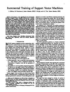
where χ[−,] is the characteristic function of the interval [−, ] and C is a normalization constant. Equations (14) and (15) arederived in the appendix. The shape of the functions in equations (14) and (15) is shown in figure (2). The above model has a simple interpretation: using the ILF is equivalent to assuming that the noise affecting the data is Gaussian. However, the variance and the mean of 1 ) has a unimodal the Gaussian noise are random variables: the variance (σ 2 = 2β distribution that does not depend on , and the mean has a distribution which is uniform in the interval [−, ], (except for two delta functions at ∓, which ensure that the mean is occasionally exactly equal to ∓). The distribution of the mean is consistent with the current understanding of the ILF: errors smaller than  do not count because they may be due entirely to the bias of the Gaussian noise.

a)

b)

1 Fig. 2. a) The probability distribution P (σ), where σ 2 = 2β and P (β) is given by equation 14 ; b) The probability distribution λ (x) for  = .25 (see equation 15).

5

Additional Results

While it is difficult to state the class of loss functions with an integral representation of the type (12), it is possible to extend the results of the previous section to a particular sub-class of loss functions, ones of the form:   h(x) if |x| <  V (x) = (16)  |x| otherwise,

where h(x) is some symmetric function, with some restriction that will become clear later. A well known example is one of Huber’s robust loss functions [5], for 2 which h(x) = x2 + 2 (see figure (3.a)). For loss functions of the form (16), it can be shown that a function P (β, t) that solves equation (12) always exists, and it has a form which is very similar to the one for the ILF. More precisely, we have that P (β, t) = P (β)λ (t), where P (β) is given by equation (14), and λ  (t) is the following compact-support distribution:  00 P (t) − P (t) if |t| <  (17) λ (t) = 0 otherwise,

where we have defined P (x) = e−V (x) . This result does not guarantee, however, 00 that λ is a measure, because P (t) − P (t) may not be positive on the whole interval [−, ], depending on h. The positivity constraint defines the class of “admissible” functions h. A precise characterization of the class of admissible h, and therefore the class of “shapes” of the functions which can be derived in this model is currently under study [7]. It is easy to verify that the Huber’s loss function described above is admissible, and corresponds to a probability t2 distribution for which the the mean is equal to λ  (t) = (1 + 1 − ( t )2 )e− 2 over the interval [−, ] (see figure (3.b)).

6

Conclusion and Future Work

An interpretation of the ILF for SVMR was presented. This will hopefully lead to a better understanding of the assumptions that are implicitly made when using SVMR. This work can be useful for the following two reasons: 1) it makes more clear under which conditions it is appropriate to use the ILF rather than the square error loss used in classical regularization theory; and 2) it may help to better understand the role of the parameter . We have shown that the use of the ILF is justified under the assumption that the noise affecting the data is additive and Gaussian, but not necessarily zero mean, and that its variance and mean are random variables with given probability distributions. Similar results can be derived for some other loss functions of the “robust” type. However, a clear characterization of the class of loss functions which can be derived in this framework is still missing, and it is the subject of current work. While we present this work in the framework of SVMR, similar reasoning can be applied

a)

a)

Fig. 3. a) The Huber loss function; b) the corresponding λ (x),  = .25. Notice the difference between this distribution and the one that corresponds to the ILF: while for this one the mean of the noise is zero most of the times, in the ILF all the values of the mean are equally likely.

to justify non-quadratic loss functions in any Maximum Likelihood or Maximum A Posteriori approach. It would be interesting to explore if this analysis can be used in the context of Gaussian Processes to compute the average Bayes solution. Acknowledgments Federico Girosi wish to thank Jorg Lemm for inspiring discussions.

References 1. T. Evgeniou, M. Pontil, and T. Poggio. Regularization networks and support vector machines. Advances in Computational Mathematics, 13:1–50, 2000. 2. F. Girosi. Models of noise and robust estimates. A.I. Memo 1287, Artificial Intelligence Laboratory, Massachusetts Institute of Technology, 1991. ftp://publications.ai.mit.edu/ai-publications/1000-1499/AIM-1287.ps. 3. F. Girosi. An equivalence between sparse approximation and Support Vector Machines. Neural Computation, 10(6):1455–1480, 1998. 4. F. Girosi, M. Jones, and T. Poggio. Regularization theory and neural networks architectures. Neural Computation, 7:219–269, 1995. 5. P.J. Huber. Robust Statistics. John Wiley and Sons, New York, 1981. 6. G.S. Kimeldorf and G. Wahba. A correspondence between Bayesian estimation on stochastic processes and smoothing by splines. Ann. Math. Statist., 41(2):495–502, 1971. 7. M. Pontil, S. Mukherjee, and F. Girosi. On the noise model of support vector machine regression. A.I. Memo 1651, MIT Artificial Intelligence Lab., 1998. ftp://publications.ai.mit.edu/ai-publications/1500-1999/AIM-1651.ps. 8. V. Vapnik. The Nature of Statistical Learning Theory. Springer, New York, 1995. 9. V. Vapnik, S.E. Golowich, and A. Smola. Support vector method for function approximation, regression estimation, and signal processing. In M. Mozer, M. Jordan, and T. Petsche, editors, Advances in Neural Information Processing Systems 9, pages 281–287, Cambridge, MA, 1997. The MIT Press.

10. V. N. Vapnik. Statistical Learning Theory. Wiley, New York, 1998. 11. G. Wahba. Splines Models for Observational Data. Series in Applied Mathematics, Vol. 59, SIAM, Philadelphia, 1990.

Appendix Proof of eq. 14 We look for a solution of eq. (12) of the type P (β, t) = P (β)λ(t). Computing the integral in equation (12) with respect to β, we obtain: Z +∞ dtλ(t)G(x − t, ) (18) e−V (x) = −∞

where we have defined:

G(t) =

Z

∞

dβP (β)

0

p

2

βe−βt .

(19)

Notice that the function G is, modulo a normalization constant, a density distribution, because both the functions in the r.s.h. of equation (19) are overlapping densities. In order to compute G we observe that for  = 0, the function e −|x| becomes the Laplace distribution which belongs to the model in equation (13). Then, λ=0 (t) = δ(t) and from equation (18) we have: G(t) = e−|t| .

(20)

Then, in view of the example discussed at the end of section 4.1 and equation (20), the function P (β) in equation (19) is: 1

P (β) = β 2 e− 4β , which (modulo a constant factor) is equation (14). To derive equation (15), we rewrite equation (18) in Fourier space: ˜  (ω), ˜ λ F˜ [e−|x| ] = G(ω)

(21)

sin(ω) + ωcos(ω) F˜ [e−|x| ] = , ω(1 + ω 2 )

(22)

with:

and: 1 . 1 + ω2 Plugging equation (22) and (23) in equation (21), we obtain: ˜ G(ω) =

(23)

˜ (ω) = sin(ω) + cos(ω). λ ω Finally, taking the inverse Fourier Transform and normalizing we obtain equation (15).