Numerical Heat Transfer, Part B, 40: 283± 301, 2001 Copyright # 2001 Taylor & Francis 1040-7790 /01 $12.00 + .00
ON THE NUM ERICAL IM PLEM ENTATION OF NONLINEAR VISCOELASTIC M ODELS IN A FINITE-VOLUM E M ETHOD Paulo J. Oliveira Departamento de Engenharia ElectromecaÃnica, Universidade da Beira Interior, CovilhaÄ, Portugal Numerical aspects of the implementation of nonlinear viscoelastic uid models in a nite volume method are investigated: (1) decomposition of the discretized stress equations in such a way that diagonal dominance is maximized, in order to promote numerical stability with iterative solvers; (2) imposition of boundary conditions for the stress components normal to a wall plane, and for pressure. These issues are investigated in relation to the Giesekus constitutive equation and illustrative ow examples showing the bene ts of the proposed methodology are given.
1. INTRODUCTION Solution of problems involving the ¯ ow of viscoelastic ¯ uids presents an extra degree of di culty, as compared to problems with Newtonian ¯ uids, in that the stress tensor components are new unknowns obeying their own governing di erential equations which must be solved simultaneously with the ¯ ow equations. The situation becomes, in a way, similar to the problem of solving turbulent Newtonian ¯ ows with Reynolds stress models of turbulence, in which one has to solve transport equations for the Reynolds stress components. In recent works [1, 2] we have imported and extended fairly standard ® nite-volume methods, used in computational ¯ uid dynamics (CFD) with Newtonian ¯ uids, to the solution of viscoelastic ¯ ow problems. We have used nonstaggere d meshes and generalized curvilinear coordinates, particularly suitable to represent complex ¯ ow geometries, and the methodology followed is in essence that described in great detail in the book by Ferziger and Peric [3]. In the work referred to above, we have considered only quasilinear constitutive models, and a number of numerical issues arise when the same methodology is applied to nonlinear models. In this article we consider the implementation of a typical nonlinear viscoelastic ¯ uid model, namely, the Giesekus [4] model, into an existing ® nite-volume method [1, 2]. This is a decoupled method in which the momentum and continuity equations are ® rst solved by means of a pressure-correction technique, with an assumed stress ® eld, and then the constitutive equations are solved sequentially for each stress component. In order to enhance the numerical stability of the procedure Received 21 December 2000; accepted 10 May 2001. Address correspondence to Dr. P. J. Oliveira, Universidade da Beira Interior, Departamento de Enga ElectromecaÃnica, 6200 CovilhaÄ, Portugal. E-mail:
[email protected] 283
284
P. J. OLIVEIRA
NOMENCLATURE aP ; aF B; Bf D Df De g( g_ ) H H(f) n p Re S ui ; S t ij S’tij t ti ; T i u; ui ; (u; v)
U v
coe cients in the discretized equations area (scalar or vector), cell-face surface area rate of deformation tensor [ˆ (Hu ‡ HuT )=2] Di usion conductance at cell face f (ˆ ZB=d) Deborah number (ˆ lU=H) model-dependent normal stress function half-width of channel operator in discretized equations normal (to wall) pressure Reynolds number (ˆ rUH=Z) source terms in the discretized momentum and stress equations additional nonlinear sources time component of stress vector (ti ˆ tij nj ) or force vector (T i ˆ Bf ti ) velocity vector and its Cartesian components (longitudinal, transversal) average velocity in channel cell volume
xi (x; y) a g_ d dt l m Z Z( g_ ) Z( g_ ) r xl s; tij
Cartesian coordinates (streamwise and cross-stream) parameter in Giesekus model shear rate normal distance to the wall time step relaxation time viscosity (Newtonian ¯ uid) viscosity parameter in viscoelastic model shear viscosity function viscosity ratio, Z( g_ )=Z density general coordinate extra stress tensor and its Cartesian components
Subscripts and Superscripts f cell face i; j; k Cartesian components (from 1 to 3) l directions along general coordinates (from 1 to 3) n; t normal and tangential components (relative to the wall) P; F generic control volume and neighbor (F from 1 to 6) special cell-face interpolation Ä ± linear interpolation H H upper convected derivative
it is advantageou s to deal implicitly with as many terms as possible in the solution of the constitutive equation, and the way to do this for a viscoelastic Giesekus ¯ uid is explained here. As far as we are aware, no other work has suggested a similar decomposition of the stress equation as that proposed here. Another important numerical issue associated with constitutive models which exhibit a normal stress component perpendicular to the main ¯ ow direction in rectilinear ¯ ow was found to be the implementation of boundary conditions. This question is especially relevant for the imposition of the normal stress at a solid wall and, as we shall show, an inadequate implementation leads to spurious oscillations of the velocity component normal to the wall. Past experience with the present ® nitevolume method (FVM) has been with models which have a vanishing normal stress at a wall [1, 2], such as the Newtonian, the upper-convecte d Maxwell (UCM) [5], and the Phan-Thien=Tanner (PTT) [6] models, and the problem of oscillating velocity ® elds did not emerge. Relevant work with the Giesekus model [4] has been presented by Lim and Schowalter [7], who derived the analytical solution in channel ¯ ow given as an implicit formula, followed by Choi et al. [8], who gave the explicit solution, with pro® les of velocity and stress as a function of the lateral coordinate. More recently, Azaiez et al. [9] presented the viscometric functions in a simple shear ¯ ow, and
NUMERICAL IMPLEMENTATION OF NONLINEAR VISCOELASTI C MODELS
285
we shall use their viscosity function to implement the boundary condition for the tangential stress at the wall. The normal stress will be obtained directly from the governing equations after imposing the appropriate approximations to the velocity components at the wall. In Section 2 the equations to be solved are given and their implementation in the FVM is explained for a general control volume (cell). Section 3 deals with the implementation of the boundary conditions for a cell adjacent to a wall. Flow examples illustrating the e ect of the issues discussed beforehand are given in Section 4. 2.
M ODEL IM PLEM ENTATION IN GENERAL
/
The governing equations are given ® rst in di erential form, and this is followed immediately by the discretized ® nite-volume equations, since the focus of the work is on numerical aspects of the solution method. The Giesekus model is given by the following constitutive equation: s‡ l t ‡
al s ¢ s ˆ 2ZD Z
(1)
to be solved for the extra stress tensor s, which is required in the momentum equation: r
Du ˆ ± Hp ‡ H ¢ t Dt
(2)
It is noted that the extra stress represents the part of the total stress which is related to ¯ uid motion but, for viscoelastic ¯ uids, pressure is not the only deviatoric part of the total stress. For incompressible ¯ ow, the continuity equation imposes a restraint on the velocity ® eld u, namely, H ¢u ˆ0
(3)
/
/
which is used to determine the pressure ® eld, p. In Eq. (1) the constant parameters l; Z, and a are the relaxation time of the ¯ uid, the viscosity coe cient, and a model parameter, respectively, and D is the rate-of-deformation tensor. D=Dt is the material derivative and the symbol is used to denote Oldroyd’s upper convected derivative, tˆ
Ds ± ( s ¢ H u ‡ H uT ¢ s) Dt
(4)
Following standard practices (Patankar [10], Ferziger and Peric [3]), the above di erential equations are integrated over control volumes (cells) in nonstaggered meshes, leading to algebraic linearized equations for momentum conservation, aP ui ˆ
6 X Fˆ1
aFuiF ‡ S ui -Dp ‡ S ui -stress ‡ S ui -diff ‡ S ui -other
(5)
P. J. OLIVEIRA
286
and for the stress evolution, atP tij ˆ
6 X Fˆ1
atFtijF ‡ S tij ‡ S’tij
(6)
The coe cients (aF and aP ) in these discretized equations account for convection and di usion contributions from the surrounding cells (F) to the cell in question (P, Figure 1a), and the source terms in the momentum equation (5) represent the pressure gradient S ui -Dp , the stress divergence term S ui -stress , a di usion contribution S ui -diff [which was added and subtracted to the original equation (2)] and other sources S ui -other (from the time-dependent term, boundary conditions, and possibly from use of high-resolutio n di erencing schemes). In the discretized constitutive equation the coe cients have only a convection contribution and the source term is conveniently split into two terms: that encompassing the linear terms in Eq. (1), and the nonlinear terms. If a ˆ 0 in Eq. (1), the UCM model is recovered, which is linear on the stress, and the implementation in a FVM follows that detailed in previous work [1]; so we need to pay attention only to the additional nonlinear term multiplied by a in Eq. (1). Since our method uses Cartesian components for both the velocity and stress ® elds, we can write that additional term after shifting it to the right-hand side of Eq. (1), where it acts as a source term [the source denoted with prime in Eq. (6)], under the following expanded form: al 2 (t ‡ t2xy ‡ t2xz ) Z xx al ± v (t2xy ‡ t2yy ‡ t2yz ) Z al ± v (t2xz ‡ t2yz ‡ t2zz ) Z al ± v (txx txy ‡ txy tyy ‡ txz tyz ) Z al ± v (txx txz ‡ txy tyz ‡ txz tzz ) Z al ± v (txy txz ‡ tyy tyz ‡ tyz tzz ) Z
S’txx ˆ ± v
(7a)
S’tyy ˆ
(7b)
S’tzz ˆ S’txy ˆ S’txz ˆ S’tyz ˆ
(7c) (7d) (7e) (7f)
In writing these equations we have used the fact that the stress is symmetric. v is the volume of the cell over which the equations have been integrated using the standard midpoint rule and, in the absence of a subscript, all quantities are evaluated at the center of the cell in question. We see from Eqs. (7) that the additional stress sources S’tij have terms proportional to the corresponding stress component (the tij in the identifying subscript of S’tij ), and these could be shifted to the left-hand side of the discretized stress equations where they would be incorporated into the main diagonal coe cient atP in order to enhance numerical stability. However, this operation requires two conditions:
NUMERICAL IMPLEMENTATION OF NONLINEAR VISCOELASTI C MODELS
287
Figure 1. Sketch of a general internal cell and a near-boundary (wall) cell.
1. The terms to be shifted to the left-hand side of Eq. (6) for promoting stability need to be always negative, so that they give a positive contribution to atP (it is well known, Patankar [10], that the coe cients of the discretized equation, aP and aF, need to be positive). 2. In addition, and with a view to end up with the same central coe cient atP for the six stress equations, those terms cannot be a function of any particular stress component (but may, of course, be a function of a stress invariant).
P. J. OLIVEIRA
288
The way to do this is not evident, unless we recognize that the trace of the extra stress tensor is always positive (tkk ² txx ‡ tyy ‡ tzz ¶ 0) and tends to be large in ``problematic’ ’ regions in a ¯ ow (singular-like regions, where stresses become very large, such as the region near a reentrant corner in a ¯ ow domain); see [11]. We may thus try to make explicit the negative terms on tkk in Eqs. (7), multiplied by the corresponding stress tij , and shift those terms to the left-hand side of the discretized equations. Since tkk is an invariant of the stress tensor, its incorporation into the central coe cient will not make this dependent on any particular stress component, or on the coordinate frame. This operation leads to the following modi® cation of the ``additional’’ stress sources and the atP coe cient: al 2 [t ‡ t2xz ± txx (tyy ‡ tzz )] Z xy al ± v [t2xy ‡ t2yz ± tyy (txx ‡ tzz )] Z al ± v [t2xz ‡ t2yz ± tzz (txx ‡ tyy )] Z al ± v (txz tyz ± txy tzz ) Z al ± v (txy tyz ± txz tyy ) Z al ± v (txy txz ± tyz txx ) Z
S’txx ˆ ± v
(8a)
S’tyy ˆ
(8b)
S’tzz ˆ S’txy ˆ S’txz ˆ S’tyz ˆ
(8c) (8d) (8e) (8f)
and atP ² atP ‡ v
al (t ) Z kk
(9)
The fact [Eq. (9)] that the central coe cient of the discretized stress equations is now much larger than in the original unmodi® ed equations [Eq. (6)], besides promoting numerical stability in the overall iterative method, brings the bene® t of stronger diagonal dominance, and so the performance of the iterative solvers will be improved. 3.
IM PLEM ENTATION OF BOUNDARY CONDITIONS
3.1. For St resses In [7, 8] it is shown that the Giesekus model has a nonvanishing normal stress tyy in a channel ¯ ow aligned with direction x. The presence of such transversal normal stress, which are absent in the quasi-linear UCM and Oldroyd-B models [5], is a cause of some numerical trouble, especially in relation to the imposition of boundary conditions at a solid wall, and this is now discussed. For a Newtonian ¯ uid it is straightforward to show that the normal stress at the channel wall (y ˆ H), tyy ˆ 2m qv=qy, is zero because at the wall u ˆ v ˆ 0 and continuity, qu=qx ‡ qv=qy ˆ 0, implies qv=qy ˆ 0. For the Giesekus model this is not
NUMERICAL IMPLEMENTATION OF NONLINEAR VISCOELASTI C MODELS
289
the case, and from integration of the stress-divergence term in Eq. (2) we obtain, in general (i.e, valid for any rheological model and wall orientation), a contribution to the i-momentum equation given by S ui ˆ Bf ti
(10)
where Bf is the scalar surface area [m2 ] of a cell face coinciding with the wall (see Figure 1b), and ti is the force component per unit area (the tension vector). This force can be decomposed into a tangential and a normal component as ti ˆ tti ‡ tni
(11)
The ¯ ow adjacent to the wall is viscometric and the tangential component of the stress vector is determined from tti ˆ Z( g_ )
quti qn
(12)
where n is the normal to the wall and Z( g_ ) denotes the shear viscosity function, which depends on the local shear rate g_ . It is noted that although Z is a constant parameter of the model, Z( g_ ) is a decreasing function of g_ for a shearthinning ¯ uid as that simulated by the Giesekus model. For the UCM model Z( g_ ) is constant and coincides with ZÐ it is a constant viscosity model, sometimes called a Boger ¯ uid; the Newtonian ¯ uid has a constant viscosity as well (if dependence on temperature is not considered), usually denoted m, instead of Z. In the discretized equation for cell P adjacent to the wall (Figure 1b), Eq. (12) is written as (tti ) f ˆ [Z( g_ )]f
Á ! utif ± utiP
(13)
df
where df is the distance from f to cell center P along the normal to the wall, and utif ² uif is the wall velocity (for a stationary wall, uif ˆ 0). The tangential velocity component at the cell center P is obtained from
uiP ˆ uniP ‡ utiP ) utiP ˆ uiP ± uniP ˆ uiP ±
Á
X j
!
ujP nj ni
(14)
where ni is the unit vector component of the normal to the wall. For the Giesekus model, and according to Azaiez et al. [9], we have 2
n( g_ ) ˆ Z
(1 ± o) 1 ‡ (1 ± 2a)o
(15)
P. J. OLIVEIRA
290
with
oˆ
1± L 1 ‡ (1 ± 2a)L
2
6 Lˆ4
and
31=2
2 7 q 5 2 1 ‡ 1 ‡ 16a(1 ± a)(lg_ )
and the shear rate g_ at the wall node f can be obtained numerically as either g_ f ˆ
uif ± utiP ² g_ w1 df
(16)
or g_ f ˆ g_ P ² g_ w2
(17)
p with g_ P calculated as for any internal cell, i.e., g_ P ˆ 2D ij D ij (twice the square root of the second invariant of the deformation rate tensor). The merits of these choices for the wall shear rate will be discussed in Section 4. For implementation of the force on the wall cell-face surface we recall the method described in [1], where terms resulting from stress divergence are inserted explicitly in the momentum equation [source term S ui ± stress in Eq. (5)] and an ordinary di usion term is added and subtracted [S ui ± diff in Eq. (5)]. For the near-wall cell, the momentum equation is written as aP uiP ˆ H(ui ) ‡ aF(uiF ± uiP ) ± aF(uiF ± uiP ) ‡ T if
(18)
P where the operator H(ui ) ² aFuiF ‡ S ui incorporates all terms not related to the boundary face f, and T if ˆ Bf (ti ) f is the force applied at that cell face. In the absence of convective ¯ uxes through the wall, the aF coe cient in the underlined term is given by aF ˆ D f ² Bf Zf =df , being a standard di usion conductance, and it is treated implicitly. This implies that this term is shifted to the left-hand side and the equation becomes (aP ‡ D f )uiP ˆ H(ui ) ‡ D f uiP ‡ T if
(19)
where the new underlined term is the wall-related source term, S uif . For a Newtonian ¯ uid, neglecting the normal stress component (which is zero in the di erential equations) , we have T f i ˆ B f mf
quti qn
f
º
Bf m f (utif ± utiP ) ’ df
(20)
and for the case of negligible or small mesh skewness near the wall (uiP º uiP’ , Figure 1b), the wall source term, from Eqs. (19), (20), and (14), becomes
NUMERICAL IMPLEMENTATION OF NONLINEAR VISCOELASTI C MODELS
"
S uif ˆ D f uif ‡
Á X j
! #
ujp nj ni ˆ D f (uif ‡ unP ni )
291
(21)
For a viscoelastic ¯ uid in general, in addition to the tangential stress given by the same expression as above (Eq. 20), but where the viscosity (m or Z) is now variable Z( g_ ), there is a normal stress component which can be written as tn ˆ ± g( g_ )lZg_ 2
(22)
with the function g( g_ ) speci® c for each model. A manipulation similar to the above leads now to S uif ˆ D f [uif ‡ (1 ± Zf )(uiP ± uif ) ‡ ni (Z Zf unP § g( g_ f )ldf g_ 2f )]
(23)
In this expression the di usion conductance D f is still based on the constant viscosity coe cient Zf (so D f ˆ Zf Bf =df ) and the shear-thinning e ect is accounted for by the viscosity ratio Zf ˆ Z( g_ f )=Zf . So, in general, Zf will be smaller than 1, except for the UCM or Newtonian ¯ uid, in which case Zf ˆ 1 and the above expression for the wall source becomes equal to that given before, Eq. (21). When the wall is placed along the positive xf direction, as in Figure 1b, the minus sign in the § of Eq. (23) is used; otherwise, for a wall in the negative xf direction, it is the plus sign that is used. For the Giesekus model the g( g_ ) function in Eq. (22) is obtained from the analytical solution. The constitutive equation normal to the wall, tyy , reduces to al 2 al 2 tyy ‡ tyy ‡ t ˆ0 Z Z xy
(24)
with txy ˆ Z( g_ ) g_ . The only physically relevant solution to this quadratic equation for tyy is tyy ˆ
2 (± 2al=Z)Z( g_ ) g_ 2 q 1 ‡ 1 ± 4(al=Z) 2 Z( g_ ) 2 g_ 2
(25)
which has been written in a convenient form to recover the appropriate limits for the UCM or Newtonian ¯ uids, whenever a or l go to zero. Now, comparison with Eq. (22) gives the de® nition of g( g_ ) as 2
g( g_ ) ˆ
2aZ Z( g_ ) q 1 ‡ 1 ± 4(al) 2 Z( g_ ) 2 g_ 2
(26)
3.2. For Pressure At this point we have appropriate stress-related boundary conditions at the wall. However, the use of the nonstaggered mesh arrangement implies the need to
P. J. OLIVEIRA
292
specify boundary conditions for pressure as well. By looking at Figure 1, we see that the momentum balance along the wall direction xf gives rise to a term proportional to the pressure di erence (DP) f;P ˆ pf ± pf ± and therefore the pressure at the wall, pf , is required. In CFD with Newtonian ¯ uids the accepted practice (Ferziger and Peric [3]) has been to extrapolate linearly pressure from adjacent internal cells to the wall, and this practice has worked well. In viscoelastic ¯ ow computations with ¯ uids exhibiting strong normal stresses perpendicular to the wall, we found that pressure extrapolation is not satisfactory (see results in Section 4). A better formulation can be derived from the momentum equation normal to the wall at the interior point P, aP unP ˆ [H(u)]P ± BnP ( pf ± pf )
(27)
[the H operator here di ers from that in Eq. (18)] and the corresponding equation for the cell face velocity obtained with the Rhie-Chow [12] interpolation is aP u~ nf ˆ [H(u)]P ± Bf ( pf ± pf ± )
(28)
In Eqs. (27) and (28), aP is the central coe cient for the discretized momentum equation, H(u) is an operator contabilizing transport e ects from surrounding cells and source terms except for the normal pressure gradient, and the overbar denotes arithmetic averaging. Since the ``cell’’ surrounding the cell face point at the wall, f, can be imagined as of zero thickness, we have aP ˆ aP =2 and H(u) ˆ H(u) P =2. From the impermeable condition ( u~ nf ˆ 0), and by assuming that the nonorthogonalit y of the adjacent cell is not too severe (BnP º Bf , the cell face area), we obtain for the value of pressure at the wall: pf ˆ
aP unP ‡ 2pP ± pf Bf
(29)
Thus we see that an extra term appears, in addition to the linearly extrapolated value. Since in the momentum equation we only need the pressure di erence normal to the wall, and that di erence based on an extrapolate d value was already implemented, the only modi® cation required is [Dp]nP ˆ [Dp]nP lin:extrap: ‡ 4.
aP unP Bf
(30)
ILLUSTRATIVE RESULTS
The previous ideas are ® rst illustrated with a simple, although not trivial, ¯ ow problem. We consider the ¯ ow of a Giesekus ¯ uid with model parameter a ˆ 0:5 along a straight channel aligned with the x axis. For reasons of symmetry, only the upper part of the channel is taken as ¯ ow domain, with symmetry conditions imposed at y ˆ 0, a solid wall with no-slip conditions at y ˆ H (H is half-channel width), inlet at x ˆ 0, and outlet at x ˆ L (L ˆ 10H). In the present problems the outlet plane was su ciently far away from regions of interest and the ¯ ow had
NUMERICAL IMPLEMENTATION OF NONLINEAR VISCOELASTI C MODELS
293
almost recovered to a unidirectional, fully developed state so that simple outlet boundary conditions were deemed adequate, with imposed zero streamwise gradients for velocity, stress, and pressure gradients: qu=qx ˆ qt=qx ˆ qHp=qx ˆ 0. At the inlet plane we prescribe fully developed conditions corresponding to a UCM ¯ uid at the same Reynolds (Re ˆ rUH=Z) and Deborah (De ˆ lU=H) numbers, both taken
Figure 2. Channel £ow of the Giesekus £uidöcomparison with theoretical results for De ˆ 1: (a) velocity pro¢le ; (b) stress pro¢les (tx x ; tyy ; tx y ).
294
P. J. OLIVEIRA
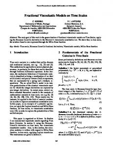
as unity. We recall that the fully developed velocity and shear stress (txy ) pro® les for a UCM ¯ uid are identical to those of a Newtonian ¯ uid (being parabolic and linear, respectively), but it also presents a nonvanishing axial normal stress (txx ). All computations have been performed in double precision, and iterative convergence was assumed when the normalized residuals for all equations (including the stress equations) fell below a precribed tolerance of 10 ± 4 . Because these imposed pro® les at the inlet di er signi® cantly from the fully developed conditions of the Giesekus ¯ uid, a developing region will be established before the ¯ uid reaches those fully developed conditions. At stations near the outlet, ¯ ow development is expected to be completed, and this is borne out in a comparison between predictions and the theoretical solution (Figure 2). In this ® gure we see that both the axial velocity and the three nonzero stress pro® les are perfectly predicted by the numerical calculations, on a uniform mesh with 20 (axial)6100 (lateral) control volumes. A detail of the streamlines in a region close to inlet (spanning from x ˆ 0 to x ˆ 3H) shows that the ¯ ow there is not a rectilinear simple ¯ ow, and even shows signs of a small recirculation (Figure 3). The purpose of this ® gure is to demonstrate that the present test problem possesses some complexity in the region near the inlet, due to the imposed inlet conditions. This ® gure also shows the contours of the axial
Figure 3. Streamlines and normal stress contours (txx ) for the developing channel £ow of the Giesekus £uid (detail near inlet).
NUMERICAL IMPLEMENTATION OF NONLINEAR VISCOELASTI C MODELS
295
Figure 4. Pro¢le of the predicted lateral velocity component (v) with two boundary conditions for pressure: linear extrapolation and Eq. (30).
normal stress component [T xx ˆ txx =(ZU=H)], which tend to a uniform (in x) lateral variation as one moves away from inlet. Figure 4 shows a pro® le of the lateral velocity component at the last station before the outlet, and serves to illustrate the bene® cial e ect of the modi® ed pressure boundary condition discussed in Section 3 [Eq. (30)]. The simple linear extrapolation of pressure to the wall boundary face gives rise to small oscillations seen in the ® gure (a zoomed view is included to help observation); these are surpressed with the
Figure 5. Comparison of theoretical and numerical pro¢les of the shear rate g_ , and e¡ect of using a wall shear rate given by Eq. (16) or (17) in determining the viscosity function Z( g_ ).
296
P. J. OLIVEIRA
Figure 6. Sketch of the geometry for the entry £ow problem.
modi® ed pressure boundary condition given by Eq. (30). With coarser meshes, these oscillations would tend to become more pronounced. Figure 5 shows a theoretical fully developed pro® le of the rate of deformation g_ for the Giesekus ¯ uid with a ˆ 0:5, and numerical predictions obtained in a mesh with 20 cells across the channel. Two predictions are shown: in one (marked gw1 ), the g_ values used to impose the boundary condition at the wall are based on Eq. (16), and in the other (marked gw2 ), they are given by Eq. (17). Clearly, when the wall value of g_ is approximated by a simple di erence between tangential velocity components at the cell center P and the wall velocity (here equal to zero), divided by the corresponding distance, much better results are obtained compared with the zeroorder approximation g_ w ˆ g_ P (with g_ P calculated as for the internal cells). Similar perturbations (not shown here) are obtained in the stress pro® les, since these depend on g_ . The ® gure is also useful in showing that, even for the relatively low De con-
Figure 7. Streamlines in the zone from x ˆ ± 0:5H to ‡1:5H , around the singular point, for De ˆ 0 (Newtonian solid lines), 1 (short dashes), and 2 (long dashes).
NUMERICAL IMPLEMENTATION OF NONLINEAR VISCOELASTI C MODELS
297
Figure 8. Contours of the normal stress ¢eld at De ˆ 2.Values are normalized with ZU =H . (a) tx x ; (b) tyy .
sidered (De ˆ 1), there is a very steep increase of g_ in a thin layer adjacent to the wall, and as De is increased, ® ner meshes will be required in order to avoid oscillations. As a second test case we consider an entry ¯ ow, sketched in Figure 6, where a freely ¯ owing stream (between two symmetry planes) is forced into a plane channel (symmetry plane and wall separated by a distance H). This is known [1, 13] to be a more di cult problem (in numerical terms) because the point at x ˆ 0 and y ˆ H, where the boundary condition changes from pure slip (x µ 0) to no-slip (x > 0), is a singular point with stresses locally tending to in® nity. An inverse problem, known as the stick-slip problem, is often used as a comparison test case in
298
P. J. OLIVEIRA
Figure 9. Pro¢les of the axial velocity component for De ˆ 2, at positions x=H ˆ1, 2, and 3 (downtream of singular point).
viscoelastic ¯ ow calculations (e.g., [14, 15]). The entry ¯ ow problem o ers some advantage in that the inlet conditions are easier to imposeÐ in fact, they consist only of a uniform axial velocity pro® le and zero stressesÐ and another reason for using this same simple geometry is that it has been used in a previous work [1] with the UCM ¯ uid. For the present calculations with the Giesekus ¯ uid (a ˆ 0:5) we have utilized a relatively ® ne mesh with 2506100 nonuniform cells (® ner than that in [1]) at a Reynolds number of unity. A discussion of accuracy and e ects of mesh re® nement is given below, at the end of this section. Figure 7 shows the resulting streamlines in a zoomed view around the point where the boundary conditions change, for three cases: De ˆ 0 (Newtonian), 1, and 2. As De increases, the ¯ ow at the entrance to the channel tends to go straight for a longer distance and it is curved upward, toward the singular point, because the local high shear rates decrease the viscosity. Farther downstream into the channel, the ¯ ow is then de¯ ected downward, as a result of the elastic stresses developed around the singular point (see discussion in [1]). These ¯ ow patterns are in contrast to those observed in [1] for the constant-viscosit y ¯ uid, where the important e ect was the downward de¯ ection due to elasticity. The corresponding contours of the axial and transversa l normal stresses at De ˆ 2 are shown in Figure 8, where they are seen to be smooth. Maximum values of txx and tyy , normalized by ZU=H, are 43.8 and 2.6, respectively, compared with 0.78 and 16.9 for De ˆ 0. Because of strong shear thinning, the Giesekus ¯ uid forms a thin boundary layer adjacent to the top wall in the channel. This is evident in the plot of the velocity pro® les at several axial positions (x=H ˆ 1, 2, and 3) given in Figure 9. For higher elasticity and in complex geometries, the resolution of such thin boundary layers requires adoption of special procedures which are under investigation.
NUMERICAL IMPLEMENTATION OF NONLINEAR VISCOELASTI C MODELS
299
Figure 10. E¡ect of mesh re¢nement on predicted velocity pro¢les (case De ˆ 1): (a) at x=H ˆ 1,with three meshes; (b) at x=H ˆ 2, with two meshes. Also shown is a pro¢le at outlet (x=H ˆ 10), and the theoretical solution for fully developed £ow.
In viscoelastic ¯ ow problems with singular points it is notoriously di cult to accomplish grid independence because the ® ner the grid, the higher the predicted stresses on grid nodes near the singular point; those high stresses are then convected downstream by the Oldroyd-derivativ e terms in the constitutive equation.
P. J. OLIVEIRA
300
Figure 10 shows, for the ¯ ow case De ˆ 1, the e ect of grid re® nement on the predicted velocity pro® les at two positions, situated at 1 and 2 half-widths downstream of the singular point (inside the channel). Two nonuniform grids have been used: one is the ® ne mesh used above (25,000 cells), and the other is a medium mesh (6,250 cells) having half the resolution of the ® rst; the minimum controlvolume spacing of these meshes was 0.005H and 0.01H, respectively. That mesh spacing expands from the singular point at a constant rate of 1.83% and 3.69% axially, and 1.27% and 2.56% laterally, for the two meshes. The ® gure shows that the results from the two meshes are already very close for the pro® le at x ˆ 2H, but some di erences are still seen for the velocity pro® le closer to the problematic singular point. Results from an initial uniform mesh with constant spacing of dx ˆ 0:1H and dy ˆ 0:01H (20,000 cells) are also given in Figure 10a (referred to as ``uniform’ ’ mesh), but in spite of the high number of cells the resolution is similar to that achieved with the medium mesh. As an additional check, Figure 10b also compares the velocity pro® le at x ˆ 10H with the theoretical fully developed solution, and perfect agreement is observed. This clari® es the adequacy of the imposed outlet boundary condition for the present simulations. Further related details on the issue of accuracy can be obtained from [1]. 5.
CONCLUSIONS
The numerical implementation in a ® nite-volume method of a nonlinear viscoelastic ¯ uid model, the Giesekus ¯ uid, is discussed. The Giesekus model is one of the constitutive equations often used for elastic ¯ uids exhibiting shear thinning (decrease of viscosity with shear rate), but the numerical aspects of the work are valid for other nonlinear models. Two points are investigated: how to incorporate the additional nonlinear terms of the constitutive equation into the scheme in such a way that numerical stability is promoted; and how to introduce boundary conditions in such a way that oscillations are avoided. Results from a developing channel ¯ ow case are compared with theoretical solution for fully developed conditions, and serve to justify the proposed implementation. Another example considered is that of an entry ¯ ow into a channel, a case which has a singular point where stresses tend to in® nity, and thus poses a more severe test to the method. Smooth streamlines and stress contours are achieved. REFERENCES 1. P. J. Oliveira, F. T. Pinho, and G. A. Pinto, Numerical Simulation of Non-Linear Elastic Flows with a General Collocated Finite-Volume Method, J. Non-Newtonian Fluid Mech., vol. 79, pp. 1± 43, 1998. 2. P. J. Oliveira and F. T. Pinho, Numerical Procedure for the Computation of Fluid Flow with Arbitrary Stress-Strain Relationships, Numer. Heat Transfer B, vol. 35, pp. 295± 315, 1998. 3. J. H. Ferziger and M. PericÂ, Computational Methods for Fluid Dynamics, Springer-Verlag, Berlin, 1996. 4. H. Giesekus, A Simple Constitutive Equation for Polymer Fluids Based on the Concept of the Deformation Dependent Tensorial Mobility, J. Non-Newtonian Fluid Mech., vol. 11, pp. 69± l09, 1982.
NUMERICAL IMPLEMENTATION OF NONLINEAR VISCOELASTI C MODELS
301
5. R. B. Bird, R. Armstrong, and O. Hassager, Dynamics of Polymeric L iquids, V ol. 1, Fluid Mechanics, 2d ed., Wiley, New York, 1987. 6. N. Phan-Thien and R. I. Tanner, A New Constitutive Equation Derived from Network Theory, J. Non-Newtonian Fluid Mech., vol. 2, pp. 353± 365, 1977. 7. F. J. Lim and W. R. Schowalter, Pseudo-spectral Analysis of the Stability of PressureDriven Flow of a Giesekus Fluid between Parallel Plates, J. Non-Newtonian Fluid Mech., vol. 26, pp. 135± l42, 1987. 8. H. C. Choi, J. H. Song, and J. Y. Yoo, Numerical Simulation of the Planar Contraction Flow of a Giesekus Fluid, J. Non-Newtonian Fluid Mech., vol. 29, pp. 347± 379, 1988. 9. J. Azaiez, R. GueÂnette, and A. Ait-Kadi, Numerical Simulation of Viscoelastic Flows through a Planar Contraction, J. Non-Newtonian Fluid Mech., vol. 62, pp. 253± 277, 1996. 10. S. V. Patankar, Numerical Heat T ransfer and Fluid Flow, Hemisphere, Washington, DC, 1980. 11. P. J. Oliveira, A Traceless Stress Tensor Formulation for Viscoelastic Fluid Flow, J. NonNewtonian Fluid Mech., vol. 95, pp. 55± 65, 2000. 12. C. M. Rhie and W. L. Chow, A Numerical Study of the Turbulent Flow past an Airfoil with Trailing Edge Separation, AIAA J., vol. 21, pp. 1525± 1532, 1983. 13. C. D. Eggleton, T. H. Pulliam, and J. H. Ferziger, Numerical Simulation of Viscoelastic Flow using Flux Di erence Splitting at Moderate Reynolds Numbers, J. Non-Newtonian Fluid Mech., vol. 64, pp. 269± 298, 1996. 14. M. R. Apelian, R. C. Armstrong, and R. A. Brown, Impact of the Constitutive Equation and Singularity on the Calculation of the Stick-Slip Flow: The Modi® ed Upper-Convected Maxwell Model (MUCM), J. Non-Newtonian Fluid Mech., vol. 27, pp. 299± 321, 1988. 15. S. Richardson, Proc. Camb. Phil. Soc., vol. 67, pp. 477± 489, 1970.