to continue processing, the data provided by hard disk will be discarded. ... With probability 1âγ it is necessary to wait for the hard disk to deliver the data, ...... recovery in manufacturing systems control. ... Technical Report Project MAC Tech.
On the performance evaluation of multi-guarded marked graphs with single-server semantics∗ Jorge J´ulvez† Jordi Cortadella Universitat Polit`ecnica de Catalunya Barcelona, Spain
Michael Kishinevsky Intel Corporation Hillsboro, USA
Abstract In discrete event systems, a given task can start executing when all the required input data are available. The required input data for a given task may change along the evolution of the system. A way of modeling this changing requirement is through multi-guarded tasks. This paper studies the performance evaluation of the class of marked graphs extended with multi-guarded transitions (or tasks). Although the throughput of such systems can be computed through Markov chain analysis, two alternative methods are proposed to avoid the state explosion problem. The first one obtains throughput bounds in polynomial time through linear programming. The second one yields a small subsystem that estimates the throughput of the whole system.
Keywords: Early evaluation, throughput bounds, Petri nets, marked graphs.
1 Introduction The modeling of discrete event systems often relies on a producer/consumer pattern. According to this pattern, a given consumer action cannot start until all the required input items have been produced by some previous producer actions. For example, in a digital circuit an adder that computes the sum of two integer numbers cannot start operating until both numbers are available at the input of the adder. Nonetheless, there are actions that do not always require all its input data to be available to start operating. A typical component exhibiting this behavior is a multiplexer. A multiplexer is a device that selects one of many input channels and outputs the value of that channel. The values of the rest of the channels are useless. Hence, a multiplexer could start operating as soon as the value of the selected channel is available without waiting for the rest of the values. The availability of the selected channel is the precondition, or guard, required by the multiplexer to start working. Given that different input channels may be selected along time, the multiplexer guard is not constant but changes along time. Consider a computer program that processes the data records of a given file stored in a hard disk. In order to speed up the program execution, some fields of the records are stored in memory. Let us assume that with probability γ the program just requires the fields stored in memory to process a record, and with probability 1 − γ it requires ∗ This
work has been partially supported by a gift from Intel Corp. and CICYT TIN 2004-07925. by the Spanish Ministry of Education and Science (Juan de la Cierva fellowship) and by the European Communitys Seventh Framework Programme under project DISC (Grant Agreement n. INFSOICT-224498). † Supported
1
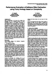
all the fields of the record. Once a data record is processed, the program requests a new record. Such request activates two actions in parallel: one searches the record in the memory and the other one in the hard disk. If the fields stored in memory are sufficient to continue processing, the data provided by hard disk will be discarded. The behavior of this system can be modeled by a Petri net, see the net S1 in Figure 1. The transitions (bars) of the system represent actions that consume the tokens (black dots) stored in the input places (circles), and after completion, store new tokens in the output places (see [Mur89, Sil93] for a tutorial on Petri nets). The token in place p1 describes the situation in which a record has just been processed and that a new record is to be requested. Once the request is issued, the token from p1 is removed, a token is placed in p2 , and a token is placed in p4 : accessing memory and hard disk is being done in parallel. Getting record fields from memory just needs one task, Memory, after which memory fields are ready to be processed. Getting the whole record from hard disk needs three tasks: Access, Search and Deliver. With probability γ, memory fields are enough to continue processing, and therefore, the data provided by disk will be ignored. Hence, the Process action not only processes data, but acts as a multiplexor by selecting either the memory fields or the whole record. It will be assumed that all tasks last the same amount of time. Memory
S1
p4
p2 p5
p3
p7
p6
p1
Request
Process Access Search
Deliver
S2
S3
1−γ
S5
γ S4
S6 −1
Figure 1: Reachable states of an early evaluated system that processes data records of a file stored in a hard disk.. The graph in Figure 1 depicts the set of reachable states. A directed arc connects a given state to a successor state. Arcs are labeled with the probability of being taken. If the probability of taking the arc is 1, the label is omitted. Let us focus on state S3 at which memory fields are already available but the hard disk has not provided yet all fields. With probability 1 − γ it is necessary to wait for the hard disk to deliver the data, i.e., the path (S3, S5, S6) is taken. At S6 all data is available and can be processed. When moving from S6 to S1 the tokens in p3 and p7 are consumed (although only the one is p7 is required) and a new token in p1 is put meaning that a new request must be done. On the other hand, from S3 there is a probability γ of not having to wait for the 2
disk, i.e., the arc from S3 to S4 is taken. In such case, the memory fields are processed (the token in p3 is consumed) and a new record request is issued (a token in p1 is put). Notice that in parallel to this processing, the disk is working in order to get the whole record which must not be processed. A simple way of discarding the token that will be delivered by the Deliver task is by putting a negative token in p7 at S4. This way, the token that will produce the Deliver task at p7 will vanish when meeting the negative token, state S2. The main new feature of the model in Figure 1, with respect to conventional Petri nets, is that it is not strictly necessary to finish every previous task before starting the Process task. This fact provides more flexibility to the modeling of discrete event systems and usually increases the system performance (if Process is executed only after Memory and Deliver, the system state will loop on S1, S2, S3, S5 and S6, ignoring the short cut provided by S4). A natural consequence of performing a task, like Process, without having finished some previous tasks, Deliver, is that negative tokens appear after the completion of the task, state S4. Negative tokens are necessary to be consistent with the producer/consumer pattern, in which a token is consumed from every input place. Moreover, they have the responsibility of getting rid of non required tokens, like the token in place p7 at S4. Negative tokens have been considered in several works for different purposes. In [MY90], Petri nets with negative tokens are used to study automated reasoning programs. Negative event graphs are introduced in [LP05] to analyze time window constraints. In [OM05], a negative token represents a temporary buffer overflow in a manufacturing system. Differential places of differential Petri nets [DK98] are allowed to store real quantities (positive or negative) of tokens in order to model hybrid systems.
1.1 Framework and Contribution This paper focuses on the class of Multi-Guarded Marked Graphs (GMG). The underlying structure of a GMG is that of a conventional marked graph (MG), a Petri net subclass that offers an interesting trade-off between modeling power and analysis capability [Mur89]. In contrast to conventional MGs, a transition of a GMG can have several guards, i.e., it is multi-guarded, which are randomly selected. With respect to the preliminary results obtained in [JCK06], the present paper discusses the boundedness property of GMGs, analyzes the resulting throughput bounds, and proposes a heuristics to improve the obtained throughput bounds. The main goals of the paper are the following: • Provide an efficient method to compute steady state throughput bounds. • Describe a heuristics to obtain a small subsystem that estimates the steady state throughput. Before focusing on these goals, essential system properties as liveness and boundedness of GMGs are studied to ensure the well-behavior of the system. The approach suggested in this paper to compute steady state throughput bounds is based on Linear Programming (LP). Such an approach allows us to naturally manage structural and steady state constraints of GMG. LP techniques have been intensively used to compute throughput bounds in the framework of queueing networks and Petri nets. In the queueing network setting, some representative works in the literature are the following: [KK94] establishes a set of linear equality constraints on the mean values of some variables and conservation laws
3
allow to bound the performance of the system. A similar approach is taken in [BC99], where the region of achievable performance vectors is characterized in order to formulate a linear programming problem to obtain bounds. In [YCT84], performance bounds for bulk arrival queues are computed by making use of the bounds for single arrival queues. In the Petri nets framework (notice that with respect to queueing networks, Petri nets include a synchronization primitive), two main approaches that make use of LP techniques can be distinguished. In [Liu98], the uniformization technique is used to derive linear equalities and then LP is applied to obtain throughput bounds. In [CAC+ 95, CS92], the use of operational laws allows one to obtain linear constraints that are included in a LP problem whose solution is an upper bound for the throughput. Similarly to [KK94, BC99], the approach presented here establishes some linear constraints related to conservation laws and mean values of throughput and average markings [CS92] to design a Linear Programming Problem (LPP). The solution of the LPP is an upper bound for the throughput in the steady state. In contrast to previous approaches, in order to handle multi-guarded transitions, a new expression relating the throughput and average marking of multi-guarded transitions has been developed and included in the mentioned LPP. With respect to the second goal, the heuristics is based on obtaining a small subsystem whose throughput is similar to the throughput of the whole system. The subsystem is built from the solution obtained by a LPP and an iterative process. As far as we know, no similar approach has been proposed before in the literature. The rest of the paper is organized as follows: Section 2 defines the class of MultiGuarded Marked Graphs (GMG) and presents some basic properties. Section 3 shows how to compute the throughput of a GMG by using Markov chains. Section 4 presents a linear programming problem to compute upper bounds for the throughput. A procedure to obtain a small bottleneck subsystem of a GMG is explained in section 5. Section 6 shows the obtained experimental results. Conclusions are drawn in section 7.
2 Multi-Guarded Marked Graphs 2.1 Definition and Semantics In the following, the reader is assumed to be familiar with Petri nets (PN s) (see [Mur89, Sil93] for a tutorial on Petri nets). Definition 1 (GMG) A
Multi-Guarded
Marked
Graph
(GMG)
is
a
tuple
N = hP, T, Pre, Post, G, m0 i where: • P is a finite set of places, and T is a finite set of transitions. The preset and postset of a node x ∈ P ∪ T are denoted as • x and x• . The following condition holds: ∀p ∈ P, |• p| = |p• | = 1. • Pre : P × T → N ∪ {0} and Post : P × T → N ∪ {0} are the pre- and post- incidence functions that specify the arc weights. The incidence matrix of the net is C = Post − Pre. P
• G : T → 22 assigns a set of guards to every transition. The following conditions must be satisfied: a) ∀ g ∈ G(t) it holds g ⊆ •t; b) ∪ g = •t. g∈G(t)
• m0 : P → N ∪ {0} is the initial marking.
4
A conventional Marked Graph (MG) is simply a GMG in which G(t) = {{•t}} for every t ∈ T . In a GMG, the transitions can also satisfy the condition G(t) = {{•t}}. Such transitions will be called simple transitions, the rest of transitions will be called multi-guarded transitions. Simple transitions will be represented graphically as empty rectangles; multi-guarded transitions will be represented as rectangles with oblique lines inside (see Figure 2 for a multi-guarded transition). Definition 2 (Firing semantics) The dynamic behavior of a GMG system is determined by its firing rules. The execution of a transition t can be described as follows: • Guard selection. A guard g(t) ∈ G(t) for the next firing is selected nondeterministically. The guard selection is trivial for simple transitions, since they only have one guard. For multi-guarded transitions any guard in G(t) can be selected. The selected guard of a transition t is persistent, i.e., it does not change until t fires. • Enabling. If the guard g(t) ∈ G(t) has been selected for the next firing of t, then the transition t becomes enabled when every place p ∈ g(t) is positively marked, i.e., m(p) > 0. • Firing. A transition t enabled at marking m can fire leading to marking m′ such that m′ = m + C(P,t) where C(P,t) is the column of C corresponding to t. Notice that GMGs can reach markings with negative values. If m(p) ≥ 0 one says that place p has m(p) positive tokens. Otherwise, place p has |m(p)| negative tokens. Negative tokens account for the data that must be discarded when arriving at the input of the transition. As in conventional MGs the state equation m = m0 + C · σ provides a necessary condition for the reachability of m, where σ is the firing count vector of the transitions and m can contain negative elements. Then, vectors y ≥ 0, y · C = 0 (x ≥ 0, C · x = 0) represent P-semiflows or conservative components (T-semiflows or consistent components). A semiflow v is said to be minimal when its support, kvk, is not a proper superset of the support of any other, and the greatest common divisor of its elements is one. As in conventional MGs [Mur89], every minimal P-semiflow of a GMG corresponds to a simple cycle, i.e., a cycle with no repeated vertices except for the start and end vertex. Example 1 Let us assume that the transition in Figure 2 has two guards G(t) = {{pa , pb }, {pa , pc }}, and that initially the places pa and pc have a token.
pa
pb
pc
pa
pb −1
pc
pa
g = {pa , pc }
pb
pc
pa
pb
pc
g = {pa , pb }
(a)
(b)
Figure 2: Multi-guarded transition: (a) early firing with guard {pa , pc }; (b) guard {pa , pb } is selected, the transition will not fire until place pb contains a token. If the guard {pa , pc } is selected (Figure 2(a)), the transition is enabled (pa and pc are marked) and can fire. The firing removes the tokens from pa and pc , puts one 5
positive token in the output place, and produces a negative token in pb . If the guard {pa , pb } is selected (Figure 2(b)), the transition is not enabled, and will not become enabled until a token is put in place pb . The persistence of the guards is an accurate abstraction of the conditions to model early evaluations. For instance, once a multiplexer selects an input channel, it must wait for the selected channel to provide data before yielding its output and selecting another channel for the next firing. In order to allow the system exhibit a cyclic and bounded behavior, we assume that the net is strongly connected. The subclass of GMG is sufficient for modeling a wide variety of systems, e.g., queueing networks, parallel processing systems, resource allocation schemes, etc. It also satisfies some properties that simplify their analysis.
2.2 Properties of GMGs Two basic properties of GMGs are considered in this subsection: boundedness and liveness. 2.2.1 Boundedness Definition 3 (Boundedness) • A place, p, of a GMG is upper-bounded if there exists u ∈ N such that m(p) ≤ u for every reachable marking m. Place p can also be said u-upperbounded. • A place, p, of a GMG is lower-bounded if there exists l ∈ N such that m(p) ≥ l for every reachable marking m. Place p can also be said l-lowerbounded. • A place is bounded if it is upper-bounded and lower-bounded. These definitions are trivially extended for nets: A net is said to be upper-bounded (lower-bounded, bounded) if every place is upper-bounded (lower-bounded, bounded). Since non-bounded systems cannot be implemented, boundedness is often a required system property. A GMG can be upper-bounded by adding complementary places in the same way it is done for conventional Petri nets. Moreover, the addition of places can also be used to lower-bound a GMG. pa
pa t3
t1 t2
t4
t1 p′a ka ′ t2 pb kb
pb
t3
t4
pb
Figure 3: Transformation of a GMG with G(t3 ) = {{pa }, {p′b }} to lower-bound pa and pb . In the transformed net G(t3 ) = {{pa, p′a , p′b }, {pb , p′a , p′b }} and for every reachable marking it holds that: m(pa ) ≥ −ka , m(pb ) ≥ −kb . Assume that the guards of t3 in Figure 3(left) are G(t3 ) = {{pa }, {pb }}. If the guard {pa } is selected indefinitely and t2 is not fired, i.e., only transitions t1 , t3 and t4 are fired, then the marking of pb tends to minus infinity. This can be avoided by adding places p′a and p′b and redefining the guards of t3 as G(t3 ) = {{pa, p′a , p′b }, {pb , p′a , p′b }}. This transformation still allows some flexibility, i.e., negative markings in pa and pb , but for every reachable marking it holds that: m(pa ) ≥ −ka , m(pb ) ≥ −kb . 6
2.2.2 Liveness Definition 4 (Liveness) A GMG is live if for every transition t and every reachable marking m, there exists a marking m′ reachable from m such that t is enabled at m′ . A conventional MG is live iff every cycle has a positive number of tokens. The same necessary and sufficient conditions applies to GMGs [Jul09]. Theorem 1 A GMG is deadlock-free iff the sum of tokens in each cycle is positive. Thus, liveness of a GMG can be decided in polynomial time by checking that every cycle has a positive number of tokens [Sil93].
2.3 Timed Multi-Guarded Marked Graphs In Petri nets, transitions usually represent the events or actions of the system. To model latencies or delays of the system events, a nonnegative real number δ(t) is associated with every transition t of the GMG. We will assume that delays are deterministic, i.e., a transition t that becomes enabled at time τ will fire at time τ + δ(t). More general delay models are possible for GMGs, most notably it is possible to have probabilistic distributions of delays associated with every transition to model variable latency units or delay variations. This however goes beyond the scope of this paper. The performance evaluation of the model requires some a priori information about probabilities for selecting guards. Such probabilities are usually known prior to system design or can be obtained after simulation by monitoring events and counting them. It is assumed here that selection of guards for different transitions are independent events and hence probabilities of the guards of different transitions are uncorrelated. Definition 5 (TGMG) A Timed Multi-Guarded Marked Graph (TGMG) is a tuple N = hP, T, F, G, m0 , δ, αi where: • hP, T, F, G, m0 i is a GMG. • δ : T → R+ ∪ {0} assigns a nonnegative real delay to every transition. • α : G → R+ assigns a strictly positive probability to each guard such that for every multi-guarded transition t: ∑ α(g) = 1. g∈G(t)
It will be assumed that there exists at least one transition t such that δ(t) > 0. For the firing of the transitions, the single-server semantics will be adopted. According to this semantics, no multiple-instances of the same transition can fire simultaneously. The single-server semantics is an abstraction for those systems that communicate through channels using FIFOs. The time evolution of a TGMG is derived from the previously described semantics of the GMG: • After the firing of a multi-guarded transition t, a new guard for t is selected. • Guard selection for every transition is still non-deterministic, but respects probabilities in the infinite executions. • Firing of transition t takes δ(t) time units, from the time it becomes enabled until the firing is completed.
7
Definition 6 (Steady state throughput) The steady state throughput of transition t, T h(t), of a TGMG is defined as: T h(t) = lim
τ→∞
σ(t, τ) τ
(1)
where τ represents the time and σ(t, τ) is the firing count vector of t at time τ. Given that the unique minimal T-semiflow of strongly connected MGs is a vector of ones, the following proposition holds: Proposition 2 Let N be a TGMG. For every couple of transitions ti ,t j ∈ T it holds that: T h(ti ) = T h(t j ) Definition 7 (Average marking) The average marking of place p, m(p), of a TGMG is defined as: Z 1 τ m(p) = lim m(ξ)dξ (2) τ→∞ τ 0 where m(p, ξ) is the marking of p at time ξ. Both limits, (1) for the steady state throughput and (2) for the average marking, exist for every TGMG [JCK06]. 2.3.1 Reduction to singleton form This subsection presents a technique to transform the guards of multi-guarded transitions into singleton guards. This transformation will very useful for the computation of upper bounds for the throughput. Figure 4 shows a fragment of a TGMG with a multi-guarded transition t whose guards G(t) = {{pa, pb }, {pb , pc }} are not singletons. An equivalent TGMG has a multi-guarded transition with singleton guards. Two new simple transitions, t1 and t2 , with zero delay are introduced. They combine together the guards {pa , pb } and {pb , pc } of the original transition t. Note that place pb is duplicated. This technique transforms any TGMG to a singleton form without changing its throughput. In general, for a given multi-guarded transition t with non-singleton guards, this technique creates |g(t)| new transitions and |g(t)| + ∑ p∈•t |{g(t) ∈ G(t) | p ∈ g(t)}| − |•t| new places. Notice that the number of new elements, i.e., places and transitions, is bounded by a polynomial in |T |, |P|, |G|. ta ta
tb
tc
α
1−α
pa
pb
pc t
tc
tb pa
pb
pb
t1
δ=0
δ=0
p1
p2
α
1−α
pc t2
t Figure 4: Reduction to singleton form. In the rest of the paper, it is assumed that all non-simple transitions are transformed to the singleton form. Moreover, it is assume that every TGMG is bounded and live. These assumptions do not reduce in practice the generality of the results, since both properties are required for an adequate behavior of real systems. 8
3 TGMG as a semi-Markov process This section shows how the exact throughput of a TGMG can be computed. The evolution of the state of a TGMG can be expressed as a graph in which each node represents a reachable state, and each arc represents a transition between two states (see Figure 1). A real number is associated to each arc indicating the probability of taking such arc. This way, the behavior of a TGMG is described as a semi-Markov [Wol89] process. Once the average sojourn time of each state is computed, the throughput of a transition, t, can be obtained by dividing the probability of being enabled, prob(enab(t)), by its delay, δ(t) [CAC+ 95]: T h(t) =
prob(enab(t)) δ(t)
(3)
In the following example we will describe the state of a TGMG at a given instant as a tuple {m, g, cks}, where m is the marking of the net, g : T → G is the set of guards selected for each multi-guarded transition, and cks is a function, cks : T → R+ where cks(t) is the remaining time to fire transition t (if t is not enabled at m then cks(t) = ∞). Example 2 Let us consider the system in Figure 5(a) with initial marking m0 = (1; 0; 1; 0; 1), delays δ = (3; 1; 1; 3), and α({p1 }) = γ, α({p3 }) = 1 − γ. Assume that initially the guard selected for t1 is {p1 }. At that initial state t1 and t4 are enabled, and will fire after 3 time units. Then, the initial state of the associated semi-Markov process is S1 = {(1; 0; 1; 0; 1), {p1}, (3; ∞; ∞; 3)}. After three time units t1 and t4 fire reaching marking (0; 1; 1; 1; 0). Since the multi-guarded transition t1 has fired, a new guard, either {p1 } or {p3 }, must be selected. The new state of the systems depends on the selected guard. The set of reachable states for the system in Figure 5(a) is: S1 = {(1; 0; 1; 0; 1), {p1 }, (3; ∞; ∞; 3)}, S2 = {(0; 1; 1; 1; 0), {p1 }, (∞; 1; 1; ∞)}, S3 = {(0; 1; 1; 1; 0), {p3 }, (3; 1; 1; ∞)}, S4 = {(1; 0; 1; 0; 1), {p3 }, (2; ∞; ∞; 3)}, S5 = {(0; 1; 0; 1; 1), {p1 }, (∞; 1; 1; 1)}, S6 = {(0; 1; 0; 1; 1), {p3 }, (∞; 1; 1; 1)}, S7 = {(1; 0; 1; 0; 1), {p3 }, (3; ∞; ∞; 3)}. The graph in Figure 5(b) shows the transition probability among states. t2
p1
γ
p2
t1
S1
1−γ
S3
S4
γ
p3
1−γ
p4
γ
S5
1−γ
S2
S6 1−γ γ
t4
p5
S7
t3 (b)
(a)
Figure 5: A TGMG (a) and its associated Markov process (b). From the graph in Figure 5(b), one can obtain the transition probability matrix P, where P(i, j) equals the probability of taking the arc from Si to S j . As for discrete 9
time Markov chains, one can solve the linear system: Π = Π · P; Π · 1 = 1, to obtain the stationary distribution, Π, of the corresponding embedded Markov chain. Let ρ(s) denote the sojourn time in state s, e.g., ρ(S1) = 3. If the embedded Markov chain of the semi-Markov process is irreducible and recurrent then the fraction of time, ψ(s), that the process spends in s is given by [Wol89]: ψ(s) =
ρ(s) · Π(s) Σsi ∈Θ ρ(si ) · Π(si )
where Θ is the set of all states. For the system in Figure 5(a), we have: 1 (6 · γ − 3 · γ2; γ; 1 − γ; 2 − 2 · γ; γ − γ2 ; 1 − 2 · γ + γ2; 3 − 6 · γ + 3 · γ2) ψ= 7−3·γ The throughput of a transition t is the probability of being enabled in the steady state divided by its delay δ(t). Let us compute the throughput of t4 . Since t4 is enabled at S1, S4, S5, S6, and S7, the probability of being enabled is prob(enab(t4)) = ψ(S1) + ψ(S4) + ψ(S5) + ψ(S6) + ψ(S7). According to the enabling operational law [CAC+ 95](see Equation (3)) we obtain: T h(t4 ) =
2−γ prob(enab(t4)) 1 6 − 3 · γ = · = δ(t4 ) 3 7−3·γ 7−3·γ
which by Proposition 2 is the throughput of all transitions.
4 Throughput bounds This section shows how to formulate a linear programming problem to compute an upper bound for the steady state throughput of a TGMG.
4.1 Linear relationships As stated in Section 2, it is assumed that every transition either is simple, i.e., it has only one guard, or has singleton guards, i.e., each guard contains only one place. We will discuss two kind of linear relationships: one for multi-guarded transitions, one for simple transitions. Let t be a multi-guarded transition of a TGMG, δ(t) its delay, and prob(enab(t)) the probability of t to be enabled during the steady state. In other words, prob(enab(t)) is the time ratio during which t is enabled. Since transitions have deterministic delays and operate under the single server semantics, the enabling operational law [CAC+ 95] for t is: δ(t) · T h(t) = prob(enab(t))
for any t ∈ T
(4)
After a number of algebraic manipulations, the value prob(enab(t)) can be expressed in terms of the marking of the input places of t. In particular, a useful expression is given by Theorem 3, which provides a linear relationship between the throughput of a multi-guarded transition and the average marking of its input places. Theorem 3 Let t be a transition with singleton guards, then: � � ∞ δ(t) · T h(t) = ∑ α({p}) · m(p) − ∑ (i − 1) · prob(m(p) = i) • i=2 p∈ t Proof: See Appendix.
2 10
Corollary 4 Let t be a transition with singleton guards, then: δ(t) · T h(t) ≤
∑ α({p}) · m(p)
(5)
p∈•t
Moreover, if the input places of t are 1-upperbounded then: δ(t) · T h(t) =
∑• α({p}) · m(p)
p∈
(6)
t
Notice that neither Theorem 3 nor Corollary 4 require the input places of t to be lowerbounded. Moreover, the conditions required to apply these results are purely local: It does not matter whether the rest of the places are bounded or not. On the other hand, each pair {p,t} where p• = t is a simple transition can be seen as a simple queuing system for which Little’s formula [Lit61] can be directly applied [CS92]: R(p) · T h(t) = m(p)
(7)
where R(p) is the average residence time at place p, i.e., the average time spent by a token in p. The average residence time is the sum of the average waiting time due to a possible synchronization delay and the average service time which in our case is δ(t). Therefore the service time δ(t) is a lower bound for the average residence time. This leads to the inequality: δ(t) · T h(t) ≤ m(p)
for every input place p of a simple transition
(8)
4.2 Linear programming and throughput bounds One can combine the above constraints on the throughput and on the average marking, (5) and (8), to build a Linear Programming Problem (LPP) that maximizes a parameter φ, corresponding to the TGMG throughput [JCK06]. One scalar variable suffices since the throughput of all transitions is the same (Proposition 2). Let T1 be the set of multi-guarded transitions, and T2 the set of simple transitions. Transitions with only one input place can be included either in T1 or in T2 . The resulting LPP can be expressed as: Maximize φ : δ(t) · φ ≤
b ∑ α({p}) · m(p)
p∈•t
for every t ∈ T1
b δ(t) · φ ≤ m(p) for every p ∈ • T2 b = m0 + C · σ m φ ≥ 0, σ ≥ 0
(9)
where σ represents the firing count vector that drives the system from the initial markb ing, m0 , to the estimated average marking m. We will now perform some manipulations on (9) in order to obtain a more intuitive b in (9) can LPP. Let •t j = {p1 , . . . , pn } for a given t j ∈ T1 . The term ∑ p∈•t α({p}) · m(p) b b t j such that m b t j = ∑ p∈•t α({p}) · m(p). This is be substituted by a single variable m equivalent to substituting the rows of m0 , Pre and Post corresponding to {p1 , . . . , pn } 11
by a single row that is a linear combination of them (in such a linear combination the weight of the row corresponding to pi is α({pi })). Let m0r , Prer , Postr and Cr = Postr − Prer be the arrays obtained after performing such a substitution on the set of input places of every multi-guarded transition. At net level such a substitution can be seen as a net transformation that produces “real weighted arcs”: Figure 6 shows the graphical interpretation of the transformation. Notice that the obtained net is not a MG any more. We will just focus on the algebraic consequences of the transformation. t2
t2
p1
γ
γ
p2
p2 t1
t1 p1
p3
1−γ
p4
p5 t4
p3
1−γ
p4 t3
t4
t3
Figure 6: Transformation rule for the system in Figure 5. The multi-guarded transition t1 has two guards with probabilities γ and 1 − γ. The weight of the arcs (t2 , p1 ) and (t4 , p1 ) of the transformed net are: γ and 1 − γ. The LPP (9) can be expressed as: max{ φ | φ · D ≤ m0r + Cr · σ, φ ≥ 0, σ ≥ 0 } σ 1 where D(p) = δ(p• ). Let us define ρ = , and σ′ = , then (10) becomes: φ φ
(10)
min{ ρ | D ≤ ρ · m0r + Cr · σ′ , ρ ≥ 0, σ′ ≥ 0 }
(11)
max{ y · D | y · Cr ≤ 0, y · m0r ≤ 1, y ≥ 0 }
(12)
The dual of (11) is:
One theorem of the alternatives [Mur83] states that ∃ x > 0 such that Cr · x ≥ 0 iff ∀ y ≥ 0 such that y · Cr ≤ 0 then y · Cr = 0. Since we are dealing with consistent systems, there exists x > 0 such that Cr · x ≥ 0, therefore y · Cr ≤ 0 can be replaced by y · Cr = 0. Furthermore, since the objective function y · D is maximized, the solution must satisfy y · m0r = 1 (otherwise a “more optimal” solution is possible with β · y, β = 1/(y · m0r )). Theorem 5 Let N be a TGMG. Let Cr , D(1) and m0r be the matrices obtained after performing the above transformation rule. Let Γ be the solution of: Γ = max{ y · D | y · Cr = 0, y · m0r = 1, y ≥ 0 } (13) Then, T h(t) ≤
1 for any t ∈ T . Γ
Proof: Let us first show that the LPP is feasible and bounded. (Feasible) In [Sil93] it is shown that every place of a strongly connected MG belongs to a P-semiflow. The described net transformation substitutes sets of rows of C 12
by a linear combination of them, then after the transformation every place still belongs to a P-semiflow. Let us take any P-semiflow, y, of the transformed net and normalize it to satisfy y · m0r = 1. Then, y satisfies all constraints of the LPP. Hence, the LPP is feasible. (Bounded) Given that we are considering live GMGs, every cycle, i.e., P-semiflow, contains at least one token (Theorem 1). Then, the normalization, y · m0r = 1, prevents any P-semiflow y from tending to infinity. Given that at least one transition has strictly positive delay (see assumption below Definition 5), the value of Γ will be always strictly positive, that is 1/Γ is never infinity. The constraints in the LPP have been obtained from expressions that upper bound the throughput for each transition. Hence, the solution of the LPP produces an upper bound for the throughput. 2 This way, the computation of an upper bound for the throughput can be computed in polynomial time by solving the LPP (13), which actually represents a search for the bottleneck P-semiflow of the transformed net. Although, in general, the solution of (13) gives an upper bound for the throughput, there are two particular cases for which it gives the exact throughput. Corollary 6 Let N be a TGMG such that for every t ∈ T , t is simple and |•t| = 1 or t is multi-guarded and has singleton guards. If N is 1-upperbounded then 1/Γ, where Γ is the solution of (13), is the exact throughput of the TGMG. Proof: Assume that for every t ∈ T , t is simple and |•t| = 1 or t is multi-guarded and has singleton guards. Then the transformed net (see above transformation rule) has no synchronizations, i.e., for every t ∈ T it holds that |•t| = 1. Then, the net has only one P-semiflow. In other words, there is a unique vector y that satisfies the constraints in the LPP. Given that those constraints must be satisfied by the system, the solution associated to such a vector must be the real throughput of the system. 2 Corollary 7 Let N be a 1-upperbounded TGMG with simple transitions only. Then, 1/Γ, where Γ is the solution of (13), is the exact throughput of TGMG. Proof: This is a well known result in marked graph theory [Ram74, RH80].
2
Example 3 Let us consider again the 1-bounded TGMG in Figure 5 where the delays are δ = (3; 1; 1; 3). The values of m0r and Cr for the transformed net (see Figure 6) are: m0r = (1; 0; 0; 1) and Cr = (-1 γ 0 1-γ; 1 -1 0 0; 1 0 -1 0; 0 0 1 -1). Then, the value of 1/Γ of the solution of the LPP (13) associated to this TGMG is: 1 2−γ = , which corresponds exactly to the solution obtained with the Markov Γ 7−3·γ chain analysis. The solution obtained by the LPP is necessarily the exact throughput since the condition of Corollary 6 is fulfilled.
5 System bottlenecks It has been shown that linear programming can be used to efficiently bound the steady state throughput of a TGMG. This section presents a method to estimate more accurately such throughput. The main idea of the method is to obtain a small subsystem, i.e., a system bottleneck, from a given TGMG that approximates the throughput of the TGMG. The method takes a subnet obtained from the solution of LPP (9) as the initial system bottleneck. Then an iterative process enlarges such initial bottleneck. The iterative process makes use of the concepts of basic behavior and tight marking. Subsection 5.1 introduces the concepts of basic behavior and tight marking. The iterative method to compute a system bottleneck is discussed in Subsection 5.2. 13
5.1 Basic behaviors and tight marking Informally, a basic behavior of a TGMG is the behavior exhibited by the system when the probabilities of all the guards are set either to 0 or to 1 (in this section the probabilities of the guards are allowed to be 0). For instance, the system in Figure 5 has two basic behaviors: when γ = 1 the system behavior is equivalent to the loop l1 = {t1 ,t2 }, when γ = 0 it is equivalent to the loop l2 = {t1 ,t3 ,t4 }. For our purposes, it is useful to consider basic behaviors of subnets. In these basic behaviors only the multi-guarded transitions in the subnet have probabilities 0 or 1 in their guards, the rest of multiguarded transitions are taken as simple transitions. Definition 8 (Ω(Ns )) Let Ns be a subnet of a given TGMG N. Ω(Ns ) is the set of probability functions that assign to each guard in Ns either 0 or 1. p10 t8
t5 p8
p7 t4
t6
p1 t3
p4
p3
t1
t7 p9
p6
p11
p5
p2
t2
Figure 7: A TGMG with two basic behaviors. In other words, each ω ∈ Ω(Ns ) represents a basic behavior of Ns . Consider the system in Figure 7 with all delays equal to 1. Let us assume that Ns is defined by the places {p4 , p5 , p6 , p7 , p8 , p9 }. Then, Ω(Ns ) contains two elements, ω1 and ω2 , such that ω1 ({p5 }) = 0, ω1 ({p6 }) = 1, ω2 ({p5 }) = 1 and ω2 ({p6 }) = 0. Definition 9 (N(Ns , ω)) Let Ns be a subnet of a given TGMG N. For a given ω ∈ Ω(Ns ), N(Ns , ω) is the TGMG N in which α({p}) = ω({p}) for every p ∈ Ns , and every transition t not in Ns is taken as non guarded, i.e., t is a simple transition. Consider again the system in Figure 7 with ω1 and ω2 as defined above. Then, N(Ns , ω1 ) is the whole net in Figure 7 with α({p5 }) = 0 and α({p6 }) = 1 (N(Ns , ω2 ) is also the whole net with α({p5 }) = 1 and α({p6 }) = 0). Given a basic behavior ω ∈ Ω(Ns ) of subnet Ns , the throughput of N(Ns , ω) is denoted as T hω . We say that the cycle Q of a N(Ns , ω) is critical if it fulfills the following equality: ∑ m0 (p) p∈Q T hω = (14) ∑ δ(t) t∈Q
Since N(Ns , ω) evolves as a conventional timed MG, critical cycles and T hω can be computed in an efficient way [Kar78,DG98]. The throughput for the system in Figure 7 for ω1 is T hω1 = 0.25. Notice that if α({p}) = 0, p never constraints the firing of p• . In other words, if p is removed the evolution of the system keeps the same. If several places are removed, i.e., α({p}) = 0, the resulting net might consists of several non-connected components that would evolve independently. To avoid this phenomenon, it will be assumed that those places not reachable from the critical cycle are removed from N(Ns , ω), i.e., for every place p in N(Ns , ω) there is a directed path from the critical cycle to p. 14
e such that m e ∈ R|P| is called a tight markDefinition 10 (Tight marking) A marking m ing of a given N(Ns , ω) if it satisfies: e = m0 + C · σ • m
e • δ(p• ) · T hω ≤ α({p}) · m(p) for every p
e • for each t there exists p ∈ •t such that m(p) = δ(p• ) · T hω
For instance, a tight marking for N(Ns , ω1 ) (where N is the net depicted in Figure 7 and the values for ω1 are ω1 ({p5 }) = 0 and ω1 ({p6 }) = 1) is e = (0.5; 0.25; 0.25; 0.25; 0.75; 0.25; 0.25; 0.25; 0.25; 0.25; 0.75). m Notice that the average marking, m, of N(Ns , ω) fulfills the first two constraints of Definition 10. Hence, it makes sense to take the tight marking as an estimate for e the average marking. The places satisfying the last equation, m(p) = δ(p• ) · T hω , are called tight places, and can be seen as the actual throughput constraints. Tight places will be used by an iterative process to build a system bottleneck. A tight marking of a given N(Ns , ω) can be obtained by means of a linear programming problem. e of a given N(Ns , ω) can be computed by solving the Proposition 8 A tight marking, m, following LPP: Maximize Σσ : e = m0 + C · σ m e δ(p• ) · T hω ≤ α({p}) · m(p) for every p σ(ta ) = k
(15)
where ta is a transition that belongs to a critical cycle and k is any real constant number. Proof: a) proves that the LPP is feasible and bounded. b) proves that the solution is a tight marking. a) The set of solutions that satisfy the first two constraints is not empty, e.g., the average marking satisfies them. Since in N(Ns , ω) the vector 1 is a right annuller of e = m0 + C · σ can be obtained with any firing sequence σ′ = σ + j · 1 C, a marking m where j is a real number. Hence, the third constraint σ(ta ) = k can also be satisfied by the average marking. Therefore, the LPP is feasible. The third constraint forces σ(ta ) = k. Let p ∈ ta• and p• is a simple transition or e α({p}) > 0. Then σ(p• ) cannot tend to infinity, otherwise m(p) would tend to mie nus infinity and the second constraint δ(p• ) · T hω ≤ α({p}) · m(p) would be violated. Since we assumed that in N(Ns , ω) every place is reachable from the critical cycle this reasoning can be extended to the rest of places in N(Ns , ω). b) Since ta is in a critical cycle, there exists a place p ∈ •ta such that p is in the same critical cycle. Hence, in order to satisfy (14) and the second constraint in (15), e the solution of the LPP will fulfill that m(p) = δ(p• ) · T hω . Given that the objective function Σσ is maximized, for every transition t in N(Ns , ω) there will necessarily e exist p ∈ •t such that m(p) = δ(t) · T hω (otherwise σ(t) could be greater). Hence, the e is a tight marking. obtained marking m 2
5.2 Computing a system bottleneck
Subsection 4.2 showed that solving LPP (13) can be interpreted as a search for the bottleneck P-semiflow in the transformed net. Once the LPP is solved, the places of such 15
bottleneck are given by the components of y that are positive. That is, a place p belongs to the bottleneck iff in the solution of the LPP it holds that y(p) > 0; consequently a transition t belongs to the bottleneck iff the place •t belongs to the bottleneck. Recall that in the transformed net the input places of each multi-guarded transition were merged into a single one, see Figure 6. Hence, the bottleneck of the original net must include every place that after the transformation, resulted in a single place included in the bottleneck. For instance, if p1 in Figure 6(right) is included in the bottleneck, then p1 and p3 of the original net, i.e., Figure 6(left), must be included in the bottleneck. The subnet composed of the places and transitions in the bottleneck computed by LPP (13) will be denoted as Nb . We will now present a fix point algorithm in which Nb is taken as the initial bottleneck net of the system, and is enlarged in order to obtain a subnet, Nz , that approximates the throughput of the whole system. The algorithm starts by exploring the different basic behaviors of Nb . For each basic behavior ω, a tight marking is computed. The tight places p, i.e., places fulfilling e m(p) = δ(p• ) · thω , are considered as constraints for the throughput of ω and therefore they are included in the new bottleneck Nz . After exploring the basic behaviors, the strongly connected component (SCC) of Nz is taken as the seed for the next iteration. Algorithm 9 (Computing a system bottleneck) Input: Nb Output: Nz Nz = Nb Repeat Nz0 = Nz for each ω ∈ Ω(Nz0 ) of Nz0 e ω and T hω of N(Nz0 , ω) Compute m e ω} Nz = Nz ∪ {p|p is a tight place in m end for Nz = SCC(Nz ) until Nz = Nz0
Example 4 Let α({p5 }) = 0.25 for the system in Fig. 7, then the set of places in Nb is {p4 , p5 , p6 , p7 , p8 , p9 }. The first inner iteration of the algorithm computes the tight marking for ω1 (ω1 ({p5 }) = 0, ω1 ({p6 }) = 1), whose tight places are {p2 , p3 , p4 , p6 , p7 , p8 , p9 , p10 }. The second inner iteration takes ω2 (ω2 ({p5 }) = 1, ω1 ({p6 }) = 0), and obtains these tight places {p1 , p2 , p3 , p5 , p7 , p8 , p9 , p10 }. Hence, at the end of the inner loop, Nz contains all places but p11 . Therefore, p10 is removed from Nz when the strongly connected component is computed. Neither p10 nor p11 will be added to Nz in the next outer iteration, and the algorithm will finish. In fact, p11 does never constrain the firing of its output transitions. It can be checked that the same Nz is obtained if one takes α({p5 }) > 0.5, which implies that Nb is {p1 , p2 , p3 }. The number of basic behaviors of a TGMG is Π |G(t)| where |G(t)| is the number t∈T
of guards of t. Hence, the number of basic behaviors to explore might explode as the algorithm executes. Moreover, the subnet Nz might not be very useful if it is very large. It is, of course, possible to stop the execution of the algorithm when the size of Nz or the number of basic behaviors to explore reach a given limit. The subnet Nz can be seen as the part of the net in which design efforts must be focused. Table 2 shows, for a set of TGMGs, the size of the obtained bottlenecks and their associated steady state throughputs.
16
6 Experimental results This section is divided into two subsections: the first one reports the results concerning the computation of throughput bounds via linear programming, see Section 4; the second one refers to the throughput of the system bottlenecks computed by the algorithm in Section 5. The experiments have been performed on a set of circuits taken from the ISCAS-89 benchmarks [BBK89]. The largest strongly connected component of each circuit is taken and transformed into a TGMG as follows: a) each node is taken as a transition and each arc as a place; b) a place is initially marked with one token with a probability of 0.25; b) the deterministic delay of each transition is assigned uniformly random from the interval [0, 1]; c) a transition is taken as multi-guarded, i.e., as a multiplexer, with probability 0.25; d) each input place of a multi-guarded transition is taken as a guard; e) the probability of each guard is assigned uniformly random from the interval (0, 1); f) the TGMG is made 1-upperbounded as discussed in Section 2. The simulations were carried out using the independent replication method [Kob78, Law07]. The precision of the computed throughput was set to 1% with a confidence level of 95%. All the experiments were performed in Matlab 7.3 environment running on Linux in a 2.0 GHz processor.
6.1 Throughput bounds Section 4 showed that an upper bound for the throughput of a TGMG can be computed in polynomial time by solving the LPP (13). One can also obtain a lower throughput bound for a TGMG just by considering all transitions as non-guarded, and then computing the throughput of the resulting conventional marked graph. This computation can be efficiently carried out [DG98]. Table 1 reports the obtained throughput bounds, the committed errors with respect to the real throughput of the system and the required CPU times. Name s27 s208 s349 s382 s386 s400 s444 s510 s526 s713 s820 s832 s953 s1423 s1488 s1494
Circuit |P| 136 66 442 172 778 180 204 2416 278 654 2740 3062 982 2582 3718 3712
|T | 58 30 180 68 306 70 78 904 118 264 1056 1186 388 976 1420 1420
LowLP 0.2252 0.4182 0.2637 0.1389 0.1436 0.4663 0.4125 0.2335 0.2001 0.3292 0.2489 0.1329 0.3202 0.1842 0.2340 0.1420
UpLP 0.2847 0.5714 0.2637 0.1523 0.2518 0.5224 0.4337 0.3004 0.3500 0.3476 0.3510 0.1329 0.3412 0.2106 0.2759 0.2632
Throughput MeanLP 0.2549 0.4948 0.2637 0.1456 0.1977 0.4944 0.4231 0.2670 0.2751 0.3384 0.3000 0.1329 0.3307 0.1974 0.2549 0.2026
Sim 0.2699 0.5465 0.2637 0.1522 0.2364 0.4949 0.4274 0.2691 0.3429 0.3379 0.3105 0.1329 0.3246 0.2085 0.2615 0.2168
Err 5.55% 9.46% 0.00% 4.32% 16.37% 0.11% 1.02% 0.79% 19.78% 0.15% 3.40% 0.00% 1.88% 5.34% 2.49% 6.55%
CPU time LPcpu Simcpu 0.13 s 163.32 s 0.05 s 156.61 s 0.21 s 562.72 s 0.26 s 114.13 s 0.52 s 956.51 s 0.34 s 386.43 s 0.39 s 378.15 s 8.03 s 4664.03 s 0.13 s 447.40 s 0.42 s 1129.42 s 9.32 s 6640.29 s 9.78 s 3411.44 s 0.84 s 1751.89 s 1.81 s 4063.12 s 20.28 s 8818.12 s 15.28 s 7341.48 s
Table 1: Throughput bounds obtained by linear programming. The columns |P| and |T | are the number of places and transitions of the TGMGs. The value of the obtained lower and upper bounds are shown in columns LowLP and UpLP. The column MeanLP stands for the average (LowLP +U pLP)/2 which is taken as the estimation for the system throughput. The column Sim is the throughput of the 17
system obtained by simulation. The relative error yielded by MeanLP with respect to the middle point of the confidence interval given by Sim is reported in Err. The columns LPcpu and Simcpu express CPU times, in seconds, required to compute MeanLP and Sim. One of the main advantages of using an LPP to obtain a throughput bound is that its complexity is polynomial, and, in general, provides a good approximation to the real throughput. Thus, it is a suitable method for fast system evaluation.
6.2 System bottlenecks Table 2 illustrates the results obtained after applying Algorithm 9 on the circuits of the previous subsection. The following heuristics has been followed: The maximum number of basic behaviors considered is limited to the exploration of 5 multiplexers in Nz . When there are more than 5 multiplexers in Nb only those with probabilities closer to 0.5 are explored, the rest are handled in the same way as in LPP (9). Circuit Name s27 s208 s349 s382 s386 s400 s444 s510 s526 s713 s820 s832 s953 s1423 s1488 s1494
|sbP| 30 31 6 12 66 61 41 122 13 194 133 12 113 120 190 368
System bottleneck |sbT | Reduc sbcpu 23 27.3% 2.4 s 22 55.2% 0.9 s 6 1.9% 0.8 s 11 9.6% 0.7 s 48 10.5% 54.2 s 43 41.6% 9.9 s 30 25.2% 5.5 s 102 6.7% 593.2 s 11 6.1% 0.7 s 134 35.7% 308.9 s 112 6.5% 506.8 s 12 0.6% 19.3 s 85 14.5% 56.0 s 89 5.9% 1128.1 s 167 6.9% 765.6 s 293 12.9% 916.5 s
Throughput sbSim Err 0.2762 2.33% 0.5491 0.46% 0.2637 0.00% 0.1522 0.00% 0.2377 0.54% 0.4953 0.08% 0.4292 0.40% 0.2647 1.66% 0.3456 0.78% 0.3476 2.87% 0.3058 1.54% 0.1329 0.00% 0.3246 0.01% 0.2062 1.10% 0.2507 4.30% 0.2167 0.04%
CPU time sbSim Sim 33.8 s 163.3 s 66.7 s 156.6 s 7.1 s 562.7 s 8.0 s 114.1 s 63.1 s 956.5 s 120.0 s 386.4 s 70.0 s 378.1 s 147.8 s 4767.5 s 19.0 s 447.4 s 287.1 s 1129.4 s 174.1 s 6640.2 s 7.2 s 3411.4 s 155.8 s 1751.8 s 104.8 s 4063.1 s 228.5 s 8818.1 s 398.3 s 7341.4 s
Table 2: Throughput approximations obtained with system bottlenecks. The columns |sbP| and |sbT | are the number of places and transitions of the system bottleneck. The column Reduc expresses the reduction ratio, it is computed as 100 · (|sbP| + |sbT|)/(|P| + |T |). The column sbcpu stands for the CPU time spent to compute the system bottleneck. The throughputs, computed by simulation, of the system bottlenecks are presented in sbSim (the throughputs of the original systems are shown in Table 1). The column Err is the relative error of the sbSim with respect to Sim in Table 1. The CPU times to simulate the system bottleneck and the original system are shown under the title ’CPU time’ (sbSim for the bottleneck system, Sim for the original one). All CPU times are expressed in seconds. The exploration of at most 5 multiplexers limits the time execution of the algorithm and the size of the system bottleneck Nz . This way, some “relevant” places might not be included in Nz , causing Nz to have a similar, not equal, throughput to the original system throughput. However, from a practical point of view, it can be worth dealing with a much smaller, yet representative, net at the cost of losing some precision.
18
7 Conclusions In conventional marked graphs a transition cannot fire until all its input places are marked. This constraint turns out to be excessively restrictive when modeling the behavior of actions that only require a subset of input elements to start performing. Typical examples of this behavior are found in electronic circuits, e.g., a multiplexer can yield an output as soon as the selected input arrives. The class of multi-guarded marked graphs extends the modeling power of marked graphs to capture these behaviors. A timed multi-guarded marked graph evolves as a semi-Markov process. Thus, it is theoretically possible to compute the exact throughput of a system by solving its embedded Markov chain. Unfortunately, the state explosion problem prevents, in practice, the use of this approach. Two different methods have been developed that avoid the state explosion problem and estimate the system throughput. The first method makes use of an algebraic expression that relates the throughput of a transition and the average marking of its input places. This expression allows one to easily establish a linear programming problem whose solution is an upper bound for the throughput. The second method is a heuristics that extracts from a timed multi-guarded marked graph a bottleneck with similar throughput. The heuristics is inspired by conventional marked graphs, in which the throughput of a critical cycle is equal to the throughput of the whole system. The method is based on the solution of the linear programming problem to compute throughput bounds and on the concept of tight marking.
References [BBK89]
F. Brglez, D. Bryan, and K. Kozminski. Combinational profiles of sequential benchmark circuits. Circuits and Systems, 1989., IEEE International Symposium on, pages 1929–1934 vol.3, May 1989.
[BC99]
D. Bertsimas and T. Chryssikou. Bounds and policies for dynamic routing in loss networks. Oper. Res., 47(3):379–394, 1999.
[CAC+ 95] G. Chiola, C. Anglano, J. Campos, J. M. Colom, and M. Silva. Operational Analysis of Timed Petri Nets and Application to the Computation of Performance Bounds. In F. Baccelli, A. Jean-Marie, and I. Mitrani, editors, Quantitative Methods in Parallel Systems, pages 161–174. Springer, 1995. Also appears in Procs. PNPM93. [CS92]
J. Campos and M. Silva. Structural Techniques and Performance Bounds of Stochastic Petri Net Models. In G. Rozenberg, editor, Advances in Petri Nets 1992, volume 609 of Lecture Notes in Computer Science, pages 352– 391. Springer, 1992.
[DG98]
A. Dasdan and R. K. Gupta. Faster maximum and minimum mean cycle algorithms for system performance analysis. IEEE Transactions on Computer-Aided Design, 17(10):889–899, 1998.
[DK98]
I. Demongodin and N. T. Koussoulas. Differential Petri nets: representing continuous systems in a discrete-event world. IEEE Transactions on Automatic Control, 43(4):573–579, April 1998.
[JCK06]
J. J´ulvez, J. Cortadella, and M. Kishinevsky. Performance analysis of concurrent systems with early evaluation. In Proc. International Conf. Computer-Aided Design (ICCAD), November 2006. 19
[Jul09]
Jorge Julvez. Basic qualitative properties of petri nets with multi-guarded transitions. In American Control Conference, 2009. ACC ’09., pages 5026– 5031, June 2009.
[Kar78]
R. Karp. A characterization of the minimum cycle mean in a digraph. Discrete Mathematics, 23:309–311, 1978.
[KK94]
S. Kumar and P.R. Kumar. Performance bounds for queueing networks and scheduling policies. Automatic Control, IEEE Transactions on, 39(8):1600–1611, Aug 1994.
[Kob78]
H. Kobayashi. Modeling and Analysis. An Introduction to System Performance Evaluation Methodology. Addison Wesley, 1978.
[Law07]
A. M. Law. Simulation Modeling and Analysis. McGraw-Hill, 2007.
[Lit61]
J. D. C. Little. A proof of the queueing formula L= λ W. Operations Research, 9:383–387, 1961.
[Liu98]
Z. Liu. Performance Analysis of Stochastic Timed Petri Nets using Linear Programming Approach. IEEE Transactions on Software Engineering, 24:1014–1030, 1998.
[LP05]
T.E. Lee and S.H. Park. An extended event graph with negative places and tokens for time window constraints. IEEE Transactions on Automation Science and Engineering, 2(4):319–332, Oct. 2005.
[Mur83]
K. G. Murty. Linear Programming. Wiley and Sons, 1983.
[Mur89]
T. Murata. Petri Nets: Properties, Analysis and Applications. Proceedings of the IEEE, 77(4):541–580, 1989.
[MY90]
T. Murata and H. Yamaguchi. A Petri net with negative tokens and its application automated reasoning. In Proceedings of the 33rd Midwest Symposium on Circuits and Systems, volume 2, pages 762–765, Aug 1990.
[OM05]
N. G. Odrey and G. Mejia. An augmented Petri Net approach for error recovery in manufacturing systems control. In Robotics and ComputerIntegrated Manufacturing. 14th International Conference on Flexible Automation and Intelligent Manufacturing., volume 21, pages 346–354, August-October 2005.
[Ram74]
C. Ramchandani. Analysis of asynchronous concurrent systems by timed Petri nets. Technical Report Project MAC Tech. Rep. 120, Massachusetts Inst. of Tech., February 1974.
[RH80]
C. V. Ramamoorthy and G. S. Ho. Performance Evaluation of Asynchronous Concurrent Systems Using Petri Nets. IEEE Trans. on Software Engineering, 6(5):440–449, 1980.
[Sil93]
M. Silva. Introducing Petri Nets. In Practice of Petri Nets in Manufacturing, pages 1–62. Chapman & Hall, 1993.
[Wol89]
R. W. Wolff. Stochastic modeling and the theory of queues. Prentice Hall, 1989.
[YCT84]
D. D. Yao, M.L. Chaudry, and J.G.C. Templeton. On bounds for bulk arrival queues. European Journal of Operational Research, 15(2):237– 243, 1984. 20
8 Appendix (proof of Theorem 3) The proof of Theorem 3 is structured in four parts: first, some auxiliary definitions are presented; then, some technical lemmas are introduced; afterwards, an expression for the enabling degree is developed; finally, the result is proved. As stated in Section 2, every TGMG is assumed to be bounded and live, and every guard is assumed to be a singleton.
8.1 Auxiliary Definitions Each input place p of a multi-guarded transition t can be seen as a queue where tokens are arranged in cells. At a given marking each cell is either empty or stores a positive token or stores a negative token. Figure 8(b) shows the distribution in cells of the tokens in places p1 and p2 of Figure 8(a). 4 3 2 1
p1
0111
3 p2
cell index
p1
0001
1
p2
(a)
(b)
Figure 8: Each place can be seen as a queue where tokens are arranged in cells. Cells are indexed according to their proximity to the multi-guarded transition, see Figure 8(b). When a token arrives into a place, it is stored in the cell with lowest index that is empty or has a negative token. Each cell corresponds to a firing instance of the transition. When the transition fires, one token is removed from the corresponding cell of every input place, and a new guard is selected for the next cell, i.e., for the next fire. t
t
p1
t1 p1
t2 p2
0111 0001 (a)
p2
p1
t
t1
t2
0011
t
0000
t1
t2
(b)
p1
0010 000 1 (c)
t2 t
p2
t1
t2
0001
t
0000 (d)
Figure 9: Each pair of cells with the same index corresponds to a firing instance. Consider the net in queue-like form in Figure 9 with G(t) = {{p1}, {p2 }} to show how the marking of the different cells evolves. Assume that the guard for the first firing of t is {p1 } (see above each cell in Figure 9). Thus, the first firing requires one token in p1 . Hence, t is enabled in Figure 9(a), and will fire after δ(t) time units. The firing of t removes one token from p1 and one token from p2 . After the firing of t, the first cell of each place becomes empty, and hence we can shift every cell to the right (this is equivalent to remove the first cell and decrease the index of the rest), see Figure 9(b). Assume that the guard for the second firing of t is again {p1 }, then, t is enabled in Figure 9(b). The second firing of t produces a negative token in p2 , Figure 9(c). Assume that the guard for the third firing of t is again {p2 }, then, t is not enabled in Figure 9(c), and will not be enabled until a positive token is stored in the
21
corresponding cell of p2 . If t2 fires from the marking in Figure 9(c) it will cancel out the existing negative token and the cells can be shifted to the right again. The marking of the lth cell of pi is denoted as m(pi , l), and the guard for the lth cell is denoted as g(t, l). The fact that a guard for a given cell l has not been selected yet is denoted by g(t, l) = {}. For each input place pi of a multi-guarded transition and each cell l, we define three − 0 boolean functions, p+ i,l , pi,l , and pi,l , that take a marking m as input argument: • p+ i,l (m) ↔ (m(pi , l) = 1 ∧ g(t, l) 6= {}) • p0i,l (m) ↔ (m(pi , l) = 0 ∧ g(t, l) 6= {}) • p− i,l (m) ↔ (m(pi , l) = −1 ∧ g(t, l) 6= {}) For clarity, the argument m of the above functions will not be shown if it is evident from the context. We will use the shorthand αi to denote α({pi }), and the boolean variable gi,l that is true iff g(t, l) = {pi }. The fact that g(t, l) 6= {pi } is denoted as not(gi,l ). Consider the next statement to illustrate the use of the introduced notation: ′ transition t is enabled at m′ iff there exists pi ∈ •t and a cell l such that (p+ i,l (m ) ∧ gi,l ) + ′ (or simply (p+ i,l ∧ gi,l ) given that the argument of pi,l is clearly m ). By prob(statement) we denote the fraction of time statement holds in the steady state. For instance, prob(p+j,l ∧ p0k,l ∧ gk,l ) is the fraction of time at which the system marking satisfies that m(p j , l) = 1, m(pk , l) = 0, and g(t, l) = {pk }.
8.2 Preliminary Lemmas The developments in this section focus on cells that have the same index l. Then, for − + − 0 0 clarity, p+ i,l , pi,l , pi,l , gi,l are shortened to pi , pi , pi , gi . Lemma 10 Let hN , m0 i be a TGMG system. Let t be a multi-guarded transition of the TGMG and p j , pk , pq ∈ •t, then it holds that: prob(p+j ∧ gq ) = prob(p+j ∧ p0k ∧ gq ) + prob(p+j ∧ p+ k ∧ gq )
(16)
Proof: If p+j holds then the transition has not fired yet. This implies that p0k ∨ p+ k holds for every k ∈ {1, . . . , n}, what leads directly to the result. 2 From (16), the following equations are trivially obtained for ever couple of input places of the multi-guarded transition t: • prob(p+j ∧ gk ) = prob(p+j ∧ p0k ∧ gk ) + prob(p+j ∧ p+ k ∧ gk ) ∀p j , pk ∈ t
(17)
• prob(p+j ∧ g j ) = prob(p+j ∧ p0k ∧ g j ) + prob(p+j ∧ p+ k ∧ g j ) ∀p j , pk ∈ t
(18)
Lemma 11 Let hN , m0 i be a TGMG system. Let t be a multi-guarded transition of the TGMG and p j , pk ∈ •t, then it holds that: prob(p+j ∧ p0k ∧ gk ) αk = αj prob(((p+j ∧ p0k ) ∨ p− k ) ∧ g j)
22
(19)
Proof: The proof is based on the semi-Markov process associated with the TGMG system. Let H(t) denote the set of states of the semi-Markov process from which a guard for t is selected. For instance H(t1 ) = {S1 , S4 , S7 } in Figure 5(a). Then, among the successors of h ∈ H(t), e.g., state S1 , there are |•t| = n states, h1 , . . . , hn that only differ in the guard selected, e.g., states S2 and S3 , and consequently they can also differ in the time to fire of transitions. If the statement (p+j ∧ p0k ) does not hold for any successor of H(t), then p+j → p+ k is true in any successor of H(t), consequently prob(p− ∧ g ) = 0 and the lemma trivially j k holds. Assume there exists h ∈ H(t, l), such that a successor h j of h exists at which 0 (p+j ∧ p0k ∧ g j ) holds, e.g., (p+ ae ∧ pde ∧ gae ) holds in S3 . Then, a successor hk , e.g., S2 , of h that only differs from h j in the guard must exists, namely at hk the statement (p+j ∧ p0k ∧ gk ) holds. Given that the guard selected for cell l does not affect the system evolution neither αk from h to h j nor from h to hk , is the ratio of visits between states hk and h j . The αj lemma is true if the time fraction during which (p+j ∧ p0k ∧ gk ) holds from hk is not less than the time fraction during which (((p+j ∧ p0k ) ∨ p− k ) ∧ g j ) holds from h j . The + 0 statement (p j ∧ pk ) will hold from hk until one token is put in cell l of pk . On the other hand, the statement (((p+j ∧ p0k ) ∨ p− k ) ∧ g j ) will hold from h j until one token is put in cell l of pk . States h j , e.g., S3 , and hk , e.g., S2 , only differ in the guards, and therefore, they can also differ in the fact that t is enabled in h j , and will fire after δ(t) time units, but it is not enabled in hk . Given that every TGMG is assumed to be live, every P-semiflow (or cycle) has a positive number of tokens (Theorem 1). Hence, at h j and hk the overall number of tokens in any directed path from t to • pk is at least 1. Then, the first firing of • pk from h j and hk do not require the token that t will produce. In other words, the time elapsed until one token is put in cell l of pk does not depend on the guard selected at h. Therefore, prob(p+j ∧ p0k ∧ gk ) and prob(((p+j ∧ p0k ) ∨ p− k ) ∧ g j ) are just related by the probabilities of selecting {pk } or {p j } as guard from state h. 2 In the rest of the section we will assume, without loss of generality, that the input places of t are indexed from 1 to n, i.e., •t = {p1 , . . . , pn }. Lemma 12 Let hN , m0 i be a TGMG system. Let t be a multi-guarded transition of the TGMG and p j ∈ •t, then it holds that: n
n
k=1 k6= j
k=1 k6= j
+ 0 α j · prob(p+j ∧ not(g j )) = ∑ α j · prob(p+j ∧ p+ k ∧ gk ) + ∑ αk · prob(p j ∧ pk ∧ g j ) n
+ ∑ αk · prob(p− k ∧ g j) k=1 k6= j
(20) Proof: Equation (17) allows us to expand the term α j · prob(p+j ∧ not(g j )) as follows: n
α j · prob(p+j ∧ not(g j )) = α j · ∑ prob(p+j ∧ gk ) k=1 k6= j
n � = α j · ∑ prob(p+j ∧ p0k ∧ gk ) + prob(p+j ∧ p+ k ∧ gk ) k=1 k6= j
23
n
n
k=1 k6= j
k=1 k6= j
+ 0 = ∑ α j · prob(p+j ∧ p+ k ∧ gk ) + ∑ α j · prob(p j ∧ pk ∧ gk )
(21)
The equality (19) provided by Lemma 11 can be written as: α j · prob(p+j ∧ p0k ∧ gk ) ≥ αk · prob(p+j ∧ p0k ∧ g j ) + αk · prob(p− k ∧ g j)
(22)
The substitution of α j · prob(p+j ∧ p0k ∧ gk ) in (21) by the expression on the right of (22) yields: n
n
k=1 k6= j
k=1 k6= j
+ 0 α j · prob(p+j ∧ not(g j )) = ∑ α j · prob(p+j ∧ p+ k ∧ gk ) + ∑ αk · prob(p j ∧ pk ∧ g j ) n
+ ∑ αk · prob(p− k ∧ g j) k=1 k6= j
2
8.3 Enabling of a Cell In this subsection, we will obtain an expression for the probability that a cell is enabled. A cell l of input places of t is said to be enabled if p+j,l ∧ g j,l holds for any input place, p j , of t. The boolean function enab(t, l) is defined to be true iff cell l is enabled. Then, the term prob(enab(t, l)) is the fraction of time that cell l is enabled. More formally: prob(enab(t, l)) =
∑•
p j∈
prob(p+j,l ∧ g j,l ) t
As in the previous developments, we will focus only one cell l, then for clarity the subindex l is omitted. Lemma 13 Let hN , m0 i be a TGMG system. Let t be a multi-guarded transition of the TGMG and p j ∈ •t, then: � prob(enab(t, l)) = ∑ α j · prob(p+j ) − prob(p−j ) (23) p j ∈• t Proof: Let us develop prob(enab(t, l)) as follows: prob(enab(t, l)) =
∑•
p j∈
=
∑
p j ∈• t
�
prob(p+j ∧ g j ) = t
∑•
p j∈
t
�
� prob(p+j ) − prob(p+j ∧ not(g j ))
�� prob(p+j )− (1−α j )· prob(p+j ∧ not(g j ))+α j · prob(p+j ∧ not(g j )) (24)
By Lemma 12, Equation (24) becomes:
24
prob(enab(t, l)) =
∑•
p j∈
t
�
prob(p+j ) − (1 − α j ) · prob(p+j ∧ not(g j )) n
n
k=1 k6= j n
k=1 k6= j
+ ∑ αk · prob(p+j ∧ p0k ∧ g j ) + ∑ α j · prob(p+j ∧ p+ k ∧ gk ) �� + ∑ αk · prob(p− ∧ g ) j k k=1 k6= j
(25) + + In (25) let us swap α j · prob(p+j ∧ p+ k ∧ gk ) with αk · prob(p j ∧ pk ∧ g j ), and let us − − swap αk · prob(pk ∧ g j ) with α j · prob(p j ∧ gk ). This rearrangement of terms allows us to express (25) as:
prob(enab(t, l)) =
∑•
p j∈
t
�
prob(p+j ) − (1 − α j ) · prob(p+j ∧ not(g j )) n
n
k=1 k6= j n
k=1 k6= j
+ ∑ αk · prob(p+j ∧ p0k ∧ g j ) + ∑ αk · prob(p+j ∧ p+ k ∧ g j) �� + ∑ α j · prob(p−j ∧ gk ) k=1 k6= j
(26) Notice that if p j is selected as guard it cannot become negatively marked after the firing, i.e., prob(p−j ∧ g j ) = 0, therefore: n
∑ prob(p−j ∧ gk ) = prob(p−j )
(27)
k=1 k6= j
By (27) and (18), Equation (26) becomes: prob(enab(t, l)) =
∑•
p j∈
t
�
prob(p+j ) − (1 − α j ) · prob(p+j ∧ not(g j )) n �� + ∑ αk · prob(p+j ∧ g j ) + α j · prob(p−j )
=
∑•
p j∈
=
∑•
p j∈
=
∑•
p j∈
t
t t
�
k=1 k6= j
prob(p+j ) − (1 − α j ) · prob(p+j ∧ not(g j ))
�� + (1 − α j ) · prob(p+j ∧ g j ) + α j · prob(p−j ) � �� prob(p+j ) − (1 − α j ) · prob(p+j ) + α j · prob(p−j ) � α j · prob(p+j ) − prob(p−j )
2 25
8.4 Proof of Theorem 3 Theorem 3: Let t be a transition with singleton guards, then: � � ∞ δ(t) · T h(t) = ∑ α({p}) · m(p) − ∑ (i − 1) · prob(m(p) = i) i=2 p∈• t Proof: Given that transition t is enabled when any of its input cells is enabled, the probability that t is enabled is: ∞
prob(enab(t)) =
∑ prob(enab(t, l))
l=1
� By Lemma 13, prob(enab(t, l)) = ∑ α j · prob(p+j,l ) − prob(p−j,l ) , then: p j ∈• t ∞
prob(enab(t)) = ∑
∑•
l=1 p j ∈
=
∑•
p j∈
t
� α j · prob(p+j,l ) − prob(p−j,l )
αj · t
∞
∞
l=1
l=1
�
∑ prob(p+j,l ) − ∑ prob(p−j,l )
Notice that if the marking of p j is greater than 0, then at least one cell has a positive token, moreover, a guard must be present for the cell with lowest index containing a token. More formally, m(p j ) ≥ 1 → ∃ l such that p+j,l . The reverse is also true: if a cell has one token and a guard is selected for it then, the marking of p j is necessarily greater than 0, i.e., m(p j ) ≥ 1 ↔ ∃ l such that p+j,l . In terms of probabilities ∞
this can be expressed as: ∑ prob(p+j,l ) = prob(m(p j ) ≥ 1). On the other hand, the ∞
term ∑
l=1
∞
l=1
prob(p−j,l )
accounts for every negative token in p j and can be expressed as:
∞
∑ prob(p−j,l ) = ∑ i · prob(m(p j ) = −i). Then:
l=1
i=1
prob(enab(t)) =
∑
p j ∈• t
=
∑•
p j∈
=
∑•
p j∈
∞ � α j · prob(m(p j ) ≥ 1) − ∑ prob(p−j,l ) l=1
αj · t αj ·
∞
∞
i=1
i=1
∞
∞
∑ i · prob(m(p j ) = i) − ∑ (i − 1) · prob(m(p j) = i) i=2
i=1
t
�
∑ prob(m(p j ) = i) − ∑ i · prob(m(p j ) = −i)
∞
� − ∑ i · prob(m(p j ) = −i) i=1
=
∑
p j ∈• t
� � ∞ α j · m(p j ) − ∑ (i − 1) · prob(m(p j ) = i) i=2
Thus, by Equation (4): δ(t) · T h(t) =
∑
p j ∈• t
� � ∞ α j · m(p j ) − ∑ (i − 1) · prob(m(p j ) = i) i=2
2 26