twenty years, he lived with his parents in a lovely neighborhood north to the Long. Tan Lake ... In his early age, his mother fostered his interest in mathematics ... I am extremely grateful to my advisor, Sam Toueg, who has guided me through.
ON THE QUALITY OF SERVICE OF FAILURE DETECTORS
A Dissertation Presented to the Faculty of the Graduate School of Cornell University in Partial Fulfillment of the Requirements for the Degree of Doctor of Philosophy
by Wei Chen May 2000
c Wei Chen 2000
ALL RIGHTS RESERVED
ON THE QUALITY OF SERVICE OF FAILURE DETECTORS
Wei Chen, Ph.D. Cornell University 2000
Failure detectors are basic building blocks of fault-tolerant distributed systems and are used in a wide variety of settings. They are also the basis of a paradigm for solving several fundamental problems in fault-tolerant distributed computing such as consensus, atomic broadcast, leader election, etc. In this thesis, we study the quality of service (QoS) of failure detectors. By QoS, we mean a specification that quantifies (a) how fast the failure detector detects actual failures, and (b) how well it avoids false detections. To the best of our knowledge, this is the first comprehensive and systematic study of the QoS of failure detectors that provides both a rigorous mathematical foundation and practical solutions. We first study the QoS specification of failure detectors. In particular, we propose a set of QoS metrics that are especially suited for specifying failure detectors with probabilistic behaviors. We then provide a rigorous mathematical foundation based on stochastic modeling to support our QoS specification. Next, we develop a new failure detector algorithm for systems with probabilistic behaviors (i.e., the behaviors of message delays and message losses follow some prob-
ability distributions). We perform quantitative analysis and derive closed formulas on the QoS metrics of the new algorithm. We show that among a large class of failure detectors, the new algorithm is optimal with respect to some of the QoS metrics. We then show how to configure the new failure detector algorithm to satisfy QoS requirements given by an application. In order to put the algorithm into practice, we further explain how to modify the algorithm so that it works when the local clocks of processes are not synchronized, and how to configure the failure detector even if the probabilistic behaviors of the system is not known. Finally, we run simulations of both the new algorithm and a simple failure detector algorithm commonly used in practice. The simulation results demonstrate that the new failure detector algorithm provides better QoS than the simple algorithm.
Biographical Sketch Wei Chen was born on May 2, 1968 in Beijing, China. During most of his first twenty years, he lived with his parents in a lovely neighborhood north to the Long Tan Lake and three bus stops away from the famous Temple of Heaven, by which his wife Jian Han was brought up. In his early age, his mother fostered his interest in mathematics, while his father sent him to a nearby amateur sports school to receive regular soccer training. Since then, mathematics and soccer have been two of his long lasting interests, giving him many joy and excitement. After six years at No.26 Middle School (later renamed to Hui Wen Middle School during the years when Jian was studying there), where he wrote his first program on an APPLE II computer, he entered Tsinghua University in 1986 and selected Computer Science as his major. He received his Bachelor of Engineering degree in July 1991 with the honor of “Excellent Graduate”, and then continued in Tsinghua for graduate study and received his Master of Engineering degree in March 1993. Only at around this time he finally met Jian, even though they had been brought up in nearby neighborhoods, and had attended the same elementary and middle schools. After graduation, he worked in the Department of Computer Science and Technology, Tsinghua University as a Teaching and Research Associate. In August 1994,
iii
he came to the States and pursue his Doctoral degree at the Department of Computer Science, Cornell University. One year later, he married Jian, who since then has accompanied and supported him through out his study at Cornell, and in the mean time pursues her own graduate degree in management science.
iv
To my parents, Chen Chengda, Wang Zhengli and my wife, Jian
v
Acknowledgements More than any other person, I am indebted to my wife, Jian. Her love, understanding, and support have made my five years at Cornell much more joyful and much less frustrating than it could have been. I am extremely grateful to my advisor, Sam Toueg, who has guided me through my research work. Sam has taught me everything important to a high quality academic research, from exploring new ideas, formulating the results, to writing every single sentence of a paper. I cannot imagine how I could have reached this point without his help and guidance. I have also benefited a lot from the collaboration with Marcos Kawazoe Aguilera. Working with Marcos is always a pleasant and informative experience. I extend my gratitude to my other committee members Robbert van Renesse, Joseph Halpern, David Shmoys, and Jon Kleinberg (as the proxy of Professor Shmoys at my defense), who carefully reviewed my thesis work and provided helpful input. I am also greatly benefited from the interactions through out the years with many people in or outside the department. Among others, they include Ken Birman, Tushar Chandra, Francis Chu, Vassos Hadzilacos, Narahari U. Prabhu, Michel Raynal, and Jean-Marie Sulmont.
vi
I would like to offer my special thanks to my friend and soccer teammate Fang Xue, who has supplied me with many needed background knowledge in probability theory and stochastic processes. I would also like to thank Thomas Wan and Brian James, who read part of the thesis and helped me to improve my thesis presentation. I would like to thank my teachers and advisors in Tsinghua, in particular, Professor Dai Yiqi, Lin Xingliang, Lu Kaicheng, Huang Liansheng, and Lu Zhongwan, who introduced me to computer science research. This research work is partially supported by NSF grants CCR-9402896 and CCR9711403, and by ARPA/ONR grant N00014-96-1-1014. Any opinions, findings, or recommendations presented in this thesis, however, are my own and do not necessarily reflect the views of any of the organizations mentioned in this paragraph. Last but not the least, I thank my family, and my wife’s family, for their constant support to my graduate study at Cornell.
vii
Table of Contents 1 Introduction 1.1 On the QoS Specification of Failure Detectors . . . . . . . . . . . . . 1.2 The Design and Analysis of a New Failure Detector Algorithm . . . . 1.3 Summary of Other Research Works . . . . . . . . . . . . . . . . . . . 1.3.1 Failure Detection and Consensus in the Crash-Recovery Model 1.3.2 Achieving Quiescence with the Heartbeat Failure Detector . . 1.4 Thesis Organization . . . . . . . . . . . . . . . . . . . . . . . . . . . .
1 4 6 8 8 9 11
2 On the Quality-of-Service Specification 2.1 Introduction . . . . . . . . . . . . . . . 2.1.1 Background and Motivation . . 2.1.2 Related Work . . . . . . . . . . 2.2 Failure Detector Specification . . . . . 2.2.1 The Failure Detector Model . . 2.2.2 Primary Metrics . . . . . . . . . 2.2.3 Derived Metrics . . . . . . . . . 2.3 Relations between Accuracy Metrics . 2.4 Discussion . . . . . . . . . . . . . . . .
12 12 13 16 18 18 19 21 25 28
of Failure Detectors . . . . . . . . . . . . . . . . . . . . . . . . . . . . . . . . . . . . . . . . . . . . . . . . . . . . . . . . . . . . . . . . . . . . . . . . . . . . . . . . . . . . . . . . . . . . . . . . . . . . . . . . . . . . . . . . . . . . . . . . . . . . . .
. . . . . . . . .
. . . . . . . . .
. . . . . . . . .
3 Stochastic Modeling of Failure Detectors and Their Quality-ofService Specifications 3.1 Introduction . . . . . . . . . . . . . . . . . . . . . . . . . . . . . . . . 3.2 Failure Detector Model . . . . . . . . . . . . . . . . . . . . . . . . . . 3.2.1 Failure Detector Definition . . . . . . . . . . . . . . . . . . . . 3.2.2 Failure Detector Histories as Marked Point Processes . . . . . 3.2.3 The Steady State Behaviors of Failure Detectors . . . . . . . . 3.3 Failure Detector Specification Metrics . . . . . . . . . . . . . . . . . . 3.3.1 Definitions of Metrics . . . . . . . . . . . . . . . . . . . . . . . 3.3.2 Relations between Accuracy Metrics . . . . . . . . . . . . . .
viii
31 31 32 33 36 38 46 46 50
4 The Design and Analysis of a New Failure Detector Algorithm 4.1 Introduction . . . . . . . . . . . . . . . . . . . . . . . . . . . . . . . . 4.1.1 A Common Failure Detection Algorithm and its Drawbacks . 4.1.2 The New Algorithm and its QoS Analysis . . . . . . . . . . . 4.1.3 Related Work . . . . . . . . . . . . . . . . . . . . . . . . . . . 4.2 The Probabilistic Network Model . . . . . . . . . . . . . . . . . . . . 4.3 The New Failure Detector Algorithm and Its Analysis . . . . . . . . . 4.3.1 The Algorithm . . . . . . . . . . . . . . . . . . . . . . . . . . 4.3.2 The Analysis . . . . . . . . . . . . . . . . . . . . . . . . . . . 4.3.3 An Optimality Result . . . . . . . . . . . . . . . . . . . . . . . 4.3.4 Configuring the Failure Detector to Satisfy QoS Requirements 4.4 Dealing with Unknown System Behavior and Unsynchronized Clocks 4.4.1 Configuring the Failure Detector NFD-S When the Probabilistic Behavior of the Messages is Not Known . . . . . . . . . . . 4.4.2 Dealing with Unsynchronized Clocks . . . . . . . . . . . . . . 4.4.3 Configuring the Failure Detector When Local Clocks are Not Synchronized and the Probabilistic Behavior of the Messages is Not Known . . . . . . . . . . . . . . . . . . . . . . . . . . . 4.5 Simulation Results . . . . . . . . . . . . . . . . . . . . . . . . . . . . 4.5.1 Simulation Results of NFD-S . . . . . . . . . . . . . . . . . . 4.5.2 Simulation Results of NFD-E . . . . . . . . . . . . . . . . . . 4.5.3 Simulation Results of the Simple Algorithm . . . . . . . . . . 4.6 Concluding Remarks . . . . . . . . . . . . . . . . . . . . . . . . . . .
102 106 108 112 118 124
A Theory of Marked Point Processes
127
Bibliography
137
ix
60 60 61 62 65 67 68 68 69 84 88 92 92 96
List of Figures 2.1 Detection time TD . . . . . . . . . . . . . . . . . . . . . . . . . . . . . 2.2 FD 1 and FD 2 have the same query accuracy probability of .75, but the mistake rate of FD 2 is four times that of FD 1 . . . . . . . . . . . . 2.3 FD 1 and FD 2 have the same mistake rate 1/16, but the query accuracy probabilities of FD 1 and FD 2 are .75 and .50, respectively. . . . . . . 2.4 Mistake duration TM , Good period duration TG , and Mistake recurrence time TMR . . . . . . . . . . . . . . . . . . . . . . . . . . . . . .
14 14 15 20
4.1 Three scenarios of the failure detector output in one interval [τi , τi+1 ) 68 4.2 The new failure detector algorithm NFD-S, with synchronized clocks, and with parameters η and δ . . . . . . . . . . . . . . . . . . . . . . . 70 4.3 The new failure detector algorithm NFD-U, with unsynchronized clocks and known expected arrival times, and with parameters η and α 97 4.4 The new failure detector algorithm NFD-E, with unsynchronized clocks and estimated expected arrival times, and with parameters η and α . . . . . . . . . . . . . . . . . . . . . . . . . . . . . . . . . . . 98 4.5 The maximum detection times observed in the simulations of NFD-S(shown by +) . . . . . . . . . . . . . . . . . . . . . . . . . . . 108 4.6 The average mistake recurrence times obtained from the simulations of NFD-S (shown by +), with the plot of the analytical formula for E(TMR ) of NFD-S (shown by —). . . . . . . . . . . . . . . . . . . . . 109 4.7 The 99% confidence intervals for the expected values of mistake recurrence times of NFD-S (shown by ⊤ ⊥), with the plot of the analytical formula for E(TMR ) of NFD-S (shown by —). . . . . . . . . . . . . . . 113 4.8 The change of the QoS of NFD-E when n increases. Parameter α = 1.90.115 4.9 The maximum detection times observed in the simulations of NFD-E (shown by ×) . . . . . . . . . . . . . . . . . . . . . . . . . . . . . . . 116 4.10 The average mistake recurrence times obtained from the simulations of NFD-E (shown by ×), with the plot of the analytical formula for E(TMR ) of NFD-S (shown by —). . . . . . . . . . . . . . . . . . . . . 117
x
4.11 The maximum detection times observed in the simulations of SFD-L and SFD-S (shown by ⋄ and ◦) . . . . . . . . . . . . . . . . . . . . . 119 4.12 The average mistake recurrence times obtained from the simulations of SFD-L and SFD-S (shown by -⋄- and -◦-), with the plot of the analytical formula for E(TMR ) of NFD-S (shown by —). . . . . . . . . 120
xi
Chapter 1 Introduction Fault-tolerant distributed systems are designed to provide reliable and continuous service despite the failures of some of their components. A basic building block in these systems is the failure detector. Failure detectors are used in a wide variety of settings, such as network communication protocols [Bra89], computer cluster management [Pfi98], group membership protocols [ADKM92, BvR93, BDGB94, vRBM96, MMSA+ 96, Hay98], etc. Roughly speaking, a failure detector consists of distributed modules such that each process has access to a local failure detector module that provides (possibly erroneous) information about which processes have crashed. This information is typically given in the form of a list of suspects. In general, due to the nondeterminism present in distributed systems, such as message delays and losses caused by network congestion, failure detectors are not reliable: a process that has crashed is not necessarily suspected and a process may be erroneously suspected even though it has not crashed.
1
2
Chandra and Toueg [CT96] provide the first formal specification of unreliable failure detectors and show how they can be used to solve some fundamental problems in distributed computing, such as consensus and atomic broadcast. This approach was later used and/or generalized in other works, e.g., [GLS95, DFKM96, FC96, ACT, ACT00, ACT99]. In all of the above works, the failure detector specifications are defined in terms of the eventual behaviors of failure detectors (e.g. a process that crashes is eventually suspected). These specifications are appropriate for purely asynchronous systems in which there is no timing assumption whatsoever. Practical distributed systems, however, usually do have certain timing constraints. In these systems, applications require more than just properties on the eventual behaviors of failure detectors. For example, a failure detector that starts suspecting a process one hour after the process crashes may still satisfy the properties necessary for solving asynchronous consensus, but it can hardly satisfy the requirement of any application in practice. Therefore, in practice, one needs to know the quality of service (QoS) of failure detectors. By QoS, we mean a specification that quantifies the behavior of a failure detector. More precisely, it specifies (a) how fast the failure detector detects actual failures, and (b) how well it avoids false detections. In this thesis, we focus on the QoS of failure detectors. More specifically: 1. We study how to specify the QoS of failure detectors. In particular: (a) We propose a set of QoS metrics that are especially suited for specifying failure detectors with probabilistic behaviors. (b) We provide a rigorous mathematical foundation based on stochastic
3
modeling to support our QoS specification. 2. We develop a new failure detector algorithm, and study the QoS it provides. In particular: (a) We perform a quantitative analysis and derive closed formulas on the QoS metrics of the new algorithm. (b) We show that among a large class of failure detectors the new algorithm is optimal with respect to some of the QoS metrics. (c) We show how to configure the algorithm so that it meets the QoS required by an application. More precisely, given the QoS requirements of an application, we show how to use the closed formulas we derived to compute the parameters of the new algorithm to satisfy the requirements. (d) To widen the applicability of the new algorithm, we further explain how to configure the failure detector even if the probabilistic behavior of the system is not known, and how to modify the algorithm so that it works when the local clocks of processes are not synchronized. (e) We run simulations of both the new algorithm and a simple algorithm commonly used in practice, and from the simulation results we demonstrate that the new algorithm is better than the simple algorithm with respect to some QoS metrics. To the best of our knowledge, this is the first comprehensive and systematic study of the QoS of failure detectors that provides both a rigorous mathematical foundation and practical solutions.
4
1.1
On the QoS Specification of Failure Detectors
How should one specify the QoS of a failure detector? As pointed out above, a failure detector may be slow in detecting a crash, and it may make mistakes, i.e., it may suspect some processes that are actually up. Thus the QoS specification should be given by a set of metrics that describes the failure detector’s speed (how fast it detects crashes) and its accuracy (how well it avoids mistakes). Note that, when specifying the QoS of a failure detector, we should consider the failure detector as a “black box”: the QoS metrics should refer only to the external behavior of the failure detector, and not to various aspects of its internal implementation. A failure detector’s speed is easy to measure: this is the time elapsed from the moment when a process crashes to the time when the failure detector starts suspecting the process permanently. We call this QoS metric the detection time. The accuracy metrics should measure how well a failure detector avoids erroneous suspicions of processes that are actually up. Therefore, when measuring the accuracy of failure detectors, we assume that the processes being monitored do not crash. It turns out that determining a good set of accuracy metrics is a subtle task. The subtleties are due to the variety of the accuracy aspects that applications might be interested in. For example, consider an application that at random times queries a failure detector about a process being monitored. For such an application, a natural measure of accuracy is the probability that, when queried at a random time, the failure detector does not suspect the process, i.e., the failure detector output is correct. We call this QoS metric the query accuracy probability. This metric, however, is not sufficient to fully describe the accuracy of a failure detector. In fact,
5
it is easy to find two failure detectors that have the same query accuracy probability, but one makes mistakes more frequently than the other. In some applications, every mistake of the failure detector causes a costly interrupt, and for such applications the mistake rate is an important accuracy metric. Mistake rate alone, however, cannot fully characterize the accuracy either: one can find two failure detectors that have the same mistake rate but different query accuracy probability. Moreover, even when used together, these two metrics are still not sufficient. It is easy to find two failure detectors such that one is better in both mistake rate and query accuracy probability, but the other is better in some other aspect of the accuracy. These subtleties show that there are several different aspects of accuracy that may be important to applications, and each aspect has a corresponding accuracy metric. We identify six accuracy metrics, and then use the theory of stochastic processes to determine their relations. Based on these relations, we select two accuracy metrics as the primary ones in the sense that (a) they are not redundant (one cannot be derived from the other), and (b) together, they can be used to derive the other four accuracy metrics. These two accuracy metrics, together with the detection time, provide the QoS specification of failure detectors. The QoS metrics we proposed are especially suited for specifying failure detectors with probabilistic behaviors (such probabilistic behaviors may be due to the fact that (a) message losses and delays follow a certain probability distribution, or (b) the failure detector algorithm itself uses randomization, as in [vRMH98]). We provide a solid mathematical foundation based on stochastic modeling to formally model the probabilistic behaviors of failure detectors and their QoS. More precisely, we use the theory of marked point processes to formally define the failure detector model and
6
the QoS metrics proposed, and then we perform a rigorous analysis on the relations between the accuracy metrics under this formal model.
1.2
The Design and Analysis of a New Failure Detector Algorithm
When designing a failure detector algorithm, one should strive to achieve both good speed and good accuracy. However, these are two conflicting objectives. To see this, note that in practice a failure detector typically works as follows: the failure detector waits for messages from the process being monitored, and if it does not receive any message from the process for a while, it starts suspecting the process. This suspicion could be a mistake since the messages from the process may be delayed or lost. If the failure detector waits for a longer period of time before suspecting the process, it reduces the chance of making a mistake, but it increases the detection time if the process actually crashes. Conversely, if the failure detector waits for a shorter period of time before suspecting the process, it reduces the detection time if the process actually crashes, but increases the chance of making a mistake. Thus to design a good algorithm design, one should find the right balance between these two conflicting objectives. We first examine a simple failure detector algorithm commonly used in practice, and notice that when the variation of the message delays is large, this algorithm cannot achieve both good speed and good accuracy. We then design a new failure detector algorithm that overcomes the problem of the simple algorithm. We analyze the QoS of the new algorithm in distributed systems with probabilistic
7
behaviors (i.e., the behaviors of message delays and message losses follow some probability distributions). We use the theory of stochastic processes in the analysis, and derive closed formulas on the QoS metrics of the new algorithm. We then show the following optimality result: Roughly speaking, among all failure detectors that send messages at the same rate and satisfy the same upper bound on the worst-case detection time, the new failure detector algorithm is optimal with respect to the query accuracy probability. This shows that the new failure detector algorithm provides both good speed and good accuracy. We then show that, given a set of QoS requirements by an application, we can use the closed formulas we derived to compute the parameters of the new algorithm to meet these requirements. Next, we explain how to make the new algorithm applicable to more general settings. This involves the following two modifications: (a) When configuring the new failure detector algorithm to meet an application’s QoS requirements, the original configuration procedure requires the knowledge of the probabilistic behaviors of the system (i.e., the probability distributions of message delays and message losses). We show how to configure the new failure detector even if the probabilistic behavior of the system is not known. (b) The new failure detector algorithm is first given with the assumption that the local clocks of processes are synchronized. We show how to modify the new algorithm so that this assumption is no longer necessary. Finally, we run simulations of both the new algorithm and the simple algorithm, and provide a detailed analysis on the simulation results. The conclusion we draw from these simulations are: (a) the simulation results of the new algorithm are consistent with our mathematical analysis of the QoS metrics; (b) the new algorithm that does not assume synchronized clocks provides similar QoS as the algorithm that
8
assumes synchronized clocks; and (c) when comparing the new algorithm with the simple algorithm under the condition that both algorithms send messages at the same rate and satisfy the same bound on the worst-case detection time, the new algorithm provides (in some cases orders of magnitude) better accuracy than the simple algorithm.
1.3
Summary of Other Research Works
Our research on the QoS of failure detectors aims to provide both a solid foundation and useful solutions to practical systems. In the same spirit, our other research works emphasize extending previous theoretical works to more practical computing models. These works have appeared or will appear as the following journal papers [ACT00, ACT, ACT99]. We only briefly summarize the main results of these research works here.
1.3.1
Failure Detection and Consensus in the CrashRecovery Model
The problem of solving consensus in asynchronous systems with unreliable failure detectors was first investigated in [CT96, CHT96]. These works established the paradigm of using failure detection to solve some fundamental problems in faulttolerant computing. However, these works only considered systems where process crashes are permanent and links are reliable (i.e., they do not lose messages). In practical distributed systems, processes may recover after crashing and links may lose messages.
9
In [ACT00], we study the problems of failure detection and consensus in asynchronous systems in which processes may crash and recover, and links may lose messages. We first propose new failure detectors that are particularly suited for the crash-recovery model. We next determine the conditions under which stable storage is necessary to solve consensus in this model. Using the new failure detectors, we give two consensus algorithms that match these conditions: one requires stable storage and the other does not. Both algorithms tolerate link failures and are particularly efficient in the runs that are most likely in practice — those with no failures or failure detector mistakes. In such runs, consensus is achieved within 3δ time units and with 4n messages, where δ is the maximum message delay and n is the number of processes in the system.
1.3.2
Achieving Quiescence with the Heartbeat Failure Detector
An algorithm is quiescent if it eventually stops sending messages. Quiescence is an important property of an algorithm, but in asynchronous systems subject to both process crashes and message losses, quiescence is not easy to achieve. In [ACT], we study the problem of achieving reliable communication with quiescent algorithms in asynchronous systems with process crashes and lossy links. We first show that it is impossible to solve this problem in purely asynchronous systems (with no failure detectors). We then show that, among failure detectors that output lists of suspects, the weakest one that can be used to solve this problem is
3P, a failure detector that cannot be implemented. To overcome this difficulty, we
10
introduce an implementable failure detector called Heartbeat and show that it can be used to achieve quiescent reliable communication. Heartbeat is novel: in contrast to typical failure detectors, it does not output lists of suspects and it is implementable without timeouts. With Heartbeat, many existing algorithms that tolerate only process crashes can be transformed into quiescent algorithms that tolerate both process crashes and message losses. This can be applied to consensus, atomic broadcast, k-set agreement, atomic commitment, etc. In [ACT99], we show how to achieve quiescent reliable communication and quiescent consensus in partitionable networks, in which not only processes may crash and messages may be lost, but also the network may be partitioned into disconnected components. We first tackle the problem of reliable communication for partitionable networks by extending the results in [ACT]. In particular, we generalize the specification of the heartbeat failure detector, show how to implement it, and show how to use it to achieve quiescent reliable communication. We then turn our attention to the problem of consensus for partitionable networks. We first show that, even though this problem can be solved using a natural extension of failure detector
3S
(the one used in [CT96] to solve consensus), such solutions are not quiescent — in other words,
3S
alone is not sufficient to achieve quiescent consensus in parti-
tionable networks. We then solve this problem using communication primitives that we developed.
3S and the quiescent reliable
11
1.4
Thesis Organization
In Chapter 2, we propose a set of metrics for the QoS specification of failure detectors. In Chapter 3, we present the formalization of the failure detector model and the QoS specification. In Chapter 4, we develop a new failure detector algorithm, analyze its QoS, show its optimality result, show how to configure the algorithm to satisfy QoS requirements given by an application, show how to make the algorithm applicable to more general settings, and show the simulation results that provide an empirical comparison between the new algorithm and the simple algorithm. In Appendix A, we summarize relevant definitions and results in the theory of marked point processes that are used in Chapter 3.
Chapter 2 On the Quality-of-Service Specification of Failure Detectors 2.1
Introduction
In this chapter, we study how to specify the quality of service (QoS) of failure detectors. In particular, we propose a set of QoS metrics that are especially suited for specifying failure detectors with probabilistic behaviors (such probabilistic behaviors may be due to the fact that (a) message losses and delays follow a certain probability distribution, or (b) the failure detector algorithm itself uses randomization, as in [vRMH98]).
12
13
2.1.1
Background and Motivation
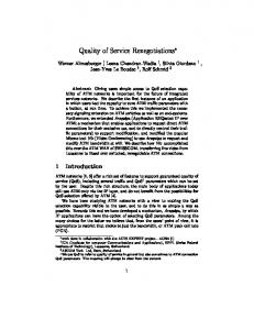
We consider message-passing distributed systems in which processes may fail by crashing, and messages may be delayed or dropped by communication links.1 In such systems, failure detectors typically provide a list of processes that are suspected to have crashed so far. A failure detector can be slow, i.e., it may take a long time to suspect a process that has crashed, and it can make mistakes, i.e., it may erroneously suspect some processes that are actually up (such a mistake is not necessarily permanent: the failure detector may later remove this process from its list of suspects). To be useful, a failure detector has to be reasonably fast and accurate. In this chapter, we propose a set of metrics for the QoS specification of failure detectors. In general, these QoS metrics should be able to describe the failure detector’s speed (how fast it detects crashes) and its accuracy (how well it avoids mistakes). Note that speed is with respect to processes that crash, while accuracy is with respect to processes that do not crash. A failure detector’s speed is easy to measure: this is simply the time that elapses from the moment when a process p crashes to the time when the failure detector starts suspecting p permanently. This QoS metric, called detection time, is illustrated in Fig. 2.1. How do we measure a failure detector’s accuracy? It turns out that determining a good set of accuracy metrics is a delicate task. To illustrate some of the subtleties involved, consider a system of two processes p and q connected by a lossy communication link, and suppose that the failure detector at q monitors process p. The 1 We assume that process crashes are permanent, or, equivalently, that a process that recovers from a crash assumes a new identity.
14
up
p
down trust
trust
FD at q
suspect
suspect TD
Figure 2.1: Detection time TD output of the failure detector at q is either “I suspect that p has crashed” or “I trust that p is up”, and it may alternate between these two outputs from time to time. For the purpose of measuring the accuracy of the failure detector at q, suppose that p does not crash. Consider an application that queries q’s failure detector at random times. For such an application, a natural measure of accuracy is the probability that, when queried at a random time, the output of the failure detector at q is “I trust that p is up” — which is correct. This QoS metric is the query accuracy probability. For example, in Fig. 2.2, the query accuracy probability of FD 1 at q is 12/(12 + 4) = .75. up
p
FD 1
12
FD 2 3
3 1
12
3 ... 1
4
12
4
4
1 ...
Figure 2.2: FD 1 and FD 2 have the same query accuracy probability of .75, but the mistake rate of FD 2 is four times that of FD 1.
The query accuracy probability, however, is not sufficient to fully describe the
15
up
p
FD 1
12
12
12
4 FD 2
8
4 8
8
4 8
8
8
Figure 2.3: FD 1 and FD 2 have the same mistake rate 1/16, but the query accuracy probabilities of FD 1 and FD 2 are .75 and .50, respectively.
accuracy of a failure detector. To see this, we show in Fig. 2.2 two failure detectors FD 1 and FD 2 such that (a) they have the same query accuracy probability, but (b) FD 2 makes mistakes more frequently than FD 1 .2 In some applications, every mistake causes a costly interrupt, and for such applications the mistake rate is an important accuracy metric. Note, however, that the mistake rate alone is not sufficient to characterize accuracy: as shown in Fig. 2.3, two failure detectors can have the same mistake rate, but different query accuracy probabilities. Even when used together, the above two accuracy metrics are still not sufficient. In fact, it is easy to find two failure detectors FD 1 and FD 2 , such that (a) FD 1 is better than FD 2 in both measures (i.e., it has a higher query accuracy probability and a lower mistake rate), but (b) FD 2 is better than FD 1 in another respect: specifically, whenever FD 2 makes a mistake, it corrects this mistake faster than FD 1; in other words, the mistake durations in FD 2 are smaller than in FD 1 . Having small mistake durations may be important to some applications. 2
The failure detector at q makes a mistake every time its output changes from “trust” to “suspect” while p is actually up.
16
As it can be seen from the above, there are several different aspects of accuracy that may be important to applications, and each aspect has a corresponding accuracy metric. In this chapter, we first identify six accuracy metrics (since the behavior of a failure detector is probabilistic, most of these metrics are random variables). We then use the theory of stochastic processes to determine their precise relation. This analysis allows us to select two accuracy metrics as the primary ones in the sense that: (a) they are not redundant (one cannot be derived from the other), and (b) together, they can be used to derive the other four accuracy metrics. In summary, we show that the QoS specification of failure detectors can be given in terms of three basic metrics, namely, the detection time and the two primary accuracy metrics that we identified. Taken together, these metrics can be used to characterize and compare the QoS of failure detectors.
2.1.2
Related Work
There is not much previous work on the QoS specification of failure detectors. In [CT96], unreliable failure detectors were introduced as an abstraction that can be used to solve some fundamental problems of fault-tolerant distributed computing, such as consensus, in asynchronous systems. This approach was later used and/or generalized in other works, e.g., [GLS95, DFKM96, FC96, ACT, ACT00, ACT99]. In all of these works, the failure detector specifications are defined in terms of the eventual behaviors of failure detectors (e.g., a process that crashes is eventually suspected). The eventual behavior, however, does not describe the QoS of failure detectors (e.g., how fast a process that crashes becomes suspected).
17
In [GM98], Gouda and McGuire measure the performance of some failure detector protocols under the assumption that the protocol stops as soon as some process is suspected to have crashed (even if this suspicion is a mistake). This class of failure detectors is less general than the one that we studied here: in our work, a failure detector can alternate between suspicion and trust many times. In [vRMH98], van Renesse et. al. propose a gossip-style randomized failure detector protocol. They measure the accuracy of this protocol in terms of the probability of premature timeouts.3 The probability of premature timeouts, however, is not an appropriate metric for the specification of failure detectors in general: it is implementation-specific and it cannot be used to compare failure detectors that use timeouts in different ways. This point is further explained in Section 2.4. In [VR00], Ver´ıssimo and Raynal study timing failure detectors, which detect timing failures (such as the delay of a message or the execution time of a task being longer than a given time bound). The class of timing failure detectors is more general than the class of failure detectors that detect crash failures. They also study QoS, but their work differs significantly from ours in that: What they study is QoS-FD — failure detectors that detect quality-of-service failures. More precisely, they study failure detectors that output some index (and other derived information) to indicate the quality of service of some system services (e.g. network connectivity). What we study here is the quality of service of (crash) failure detectors, i.e. how good a failure detector is in terms of detecting process crashes, and how to configure the failure detector to satisfy QoS requirements given by an application. 3
This is called “the probability of mistakes” in [vRMH98].
18
The rest of the chapter is organized as follows. In Section 2.2, we propose a set of QoS metrics for failure detectors. We quantify the relation between these metrics in Section 2.3, and conclude the chapter with a brief discussion in Section 2.4. In this chapter, we keep our presentation at an intuitive level. The formal definitions of our model and of our QoS metrics are developed using the theory of stochastic processes, and are given in Chapter 3.
2.2
Failure Detector Specification
We consider a system of two processes p and q. We assume that the failure detector at q monitors p, and that q does not crash. Henceforth, real time is continuous and ranges from 0 to ∞.
2.2.1
The Failure Detector Model
The output of the failure detector at q at time t is either S or T , which means that q suspects or trusts p at time t, respectively. A transition occurs when the output of the failure detector at q changes: An S-transition occurs when the output at q changes from T to S; a T-transition occurs when the output at q changes from S to T . We assume that there are only a finite number of transitions during any finite time interval. A failure detector history describes the output of the failure detector in an entire run. A failure pattern of process p is just a number F ∈ [0, ∞], denoting the time t at which p crashes; F = ∞ means that p does not crash. A run in which p does not crash is called a failure-free run. For each failure pattern, there is a corresponding
19
set of possible failure detector histories (as in [CT96]), and this set has a probability distribution. To understand this, consider the following example. Let F be the failure pattern in which p crashes at time 5. The failure detector at q may “detect” this crash at time 6, or 6.74, or 9, etc. This is the set H of failure detector histories corresponding to the failure pattern F . In a probabilistic system, some of the failure detector histories in H are more likely than others, and this is given by the probability distribution on H. With this probability distribution, quantities like “the probability that the crash of p is detected before time 8”, or “the expected detection time” are now meaningful. We consider only failure detectors whose behavior eventually reaches steady state, as we now explain.4 When a failure detector starts running, and for a while after, its behavior depends on the initial condition (such as whether initially q suspects p or not) and on how long it has been running. Typically, as time passes the effect of the initial condition gradually diminishes and its behavior no longer depends on how long it has been running — i.e., eventually the failure detector behavior reaches equilibrium, or steady state. In steady state, the probability law governing the behavior of the failure detector does not change over time. The QoS metrics that we propose refer to the behavior of a failure detector after it reaches steady state.
2.2.2
Primary Metrics
We propose three primary metrics for the QoS specification of failure detectors. The first one measures the speed of a failure detector. It is defined with respect to the 4
We omit the formal definition of steady state here; this definition is based on the theory of stochastic processes.
20
up
p
trust FD at q
suspect TM
suspect TG TMR
Figure 2.4: Mistake duration TM , Good period duration TG , and Mistake recurrence time TMR
runs in which p crashes. Detection time (TD ): Informally, TD is the time that elapses from p’s crash to the time when q starts suspecting p permanently. More precisely, TD is a random variable representing the time that elapses from the time that p crashes to the time when the final S-transition (of the failure detector at q) occurs and there are no transitions afterwards (Fig. 2.1). If there is no such final S-transition, then TD = ∞; if such an S-transition occurs before p crashes, then TD = 0. The next two metrics can be used to specify the accuracy of a failure detector. They are defined with respect to failure-free runs.5 Mistake recurrence time (TMR ): this measures the time between two consecutive mistakes. More precisely, TMR is a random variable representing the time that elapses from an S-transition to the next one (Fig. 2.4). If no new S-transition occurs, then TMR = ∞. Mistake duration (TM ): this measures the time it takes the failure detector to correct a mistake. More precisely, TM is a random variable representing the time that elapses from an S-transition to the next T-transition (Fig. 2.4). If no S-transition 5
In Section 2.4, we explain why these metrics also measure the failure detector accuracy in runs in which p crashes.
21
occurs, then TM = 0; if no T-transition occurs after an S-transition, then TM = ∞. As we discussed in the introduction, there are many aspects of failure detector accuracy that may be important to applications. Thus, in addition to TMR and TM , we propose four other accuracy metrics in the next section. We selected TMR and TM as the primary metrics because given these two, one can compute the other four (this will be shown in Section 2.3).
2.2.3
Derived Metrics
We propose the following four additional accuracy metrics (they are defined with respect to failure-free runs). Average mistake rate (λM ): this measures the rate at which a failure detector make mistakes, i.e., it is the average number of S-transitions per time unit. This metric is important to long-lived applications such as group membership and cluster management, where each mistake (each S-transition) results in a costly interrupt. Query accuracy probability (PA ): this is the probability that the failure detector’s output is correct at a random time. This metric is important to applications that interact with the failure detector by querying it at random times. Many applications are slowed down by failure detector mistakes. Such applications prefer a failure detector with long good periods — periods in which the failure detector makes no mistakes. This observation leads to the following two metrics. Good period duration (TG ): this measures the length of a good period. More precisely, TG is a random variable representing the time that elapses from a Ttransition to the next S-transition (Fig. 2.4). If no T-transition occurs, then TG = 0; if no S-transition occurs after a T-transition, then TG = ∞.
22
For short-lived applications, however, a closely related metric may be more relevant. Suppose that an application is started at a random time, and that this happens to occur somewhere inside a good period. In this case, we are interested in measuring the remaining portion of this good period: if it is long enough, the short-lived application will be able to complete its task within this period. The corresponding metric is as follows. Forward good period duration (TFG ): this is a random variable representing the time that elapses from a random time at which q trusts p, to the time of the next S-transition. If no such S-transition occurs, then TFG = ∞. If the probability that q trusts p at a random time is 0 (i.e. PA = 0), then TFG is always 0. At first sight, it may seem that, on the average, TFG is just half of TG (the length of a good period). But this is incorrect, and in Section 2.3 we give the actual relation between TFG and TG . We now give a simple example to illustrate how these definitions work. Example 1. Consider the following simple failure detector algorithm A: process p sends a heartbeat message to q every one time unit; process q suspects p initially; every time q receives a heartbeat message from p, q trusts p for one time unit, and by the end of the unit if q has not received any new heartbeat message, then q starts suspecting p. Suppose that algorithm A runs in the following simplified network environment: every heartbeat message is either lost, or is delivered instantaneously; each heartbeat message has an independent probability pL ∈ (0, 1) to be lost. We now analyze all seven metrics of this failure detector. In this system, if p does not crash, then q keeps trusting p if and only if the heartbeat messages are not lost.
23
Once a message is lost, q starts suspecting p immediately and the suspicion is kept until a new heartbeat message is received. For the detection time TD , let T be the time elapsed between the time t when p sends the last message and the time t′ when p crashes. T has a uniform distribution between 0 and 1. If the last heartbeat message is lost, then q starts suspecting p permanently at time t before p crashes, and so TD = 0 in this case. If the last message is not lost, then q starts suspecting p permanently at time t + 1, and so TD = 1− T in this case. Therefore, the distribution of TD is such that with probability pL , TD = 0, and with probability 1 − pL , TD = 1 − T , where T has a uniform distribution between 0 and 1. Thus we have
Pr (TD ≤ x) =
0
x y)dy,
E(TGk+1 ) . (k + 1)E(TG )
(2.3)
(2.4)
In particular, !
E(TG2 ) V(TG ) E(TG ) E(TFG ) = 1+ = . 2E(TG ) 2 E(TG )2
(2.5)
The fact that TG = TMR − TM holds is immediate by definition. Equalities (2.1) and (2.2) are intuitive, but (2.3), (2.4) and (2.5), which describe the relation between TG and TFG , are more complex. Moreover, (2.5) is counter-intuitive: one may think that E(TFG ) = E(TG )/2, but (2.5) says that E(TFG ) is in general larger than E(TG )/2 (this is a version of the “waiting time paradox” in the theory of stochastic processes [All90]). We now explain how Theorem 2.1 guided our selection of the primary accuracy metrics. Equalities (2.1), (2.2) and (2.3) show that λM , PA and TFG can be derived from TMR , TM and TG . This suggests that the primary metrics should be selected among TMR , TM and TG . Moreover, since TG = TMR − TM , it is clear that given the joint distribution of any two of them, one can derive the remaining one. Thus, two of TMR , TM and TG should be selected as the primary metrics, but which two? By choosing TMR and TM as our primary metrics, we get the following convenient property that helps to compare failure detectors: if FD 1 is better than FD 2 in terms of both E(TMR ) and E(TM ) (the expected values of the primary metrics) then we can be sure that FD 1 is also better than FD 2 in terms of E(TG ) (the expected values of
27
the other metric). We would not get this useful property if TG were selected as one of the primary metrics.6 We now demonstrate parts (2) and (3) of Theorem 2.1 with the example in the previous section. Example 2. Consider again the algorithm in Example 1. Since message losses are independent, the behavior of the failure detector does not depend on what happened in the past history, and so the distribution of failure detector histories in failure-free runs is ergodic. TG has a geometric distribution with parameter pL , so we have E(TG ) = 1/pL and V(TG ) = (1 − pL )/p2L . Similarly, we have E(TM ) = 1/(1 − pL ), and E(TMR ) = 1/pL + 1/(1 − pL ) = 1/[pL (1 − pL )]. With pL ∈ (0, 1), we have 0 < E(TMR ) < ∞ and E(TG ) 6= 0. Thus the conditions for Equalities (2.1)–(2.5) to hold are true. From Example 1, we know that λM = pL (1 − pL ) and PA = 1 − pL . Since E(TMR ) = 1/[pL (1 − pL )] and E(TG ) = 1/pL , Equalities (2.1) and (2.2) hold for this failure detector. We now check Equality (2.3). Given any x ∈ [0, ∞), let n = ⌊x⌋ and r = x − n. From Example 1, we know that TFG has the distribution such that with probability (1 − pL )i pL , TFG = T ′ + i, i ≥ 0, where T ′ has a uniform distribution from 0 to 1. Then Pr (TFG ≤ x) = Pr (TFG < n) + Pr (n ≤ TFG ≤ x) =
n−1 X i=0
(1 − pL )i pL + (1 − pL )n pL Pr (0 ≤ T ′ ≤ r)
= 1 − (1 − pL )n + rpL (1 − pL )n . 6
For example, FD 1 may be better than FD 2 in terms of both E(TG ) and E(TM ), but worse than FD 2 in terms of E(TMR ).
28
On the other side, for any y ∈ [i − 1, i), Pr (TG > y) = pL )j−1 pL = (1 − pL )i−1 . Thus 1 E(TG )
Z
x
0
Pr (TG > y) dy = pL = pL
" n Z X
j=i
i
i=1 i−1 " n X i=1
P∞
Pr (TG > y) dy +
(1 − pL )
i−1
Pr (TG = j) =
Z
j=i (1
n+r
n
+ r(1 − pL )
P∞
n
Pr (TG > y) dy #
−
#
= 1 − (1 − pL )n + rpL (1 − pL )n . Therefore, Equality (2.3) holds for this failure detector. Equalities (2.4) and (2.5) are direct consequences of Equality (2.3), and we only check Equality (2.5) here. From the distribution of TFG , we have E(TFG ) = P∞
i=0
E(T ′ + i)(1 − pL )i pL =
side,
P∞
i=0 (i + 1/2)(1 − pL )
E(TG ) V(TG ) 1+ 2 E(TG )2
!
1 = 2pL
i
pL = (2 − pL )/(2pL ). On the other
(1 − pL )/p2L 1+ 1/p2L
!
=
2 − pL . 2pL
Therefore, Equality (2.5) holds for this failure detector. Note that for this failure detector E(TFG ) = (2 − pL )/(2pL ) while E(TG ) = 1/pL , so E(TFG ) > E(TG )/2.
2.4
2
Discussion
On the Probability of Premature Timeouts For timeout-based failure detectors, the probability of premature timeouts is sometimes used as the accuracy measure: this is the probability that when the timer is set, it will prematurely timeout on a process that is actually up. The problem with this measure, however, is that (a) it is implementation-specific, and (b) it is not
29
useful to applications unless it is given together with other implementation-specific measures, e.g., how often timers are started, whether the timers are started at regular or variable intervals, whether the timeout periods are fixed or variable, etc. (many such variations exist in practice [Bra89, GM98, vRMH98]). Thus, the probability of premature timeouts is not a good metric for the specification of failure detectors, e.g., it cannot be used to compare the QoS of failure detectors that use timeouts in different ways. The six accuracy metrics that we identified in this paper do not refer to implementation-specific features, in particular, they do not refer to timeouts at all.
Accuracy Metrics and Runs with Crashes To measure the accuracy of a failure detector that monitors a process p, we considered runs in which p does not crash. In real systems, however, such runs rarely occur: p is likely to crash eventually. Are our accuracy metrics applicable to such systems? The answer is yes, as we now explain. Note that the output of any failure detector implementation at a time t should not depend on what happens after time t, i.e., the implementation does not predict the future.7 Therefore, the steady state behavior of a failure detector before a process p crashes is the same as its steady state behavior in runs in which p does not crash. Thus, our accuracy metrics also measure the accuracy of a failure detector in runs in which p eventually crashes (provided that this crash occurs after the failure detector has reached its steady state behavior). 7
Our model can enforce this assumption by imposing some restriction on the sets of failure detector histories and their associated distributions (see Chapter 3).
30
Good Periods versus Stable Periods Recall that a good period of a failure detector is defined in terms of runs in which p does not crash. It starts when the failure detector trusts p (makes a T-transition) and terminates when the failure detector erroneously suspects p (makes an S-transition). In contrast, a stable period of a system starts when the failure detector trusts p and p is up, and terminates when either: (a) the failure detector suspects p, or (b) p crashes. The length of stable periods is an important measure for many applications. This measure, however, cannot be part of the QoS specification of failure detectors: since a failure detector has no control over process crashes, it cannot by itself ensure “long” stable periods, even if it is very accurate. To measure the length of a stable period in a system, one can use measures on the accuracy of the failure detector and on the likelihood of crashes. For example, let TG be the random variable representing the length of a good period of the failure detector, and C be the random variable representing the lifetime of process p. Assume that C has an exponential distribution (so that at any given time at which p is still up, the remaining lifetime of p has the same distribution as C). Let S be the random variable representing the length of a stable period after the failure detector has reached steady state. Then the distribution of S is given by Pr (S ≤ x) = 1 − Pr (C > x)Pr (TG > x). Intuitively, this is because a stable period terminates as soon as the failure detector makes a mistake or p crashes.
Chapter 3 Stochastic Modeling of Failure Detectors and Their Quality-of-Service Specifications 3.1
Introduction
In Chapter 2, we proposed a set of metrics for the QoS specification of failure detectors. The definitions of failure detectors and the QoS metrics were kept at an intuitive level to emphasize the main ideas of the QoS specification of failure detectors. In this chapter, we give a rigorous formalization of failure detectors and their QoS metrics based on stochastic modeling, in particular the theory of marked point processes (c.f. [Sig95]). Upon the first reading, readers can skip this chapter and read Chapter 4 without any difficulty. In the formalization, we first define random failure detector histories that model
31
32
the probabilistic behaviors of failure detectors. We show that a random failure detector history is an extension of a (particular type of) random marked point process. We next define failure detectors as mappings from failure patterns to random failure detector histories. This is an extension to the failure detector model of [CT96]. We then define some particular random failure detector histories as the steady state behaviors of a failure detector and use them to define the QoS metrics. Some of these random failure detector histories match with the stationary versions of random marked point processes. Finally, we analyze the relation between the QoS metrics we defined. The analysis is based on the results in the theory of marked point processes, such as Birkhoff’s Ergodic Theorem for marked point processes, and the empirical inversion formulas. The relations we present in this chapter are more general than the results in Theorem 2.1 of Chapter 2. The rest of the chapter is organized as follows. In Section 3.2, we define the failure detector model, which includes the definitions of random failure detector histories, failure detectors, and the steady state behaviors of failure detectors. In Section 3.3, we define the QoS metrics and analyze the relation between these metrics. In Appendix A, we summarize relevant definitions and results in the theory of marked point processes.
3.2
Failure Detector Model
As in Chapter 2, we consider a system of two processes p and q, and a failure detector at q that monitors p. We assume that q does not crash. Real time is continuous and ranges from 0 to ∞.
33
3.2.1
Failure Detector Definition
As described in Section 2.2.1, the output of the failure detector is denoted as either S or T , and it has two types of transitions: S-transitions and T-transitions. Roughly speaking, a failure detector history describes the output of the failure detector in an entire run, and it can be represented by the initial output and the times at which transitions occur. More precisely, we define a failure detector history as follows. Let R, R+ , and Z+ denote the set of real numbers, nonnegative real numbers, and nonnegative integers, def
respectively. Let K = {S, T }. For x ∈ K, let x denote the element other than x in K. A failure detector history is given as ψ = hk, {tn : n ∈ I}i such that (1) k ∈ K; (2) I = Z+ or I = {0, 1, . . . , m − 1} for some m ∈ Z+ (if m = 0, then I = ∅); (3) tn ∈ R+ for all n ∈ I; (4) if I = Z+ , then 0 ≤ t0 < t1 < t2 < · · ·, and limn→∞ tn = ∞; (5) if |I| = m < ∞, then 0 ≤ t0 < t1 < t2 < · · · < tm−1 . In the representation of failure detector history ψ, k represents the output of the failure detector at time 0, and the increasing sequence {tn } represents the times at which failure detector transitions occur. We call tn the n-th transition time (so ψ starts with the zeroth transition). When t0 > 0, ψ = hk, {tn }i represents a run in which the failure detector outputs k in the period [0, t0), makes a transition at time t0, then outputs k in the period [t0, t1 ), and then makes another transition at time t1, and so on. When t0 = 0, ψ = hk, {tn }i represents a run in which failure detector has a transition at time 0, then outputs k in the period [t0, t1), makes a transition at
34
time t1 , and then outputs k in the period [t1, t2), and so on. Allowing a transition at time 0 is to conform with the representation of marked point processes (as in [Sig95]), which is the basic tool we use to model the failure detectors. Intuitively it makes sense when there is output before time 0, and this can happen if the time line is shifted. The requirement limn→∞ tn = ∞ in (4) enforces that there are only a finite number of transitions in any bounded time interval. For a failure detector history ψ = hk, {tn : n ∈ I}i, we define the n-th interdef
transition time Tn of ψ as follows. If |I| = ∞, then Tn = tn+1 − tn for all n ≥ 0; def
def
if |I| = m < ∞, then (a) if m = 0, then T0 = ∞ and Tn = 0 for n ≥ 1; and (b) if def
def
def
m ≥ 1, then Tn = tn+1 − tn for 0 ≤ n ≤ m − 2, Tm−1 = ∞, and Tn = 0 for n ≥ m. To model the probabilistic behavior of a failure detector, we need to define random failure detector histories with probability distributions over the set of failure detector histories. To do so, we first need to define what are the subsets of failure detector histories that we can assign probability to. Formally, we need to define a σ-field which contains all measurable subsets of failure detector histories. This is done as follows. def
∞ Let H be the set of all failure detector histories. Let Z∞ + = Z+ ∪{∞}. for m ∈ Z+ ,
let H(m) be the set of all failure detector histories with exactly m transitions, i.e. def
H(m) = {ψ = hk, {tn : n ∈ I}i : |I| = m}. Thus {H(m) : m ∈ Z∞ + } forms a partition of H. We next define the Borel σ-field B(H(m)) of H(m) for each m ∈ Z∞ +. When m < ∞, H(m) is a subset of K × Rm , where Rm is the m-dimensional Euclidean space with the Borel σ-field B(Rm). Let B(K × Rm ) be the product σ-field generated by {K × B : K ⊆ K, B ∈ B(Rm )}. It is easy to check that def
H(m) ∈ B(K × Rm ). Then, we get the Borel σ-field B(H(m)) = {E : E ∈ B(K ×
35
Rm ), E ⊆ H(m) }. When m = ∞, H(∞) is a subset of K × RZ+ , where RZ+ is the set of all countably infinite sequences of real numbers. It is known (see e.g. [Sig95]) that RZ+ is a complete separable metric space, and the Borel σ-field B(RZ+ ) is well defined. Let B(K × RZ+ ) be the product σ-field generated by {K × B : K ⊆ K, B ∈ B(RZ+ )}. It is easy to check that H(∞) ∈ B(K × RZ+ ). Then, we get the Borel σ-field def
B(H(∞)) = {E : E ∈ B(K × RZ+ ), E ⊆ H(∞)}. With the above definitions of B(H(m)) for all m ∈ Z∞ + , we then define the Borel σ-field B(H) of H to be {
S
m∈Z∞ +
Em : Em ∈ B(H(m))}. Hence we have a measurable
space (H, B(H)) on the set of all failure detector histories. Some simple examples of Borel sets in H are: (1) {ψ ∈ H : k = S}, the set of failure detector histories in which the output at time 0 is S; (2) {ψ ∈ H : t0 ≤ x}, the set of failure detector histories in which the zeroth transition occurs within x time units; and (3) {ψ ∈ H : T0 ≤ x}, the set of failure detector histories in which the zeroth intertransition time is at most x time units. It is easy to verify that B(H) can also be generated from the following collection of the sets: {ψ = hk, {tn : n ∈ I}i ∈ H : |I| = m, k ∈ K, tn0 ≤ x0, . . . , tnl ≤ xl },
(3.1)
where m ∈ Z∞ + , K ⊆ K, l ∈ I, 0 ≤ n0 < · · · < nl < m, xi ∈ R+ . We define a random failure detector history to be a measurable mapping Ψ : Ω → H, with (Ω, F , P ) as the underlying probability space. With this definition, the randef
dom failure detector history Ψ has the probability distribution P (Ψ ∈ E) = P ({ω ∈ Ω : Ψ(ω) ∈ E}) defined for all E ∈ B(H). For convenience, we use {Ψ ∈ E} as a
36
short hand for {ω ∈ Ω : Ψ(ω) ∈ E}. Let Ψ be the set of all random failure detector histories. A failure pattern F of process p is just a number F ∈ [0, ∞], denoting the time F at which p crashes; F = ∞ means that p does not crash, and we call this pattern failure-free pattern. Let F denote the set of all failure patterns. Thus F = [0, ∞]. A failure detector D is a mapping D : F → Ψ. Intuitively, the random failure detector history D(F ) characterizes the probabilistic behavior of the failure detector output when process p crashes at time F . This is an extension of the failure detector definition in [CT96] to model the probabilistic behavior of the failure detector output.
3.2.2
Failure Detector Histories as Marked Point Processes
We now build the relation between failure detector histories and marked point processes. Given a failure detector history ψ = hk, {tn : n ∈ I}i where I 6= ∅, let kn be the output of the failure detector at time tn for all n ∈ I. Thus, we know that the transition occurred at time tn is a kn -transition, and in period [tn, tn+1 ), the failure detector output is kn . The relation between k and kn ’s is: (1) if t0 = 0, then k0 = k2 = · · · = k and k1 = k3 = · · · = k; and (2) if t0 > 0, then k0 = k2 = · · · = k def
def
and k1 = k3 = · · · = k. For notational convenience, let t−1 = 0, and k−1 = k. With kn ’s, the failure detector history ψ can be equivalently represented as ψ = {(tn , kn ) : n ∈ I}. When I = Z+ , this representation coincides with the representation of a simple marked point process as given in [Sig95]. In fact, A failure detector history with an infinite number of transitions can be directly modeled as a simple marked point process, with transitions as events and K as the mark space.
37
Therefore, definitions and results for marked point processes can be directly applied to failure detector histories with an infinite number of transitions. For consistency and convenience, we extend some of the definitions to include failure detector histories with only a finite number of transitions. One important extension is the shift mappings on failure detector histories with a finite number of transitions, as given below. Suppose θs : H → H is a shift mapping defined on all failure detector histories. Intuitively, for a failure detector history ψ, θs ψ is the failure detector history obtained from ψ by shifting the origin to s, using the output at time s as the initial output, re-labeling transitions at and after s as t0, t1 , . . ., and ignoring the portion of the failure detector history before s. More precisely, if s = 0, then θs is the identity mapping; if ψ has an infinite number of transitions, then ψ is also a simple marked point process, and thus θs ψ is defined as in Appendix A. Now suppose s > 0 and ψ = hk, {tn : n ∈ I}i has only a finite number of transitions, i.e., |I| = m < ∞. If ti−1 < s ≤ ti for some i ∈ I, then def
θs ψ = hk ′ , {ti+n − s : 0 ≤ n ≤ m − 1 − i}i, where k ′ is the output at time s, and def
k ′ = ki if s = ti ; k ′ = ki if s < ti . If s > tm−1 , then θs ψ = hkm−1 , ∅i. We now define shift mapping by event time θ(j) for j ≥ 0. Intuitively, for a failure detector history ψ, θ(j) ψ is a failure detector history obtained from ψ by shifting the origin to the time of j-th transition in ψ, and if ψ does not have enough transitions, then the origin is shifted to the last transition of ψ. More precisely, if ψ has at def
least j + 1 transitions, then θ(j) ψ = θtj ; if ψ has less than j + 1 transitions, then def
θ(j)ψ = θtm−1 , where m is the number of transitions in ψ. We then let def
ψs = θs ψ
and
def
ψ(j) = θ(j) ψ.
(3.2)
38
Note that ψ(j) always has a transition at the origin, except the case when ψ itself has no transition at all. For a random failure detector history Ψ : Ω → H, let Ψs : Ω → H be a random failure detector history obtained from Ψ by shifting the origin to time s, that is, Ψs (ω) = Ψ(ω)s for all ω ∈ Ω. Similarly, let Ψ(j) : Ω → H be a random failure detector history obtained from Ψ by shifting the origin to the time of the j-th transition, that is, Ψ(j)(ω) = Ψ(ω)(j) for all ω ∈ Ω. Intuitively,Ψs represents what you see if you always start observing Ψ at time s, and Ψ(j) represents what you see if you always start observing Ψ at the j-th transition. Shift mapping is an important tool to the study of the steady state behaviors of failure detectors, as we discuss in the next section.
3.2.3
The Steady State Behaviors of Failure Detectors
We consider failure detectors whose behaviors eventually reach the steady state. Roughly speaking, when a failure detector starts running, and for a while after, its behavior depends on the initial condition (such as whether initially q suspects p or not) and on how long it has been running. Typically, as time passes the effect of the initial condition gradually diminishes and its behavior no longer depends on how long it has been running — i.e., eventually the failure detector behavior reaches equilibrium, or steady state. Suppose that while p is still up, the behavior of the failure detector reaches a steady state. We consider two kinds of behaviors in this case: First, if p remains up, what would be the behavior of the failure detector? Second, if p crashes, what would be the behavior of the failure detector in response of the crash of p?
39
We now formally define several random failure detector histories that capture such steady state behaviors. Let D be the failure detector in consideration. The Steady State Behavior If p Does Not Crash def
Let F = ∞ be the failure-free pattern of p. Then Ψ = D(F ) defines the behavior of the failure detector output under this failure-free pattern. Suppose the underlying probability space defining Ψ is (Ω, F , P ). The steady state behavior of Ψ is given by its event stationary version Ψ0 and time stationary version Ψ∗ , if they exist. Formally, they are defined by the following distributions (assuming they exist), just as the definitions in Section 2.3 of [Sig95]:1
def
X 1 n−1 P (Ψ(j) ∈ E), for all E ∈ B(H), n→∞ n j=0
(3.3)
1 t→∞ t
(3.4)
Pr (Ψ0 ∈ E) = lim def
Pr (Ψ∗ ∈ E) = lim
Z
0
t
P (Ψs ∈ E) ds, for all E ∈ B(H).
The event stationary version Ψ0 is obtained by averaging the distribution of Ψ(j) over all transition times, and the time stationary version Ψ∗ is obtained by averaging the distribution of Ψs over all times. Such average distributions are referred to as empirical distributions in [Sig95]. The intuitive meanings of (3.3) and (3.4) are: if we randomly pick a transition and start observing Ψ after this transition, the random failure detector history we observed is given by the event stationary version Ψ0 ; if we randomly pick a real time s and then observe the behavior of Ψ after s, then the 1
Note that in (3.3) and (3.4) we use the notation Pr (·) to avoid the complication of specifying the underlying probability spaces for Ψ0 and Ψ∗ . These stationary versions can be defined in probability spaces different from Ψ, but there is no need to specify them here since we are only interested in the probability distributions of Ψ0 and Ψ∗ . We will use the notation Pr (·) whenever it is convenient for us.
40
random failure detector history we observed is given by the time stationary version Ψ∗ . Using the expressions in [Sig95], Ψ0 is the version of Ψ when we randomly observe Ψ way out at a transition, and Ψ∗ is the version of Ψ when we randomly observe Ψ way out in time. Intuitively, Ψ0 is event stationary, i.e., the distribution does not change if Ψ0 is shifted by transition times (see Appendix A for its definition), because after already randomly observing Ψ way out at a transition to obtain Ψ0, observing Ψ several transitions later makes no difference to the distribution of Ψ0. Similarly, Ψ∗ is time stationary, i.e, the distribution does not change if Ψ∗ is shifted by time, because after already randomly observing Ψ way out in time to obtain Ψ∗ , observing Ψ some time units later makes no difference to the distribution of Ψ∗ . Lemma 3.1 Ψ0 is event stationary and Ψ∗ is time stationary. Proof. The proof is the same as the proof in [Sig95] p.26, except that the definitions of shift mappings are extended to include the case where the number of transitions
2
are finite.
We say that the behavior of the failure detector D reaches steady state in failurefree runs if the distributions defined in (3.3) and (3.4) exist. The accuracy metrics of the failure detector are defined with respect to the steady state behavior of the failure detector in failure-free runs, i.e., with respect to stationary versions Ψ0 and Ψ∗ . To further understand the stationary versions Ψ0 and Ψ∗ , we break down events in B(H) into different categories and study them separately. From Section 3.2.1, we know that {H(m) : m ∈ Z∞ + } is a partition of H, and B(H) = { Em ∈ B(H(m))}. Therefore, for any event E =
S
m∈Z∞ +
S
m∈Z∞ +
Em :
Em , if we know Pr (Ψ0 ∈ Em )
41
for all m ∈ Z∞ + , then by the additivity of the probability measure we know that Pr (Ψ0 ∈ E) =
P
m∈Z∞ +
Pr (Ψ0 ∈ Em ). The case for Pr(Ψ∗ ∈ E) is similar. Thus, we
now focus on Pr (Ψ0 ∈ E) and Pr (Ψ∗ ∈ E) with E ∈ B(H(m)), for each m ∈ Z∞ +. Let ES and ET be the sets of all failure detector histories in which eventually the output is always S or T , respectively. Thus ES ∪ ET contains all failure detector def
def
Ψ histories with a finite number of transitions. Let pΨ S = P (Ψ ∈ ES ) and pT = P (Ψ ∈ Ψ ET ). Thus pΨ S and pT are the probabilities that eventually the output of the random def
failure detector history Ψ is always S or always T , respectively. Let pΨ ∞ = P (Ψ ∈ H(∞) ), the probability that Ψ has an infinite number of transitions. Ψ Ψ Proposition 3.2 pΨ S + pT + p∞ = 1.
Proof. It is direct from the fact that ES , ET , and H(∞) are disjoint and ES ∪ ET ∪ H(∞) = H.
2
Ψ Probabilities pΨ S and pT are used to characterize the steady state behavior of
failure detector histories with only a finite number of transitions. Intuitively, if a run of the failure detector only has a finite number of transitions, then in steady state the failure detector should keep its final output value. In other words, when you randomly observe a failure detector history with a finite number of transitions way out in time or way out at a transition, with probability one what you observe is the portion in which the failure detector keeps its final output value. The probability Ψ that the output you observe is S or T is given by pΨ S or pT , respectively. This is
formalized in the following lemma. Lemma 3.3 ∗ Ψ (1) Pr (Ψ∗ ∈ {hS, ∅i}) = pΨ S , and Pr (Ψ ∈ {hT, ∅i}) = pT ;
42
(2) For all m ∈ Z+ \ {0}, for all E ∈ B(H(m)), Pr (Ψ∗ ∈ E) = 0; 0 Ψ (3) Pr (Ψ0 ∈ {hS, ∅i, hS, {0}i}) = pΨ S , and Pr (Ψ ∈ {hT, ∅i, hT, {0}i}) = pT ;
(4) For all m ∈ Z+ \ {0}, for all E ∈ B(H(m)), if E does not contain hS, {0}i or hT, {0}i, then Pr (Ψ0 ∈ E) = 0. Proof. (1) Let E = {hS, ∅i}. We have that if s ≤ t, then {Ψs ∈ E} ⊆ {Ψt ∈ E}, i.e., if a failure detector history remains the output S from time s on, then it of course remains the output S from a later time t on. Thus P (Ψs ∈ E) ≤ P (Ψt ∈ E). It is clear that {Ψt ∈ E} ↑ {Ψ ∈ ES }, i.e., as t → ∞, {Ψt ∈ E} monotonically increasing and tends to {Ψ ∈ ES } from below. Then for integer valued n, {Ψn ∈ E} ↑ {Ψ ∈ ES }. Since the probability measure is continuous from below (see e.g. [Bil95], p.25), we have P (Ψn ∈ E) ↑ P (Ψ ∈ ES ), then it is also true that P (Ψt ∈ E) ↑ P (Ψ ∈ ES ). From (3.4), we have Z
1 t P (Ψs ∈ E) ds t→∞ t 0 Z 1 t ≤ lim P (Ψt ∈ E) ds = lim P (Ψt ∈ E) = P (Ψ ∈ ES ) = pΨ S. t→∞ t 0 t→∞
Pr (Ψ∗ ∈ E) = lim
On the other hand, from P (Ψt ∈ E) ↑ P (Ψ ∈ ES ), we have that for all ǫ > 0, there exists K such that for all s ≥ K, P (Ψs ∈ E) ≥ pΨ S − ǫ. Then 1 Pr (Ψ ∈ E) = lim t→∞ t ∗
Z
0
t
1 P (Ψs ∈ E) ds ≥ lim t→∞ t
Z
t
K
�
�
Ψ pΨ S − ǫ ds = pS − ǫ.
∗ Ψ Let ǫ → 0, we have Pr (Ψ∗ ∈ E) ≥ pΨ S . Therefore, Pr (Ψ ∈ E) = pS . Similarly, we
can prove that Pr(Ψ∗ ∈ {hT, ∅i}) = pΨ T. (2) For all E ∈ B(H(m)) with m ∈ Z+ \ {0}, since E ∩(H(∞) ∪{hS, ∅i, hT, ∅i}) = ∅, Ψ ∗ we have Pr (Ψ∗ ∈ E) ≤ 1−Pr (Ψ∗ ∈ H(∞) )−pΨ S −pT . Thus, to prove Pr (Ψ ∈ E) = 0, Ψ Ψ Ψ it is enough to show that Pr (Ψ∗ ∈ H(∞)) = pΨ ∞ , since we know that pS +pT +p∞ = 1.
43
(∞) To prove Pr (Ψ∗ ∈ H(∞)) = pΨ } = {Ψ ∈ H(∞) }, i.e., a ∞ , note that {Ψs ∈ H
failure detector history has an infinite number of transitions from time s on if and only if itself has an infinite number of transitions. Then we have ∗
Pr (Ψ ∈ H
(∞)
Z
1 t ) = lim P (Ψs ∈ H(∞)) ds t→∞ t 0 Z 1 t P (Ψ ∈ H(∞) ) ds = P (Ψ ∈ H(∞) ) = pΨ = lim ∞. t→∞ t 0
(3) and (4) have similar proofs as those of (1) and (2).
2
We now look at failure detector histories with an infinite number of transitions. We know that with probability pΨ ∞ , Ψ has an infinite number of transitions. If Ψ Ψ pΨ ∞ = 0, then pS + pT = 1, and in the stationary versions of Ψ, only trivial histories
that never change the failure detector outputs have a nonzero probability. (∞) We now consider the case when pΨ . ∞ > 0. In this case, we restrict Ψ onto H Ψ Ψ More precisely, we first define the restricted probability space (ΩΨ ∞ , F∞ , P∞ ) such that Ψ Ψ −1 (∞) Ψ = {B : B ∈ F , B ⊆ ΩΨ ), (2) F∞ (1) ΩΨ ∞ }, and (3) P∞ (B) = P (B)/p∞ ∞ = Ψ (H Ψ for all B ∈ F∞ . We then define the restricted random failure detector history Ψ∞ as (∞) the measurable mapping from ΩΨ such that Ψ∞ (ω) = Ψ(ω) for all ω ∈ ΩΨ ∞ to H ∞.
Since a failure detector history in H(∞) is also a simple marked point process, Ψ∞ is also a random marked point process as defined in [Sig95]. Ψ∞ , as a random marked point process, has its own event stationary version Ψ0∞ and time stationary version Ψ∗∞ (see definitions in Appendix A). The following lemma gives the relation between the distributions of Ψ0 , Ψ∗ and Ψ0∞ , Ψ∗∞ . (∞) 0 Lemma 3.4 If pΨ ), Pr (Ψ0 ∈ E) = pΨ ∞ > 0, then for all E ∈ B(H ∞ ∗ Pr (Ψ∞ ∈ E), ∗ and Pr (Ψ∗ ∈ E) = pΨ ∞ ∗ Pr (Ψ∞ ∈ E).
44
Proof. Direct from (3.3), (3.4), (A.5), (A.6) and the definition of the probability
2
Ψ measure P∞ .
The Steady State Behavior after p Crashes We now define a random failure detector history that represents the steady state behavior of the failure detector after p crashes. Formally, a post-crash version Ψc of failure detector D is a random failure detector history defined by the following distribution (assuming it exists): 1 Pr (Ψ ∈ E) = lim t→∞ t c
def
Z
0
t
Pr (D(s)s ∈ E) ds, for all E ∈ B(H).
(3.5)
Intuitively, (3.5) means that if we randomly pick a time s at which p crashes and then observe the behavior of the failure detector after time s, the random failure detector history we observed is given by the post-crash version Ψc . So, similarly to Ψ0 and Ψ∗ , we say that Ψc is the version of the failure detector D when we randomly observe D way out at a time when p crashes. Ψc is obtained by averaging the distribution of D(s)s , the post-crash behavior of the failure detector D, over all crash times. Thus it is also an empirical distribution. We say that the failure detector D has steady state behavior after p crashes if the distribution defined in (3.5) exists. One primary metric, the detection time, is defined with respect to the steady state behavior after p crashes, i.e., with respect to the post-crash version Ψc . Non-Futuristic Property Before p crashes, no failure detector implementation can tell whether p will crash later or not, i.e., the failure detector cannot predict the future. Therefore, the behavior
45
of the failure detector up to any time t at which p is still up should be the same as the behavior of the failure detector in the same period in failure-free runs. We now formalize this idea. (m)
For all m ∈ Z+ and for all t ∈ R+ , let H≤t be the subset of H(m) such that (m)
the time of the last transition of any failure detector history in H≤t is at most t, (m) def
(m)
i.e., H≤t = {ψ ∈ H(m) : tm−1 ≤ t}. So H≤t gives the set of failure detector history (m)
prefixes up to time t that contains exactly m transitions. Clearly H≤t ∈ B(H(m)), (m)
(m)
and so we can define the Borel σ-field B(H≤t ) = {E : E ∈ B(H(m)), E ⊆ H≤t }. Let H≤t =
S
(m)
m∈Z+
H≤t . H≤t contains all failure detector history prefixes up to time t.
The Borel σ-field of H≤t is defined as B(H≤t) = {
S
m∈Z+
(m)
Em : Em ∈ B(H≤t )}. We
define a prefix mapping f≤t : H → H≤t , such that for any failure detector history ψ ∈ H, f≤t (ψ) is the failure detector history prefix that only contains the transitions of ψ up to time t. It is easy to verify that f≤t is a measurable mapping. We now formally define the probabilistic behavior of a failure detector history up to some time t. Given a random failure detector history Ψ : Ω → H, the random failure detector history prefix up to time t is the measurable mapping Ψ≤t : Ω → H≤t such that Ψ≤t = f≤t ◦ Ψ. We say that a failure detector D is non-futuristic (or not predicting the future) if for all t ∈ R+ , for all t1, t2 ∈ R∞ + and t1 , t2 > t, D(t1 )≤t and D(t2 )≤t have the same distribution, i.e., for all E ∈ B(H≤t ), Pr (D(t1 )≤t ∈ E) = Pr (D(t2 )≤t ∈ E). Intuitively, this means that as long as p has not crashed yet by time t, the probabilistic behavior of the failure detector up to time t is the same no matter whether or when p may crash later. In other words, the failure detector does not provide hints on whether or when process p will crash in the future.
46
3.3
Failure Detector Specification Metrics
With the formal model of the failure detector given in the previous section, we are now ready to formally define the QoS metrics of the failure detector introduced in Chapter 2. def
Let D be a failure detector. Let R∞ + = R+ ∪ {∞}.
3.3.1
Definitions of Metrics
Detection time (TD ): TD is defined from the post-crash version Ψc of D. Suppose Ψc : Ωc → H, with (Ωc , F c , P c ) as the underlying probability space. We first define a measurable mapping fD : H → R∞ + such that for any failure detector history ψ ∈ H, fD (ψ) is: (a) 0, if ψ has no transition and the output is always S; or (b) the time of the last transition, if ψ has a finite number of transitions and the output after the last transition is always S; or (c) ∞ otherwise. Then TD : Ωc → R∞ + is the random variable such that TD = fD ◦ Ψc . That is, given any particular post-crash history ψ, TD = fD (ψ) is the time elapsed from the time of crash to the time when the failure detector starts suspecting p permanently, and the distribution of TD is determined by the distribution of Ψc , which is defined in (3.5). All accuracy metrics are defined with respect to the steady state behavior in failure-free runs, i.e., with respect to the stationary versions Ψ0 and Ψ∗ of the random def
failure detector history Ψ = D(∞). For the convenience of studying the relations between the accuracy metrics in the next section, we assume that Ψ, Ψ0 and Ψ∗ use the same underlying probability space (Ω, F , P ) (one can always construct some common space supporting all of them).
47
The following three accuracy metrics are defined in terms of the event stationary version Ψ0 . Recall from Section 3.2.1 that T0 and T1 are defined as the zeroth and the first intertransition time of a given failure detector history ψ. Thus T0 and T1 are actually measurable mappings from H to R∞ +. Mistake recurrence time (TMR ): We define a measurable mapping fMR : H → ∞ R∞ + such that fMR = T0 + T1 . Then TMR : Ω → R+ is the random variable such that
TMR = fMR ◦Ψ0 . Intuitively, TMR is the length of the first two consecutive periods, one trust period and one suspicion period, of Ψ0 . We call any two consecutive periods a recurrence interval. Since Ψ0 is event stationary, the distribution of the length of any recurrence interval is the same, and thus we only take the first recurrence interval of Ψ0 . TMR represents the length of the recurrence interval when we randomly observe the failure detector output way out at a transition in some failure-free run, and its distribution is determined by the distribution of Ψ0, which is defined in (3.3). Note that when defining TMR we do not restrict the recurrence interval to be started and ended with S-transitions. This is because in steady state whether you observe at an S-transition or a T-transition does not change the distribution of the length of the recurrence interval, and so we choose not to make this restriction for convenience. Mistake duration (TM ): we define a measurable mapping fM : H → R∞ + such that for any failure detector history ψ = hk, {tn }i ∈ H, fM (ψ) = T0 (ψ) if k = S, and fM (ψ) = T1 (ψ) if k = T . Then TM : Ω → R∞ + is the random variable such that TM = fM ◦ Ψ0 . Recall that after being shifted by a transition time, any failure detector history has a transition at origin (i.e., t0 = 0) except the histories with no transitions at all. Thus the definition of fM guarantees that it always takes the length of the first suspicion (mistake) period from the event stationary version Ψ0.
48
Therefore, TM represents the length of the mistake period when we randomly observe the failure detector output way out at an S-transition in some failure-free run, and its distribution is determined by the distribution of Ψ0. Good period duration (TG ): The definition of TG is symmetric to that of TM . we define a measurable mapping fG : H → R∞ + such that for any failure detector history ψ = hk, {tn }i ∈ H, fG (ψ) = T0(ψ) if k = T , and fG (ψ) = T1(ψ) if k = S. 0 Then TG : Ω → R∞ + is the random variable such that TG = fG ◦ Ψ . Intuitively,
TG represents the length of the trust (good) period when we randomly observe the failure detector output way out at a T-transition in some failure-free run, and its distribution is determined by the distribution of Ψ0. The following three accuracy metrics are defined in terms of the time stationary version Ψ∗. Query accuracy probability (PA ): Let BT be the set of failure detector histodef
ries with output T at time 0. Then PA = P (Ψ∗ ∈ BT ). Intuitively, when we randomly observe the failure detector output way out at a time t in some failure-free run, the probability that the output at time t is T is just the probability that the output is T at time 0 of the time stationary version Ψ∗ . Therefore, PA is the probability that, when queried at a random time in some failure-free run, the output of the failure detector is T (and thus is correct). Average mistake rate (λM ): We define a measurable mapping NS : H → R+ such that for any failure detector history ψ, NS (ψ) is the number of S-transitions in the period (0, 1]. Thus NS ◦ Ψ∗ is a random variable representing the number of S-transitions of Ψ∗ in the unit interval (0, 1]. Since Ψ∗ is time stationary, NS ◦ Ψ∗ is the number of S-transitions in any unit interval when we randomly observe the
49
failure detector output way out in time in some failure-free run. Then λM is defined as E(NS ◦ Ψ∗ ), the expected value of NS ◦ Ψ∗ . Forward good period duration (TFG ): Roughly speaking, we define TFG as the time from the origin to the first transition of Ψ∗ , conditioned on the fact that the output of Ψ∗ at the origin is T . Since Ψ∗ is obtained when we randomly observe the failure detector output way out in time in failure-free runs, TFG represents the time elapsed from a random time at which q trusts p to the time of the next S-transition. We now formally define TFG . If PA = 0, then let TFG ≡ 0, i.e., if the probability that q trusts p at a random time is 0, then TFG is always 0. If PA > 0, then we define a random failure detector history Ψ∗T obtained by restricting Ψ∗ onto BT . More precisely, we first define a restricted probability space (ΩT , FT , PT ) such that (1) ΩT = {Ψ∗ ∈ BT }, (2) FT = {B : B ∈ F , B ⊆ ΩT }, and (3) PT (B) = P (B)/PA for all B ∈ FT . Then Ψ∗T : ΩT → BT is the random failure detector history such that Ψ∗T (ω) = Ψ∗ (ω) for all ω ∈ ΩT . Intuitively, Ψ∗T is the version of Ψ∗ conditioned on the fact that the output at the origin is T . Let fFG : BT → R∞ + be the measurable mapping such that for all ψ = hk, {tn }i ∈ BT , if ψ has at least one transition then fFG (ψ) = t0, else fFG (ψ) = ∞, i.e., fFG (ψ) is the time from the origin to the zeroth transition of ψ. Then TFG : ΩT → R∞ + is the random variable such that TFG = fFG ◦ Ψ∗T . We now give an example that is helpful for understanding the above definitions. It shows how these definitions are linked with the steady state distributions defined in Section 3.2.3, and how they match with the intuition. Example 1. Given a failure detector D, suppose we want to know the probability that its mistake recurrence time is at least x, i.e. Pr (TMR ≥ x), for some x ∈ R+ . Let
50
def
E = {ψ ∈ H : T0 (ψ) + T1(ψ) ≥ x}, i.e., the set of failure detector histories in which def
the length of the very first recurrence interval is at least x. Let Ψ = D(∞) be the random failure detector history in failure-free runs, and let Ψ0 be the event stationary version of Ψ. By the definition of TMR , we have Pr (TMR ≥ x) = Pr (fMR ◦ Ψ0 ≥ x) = Pr (Ψ0 ∈ E). From (3.3), we have X 1 n−1 Pr (Ψ(j) ∈ E). n→∞ n j=0
Pr (TMR ≥ x) = lim
(3.6)
Note that Pr (Ψ(j) ∈ E) is the probability that the length of the j-th recurrence interval is at least x. Thus Pr (TMR ≥ x) is obtained by averaging these probabilities over the first n recurrence intervals, and then taking the limit as n goes to infinity. Equality (3.6) corresponds to what we would do if we want to obtain an estimate on Pr (TMR ≥ x) by experiments. We would run the failure detector a number of times such that each run contains a large number of recurrence intervals. We then compute the ratio of the number of recurrence intervals that are at least x time units long over the total number of recurrence intervals, and use this ratio as the estimate of Pr (TMR ≥ x). This ratio can be equivalently obtained by computing such ratios for the zeroth, first, second ... recurrence intervals, and then averaging these ratios. This matches the intuitive idea behind equality (3.6).
3.3.2
2
Relations between Accuracy Metrics
We now analyze the relations between the accuracy metrics defined in the previous section. The analysis is based on the results in the theory of marked point processes, such as Birkhoff’s Ergodic Theorem for marked point processes, and the empirical inversion formulas.
51
def
Let Ψ = D(∞) be the random failure detector history of some failure detector D under the failure-free pattern, and suppose that Ψ has the event stationary version Ψ0 and the time stationary version Ψ∗. Suppose that the underlying probability space for Ψ, Ψ0 and Ψ∗ are (Ω, F , P ). Lemma 3.5 TMR = TM + TG . Proof. This is immediate from the fact that fMR = fM + fG , where fMR , fM and fG are measurable mappings used to define TMR , TM and TG respectively.
2
Henceforth, we only consider the nondegenerated case in which 0 < E(TMR ) < ∞. Intuitively, this means that the average time for a failure detector to make the next mistake is finite and nonzero. Ψ Ψ Proposition 3.6 If E(TMR ) < ∞, then pΨ S = pT = 0 and p∞ = 1. def
Proof. Let E = {hS, ∅i, hS, {0}i}. By Lemma 3.3 (3), Pr (Ψ0 ∈ E) = pΨ S . For all ω ∈ Ω such that Ψ0 (ω) ∈ E, T0(Ψ0 (ω)) = ∞, and thus {ω ∈ Ω : Ψ0 (ω) ∈ E} ⊆ {ω ∈ Ψ Ω : TMR (ω) = ∞}. Therefore Pr (TMR = ∞) ≥ Pr (Ψ0 ∈ E) = pΨ S . If pS > 0, then
E(TMR ) = ∞, which contradicts to the assumption that E(TMR ) < ∞. So pΨ S = 0. Ψ Similarly we have pΨ T = 0. By Proposition 3.2, we have p∞ = 1.
2
From this proposition and Lemma 3.3, we know that the probability that the stationary version Ψ0 or Ψ∗ has a finite number of transitions is zero. Formally, def
Corollary 3.7 Let E = H \ H(∞) . If E(TMR ) < ∞, then Pr (Ψ0 ∈ E) = Pr (Ψ∗ ∈ E) = 0. Henceforth, we treat Ψ0 and Ψ∗ as mappings from Ω to H(∞), since {Ψ0 ∈ H \ H(∞) } and {Ψ∗ ∈ H \ H(∞) } have measure zero. In this case, Ψ0 and Ψ∗ are just
52
simple random marked point processes, and so results from the theory of random marked point processes can be applied to Ψ0 and Ψ∗ directly. Let I be the invariant σ-field of H(∞) (see Appendix A for the definition). Let EI (X) denote the conditional expected value of X given the σ-field I (see [Bil95] p.445 for a definition of the conditional expected value given a σ-field). Proposition 3.8 EI (TMR ) = 2EI (T0 ◦ Ψ0 ) a.s. Proof. by definition, EI (TMR ) = EI (fMR ◦ Ψ0 ) = EI ((T0 + T1 ) ◦ Ψ0 ). Since EI ((T0 + T1) ◦ Ψ0 ) = EI (T0 ◦ Ψ0 ) + EI (T1 ◦ Ψ0 ) a.s., it is enough to show that EI (T1 ◦ Ψ0) = EI (T0 ◦ Ψ0 ) a.s. By (A.9) of Theorem A.5, we have EI (T1 ◦ Ψ0 ) =
n X 1X 1 n−1 T1 ◦ Ψ(j) = lim T0 ◦ Ψ(j) n→∞ n n→∞ n j=0 j=1
lim
n n+1 1 X = lim T0 ◦ Ψ(j) − T0 ◦ Ψ(0) · n→∞ n n + 1 j=0
n 1 X T0 ◦ Ψ(j) = EI (T0 ◦ Ψ0 ) a.s. = n→∞ lim n + 1 j=0
2
We say that Ψ is ergodic if Ψ0 (or equivalently Ψ∗) is ergodic (see Appendix A for the definition). Informally, in this case we also say that the distribution of failure detector histories in failure-free runs is ergodic, or simply the failure detector is ergodic. Lemma 3.9
"
#
1 λM = E . EI (TMR )
(3.7)
If Ψ is ergodic, then λM =
1 . E(TMR )
(3.8)
53
def
Proof. Let λ = E(N1 ◦ Ψ∗) be the arrival rate of Ψ. From (A.16) and (A.15), we have λ = E(EI (N1 ◦ Ψ∗ )) and EI (N1 ◦ Ψ∗) = limt→∞ Ntt◦Ψ a.s. Similarly, we can have λM = E(EI (NS ◦ Ψ∗ )) and EI (NS ◦ Ψ∗ ) = limt→∞
NtS ◦Ψ t
a.s., where NtS : H → R+ is
a measurable mapping representing the number of S-transitions in the period (0, t]. Since in any period (0, t], the numbers of S-transitions and T-transitions differ at most by one, we have for any ψ ∈ H, 2NtS (ψ) − 1 ≤ Nt (ψ) ≤ 2NtS (ψ) + 1. Thus limt→∞ Ntt◦Ψ = 2 limt→∞
NtS ◦Ψ t
and so λ = 2λM . By (A.16) and (A.15), we know that
λM = 21 E({EI (T0 ◦ Ψ0 )}−1 ). By Proposition 3.8, we have λM = E({EI (TMR )}−1 ). If Ψ is ergodic, then by Proposition A.4, we know that λM = {E(TMR )}−1 .
2
Recall that BT is the set of failure detector histories with output T at time 0. Let BS be the set of failure detector histories with output S at time 0. Let def
def
AT = {ω ∈ Ω : Ψ0(ω) ∈ BT } and AS = {ω ∈ Ω : Ψ0 (ω) ∈ BS }. Let XT : Ω → R+ be the random variable such that XT (ω) = T0(Ψ0 (ω)) for all ω ∈ AT , and XT (ω) = 0 for all ω ∈ AS . Let XS : Ω → R+ be the random variable such that XS (ω) = T0(Ψ0 (ω)) for all ω ∈ AS , and XS (ω) = 0 for all ω ∈ AT . Proposition 3.10 EI (TG ) = 2EI (XT ) a.s., and EI (TM ) = 2EI (XS ) a.s. Proof. Define random variable XT′ : Ω → R+ such that XT′ (ω) = 0 for all ω ∈ AT , and XT′ (ω) = T1(Ψ0 (ω)) for all ω ∈ AS . Then by definition TG = XT + XT′ . Thus to prove EI (TG ) = 2EI (XT ) a.s., it is enough to show that EI (XT ) = EI (XT′ ) a.s. Let f : H(∞) → R+ be the measurable mapping such that for all ψ = hk, {tn }i, f(ψ) = T0(ψ) if k = T , and f(ψ) = 0 if k = S. Similarly let f ′ : H(∞) → R+ be the measurable mapping such that for all ψ = hk, {tn }i, f(ψ) = 0 if k = T , and f(ψ) = T1 (ψ) if k = S. Thus XT = f ◦ Ψ0 and XT′ = f ′ ◦ Ψ0 . It is important to note
54
that f ′ ◦ Ψ(j) = f ◦ Ψ(j+1) for all j ≥ 0. Using equality (A.9), we have EI (XT′ )
n X 1X 1 n−1 ′ f ◦ Ψ = lim f ◦ Ψ(j) = EI (f ◦ Ψ ) = lim (j) n→∞ n n→∞ n j=0 j=1 ′
0
n 1 X n+1 · f ◦ Ψ(j) − f ◦ Ψ(0) = lim n→∞ n n + 1 j=0
= EI (f ◦ Ψ0 ) = EI (XT ) a.s.
We thus have EI (TG ) = 2EI (XT ) a.s. Similarly we can prove that EI (TM ) =
2
2EI (XS ) a.s. Lemma 3.11 If 0 < EI (TMR ) < ∞, a.s., then "
#
EI (TG ) PA = E . EI (TMR )
(3.9)
If Ψ is ergodic and 0 < E(TMR ) < ∞, then PA =
E(TG ) . E(TMR )
(3.10)
def
Proof. By definition, PA = Pr (Ψ∗ ∈ BT ). Since 0 < EI (TMR ) < ∞ a.s., by Proposition 3.8, we know that 0 < EI (T0 ◦ Ψ0 ) < ∞ a.s. Then by the empirical inversion formula (A.19) we have
Pr (Ψ∗ ∈ BT ) = E We claim that XT =
R T0◦Ψ0 0
EI
hR T0 ◦Ψ0 0
IBT ◦ Ψ0s ds
EI (T0 ◦ Ψ0 )
i
.
(3.11)
IBT ◦ Ψ0s ds a.s. In fact, from Proposition A.1, we know
that with probability one Ψ0 has a transition at time 0, i.e. Pr (t0 ◦ Ψ0 = 0) = 1. Then with probability one, during the entire period (0, T0 (Ψ0(ω))), the output of Ψ0 is the same as the output of Ψ0 at the origin. In other words, with probability one, if Ψ0 (ω) ∈ BT , then IBT (Ψ0s (ω)) = 1 for all s ∈ (0, T0(Ψ0 (ω))); if Ψ0 (ω) ∈ BS ,
55
then IBT (Ψ0s (ω)) = 0 for all s ∈ (0, T0 (Ψ0(ω))). Therefore, with probability one, R T0 ◦Ψ0 0
IBT ◦ Ψ0s ds = T0 ◦ Ψ0 if Ψ0 (ω) ∈ BT , and
Thus XT =
R T0 ◦Ψ0 0
IBT ◦ Ψ0s ds a.s.
R T0◦Ψ0 0
IBT ◦ Ψ0s ds = 0 if Ψ0(ω) ∈ BS .
By Proposition 3.10, we have EI (TG ) = 2EI (XT ) = 2EI [
R T0 ◦Ψ0 0
IBT ◦ Ψ0s ds] a.s.
By Proposition 3.8, we have EI (TMR ) = 2EI (T0 ◦ Ψ0 ) a.s. Therefore, from (3.11) we have
#
"
EI (TG ) . PA = E EI (TMR ) If Ψ is ergodic, then By Proposition A.4, we have PA =
E(TG ) . E(TMR )
2 By definition, if PA = 0, then TFG ≡ 0. We now study the case PA > 0. Lemma 3.12 If PA > 0 and 0 < EI (TMR ) < ∞ a.s., then for all x ∈ R+ ,
Proof. Let f : H(∞)
"
#
1 EI (min(TG , x)) Pr (TFG ≤ x) = . (3.12) E PA EI (TMR ) → R+ be the measurable mapping such that for all ψ ∈ H(∞), def
f(ψ) = fFG (ψ) if ψ ∈ BT , and f(ψ) = 0 if ψ ∈ BS . Let Y = f ◦ Ψ∗ . Thus under the condition {Ψ∗ ∈ BT }, Y = TFG , and under the condition {Ψ∗ ∈ BS }, Y = 0. For all x ∈ R+ , we have Pr (Y ≤ x) = Pr (Y ≤ x | {Ψ∗ ∈ BT })Pr (Ψ∗ ∈ BT ) + Pr (Y ≤ x | {Ψ∗ ∈ BS })Pr (Ψ∗ ∈ BS ) = Pr (TFG ≤ x)PA + (1 − PA ). Thus if PA > 0, we have for all x ∈ R+ , Pr (TFG ≤ x) =
Pr (Y ≤ x) − (1 − PA ) . PA
(3.13)
56
Let E = {ψ = hk, {tn }i ∈ H(∞) : k = S, or k = T and t0 ≤ x}. Then {Y ≤ x} = {f ◦ Ψ∗ ≤ x} = {Ψ∗ ∈ E}. Since 0 < EI (TMR ) < ∞ a.s., by Proposition 3.8, we know that 0 < EI (T0 ◦ Ψ0) < ∞ a.s. Then by the empirical inversion formula (A.19) we have
Pr (Y ≤ x) = Pr (Ψ∗ ∈ E) = E
EI
hR
T0 ◦Ψ0 0
IE ◦ Ψ0s ds
EI (T0 ◦ Ψ0)
i
.
(3.14)
Let X ′ : Ω → R+ be the random variable such that for all ω ∈ AT , X ′ (ω) = min(x, T0(Ψ0 (ω))), and for all ω ∈ AS , X ′ (ω) = 0. We claim that XS + X ′ = R T0 ◦Ψ0 0
IE ◦ Ψ0s ds a.s. In fact, from Proposition A.1, we know that with probability
one Ψ0 has a transition at time 0, i.e. Pr (t0 ◦ Ψ0 = 0) = 1. Thus, with probability
one, if ω ∈ AS then IE (Ψ0s (ω)) = 1 for all s ∈ (0, T0(Ψ0 (ω))). So we have that with probability one, if ω ∈ AS then
R T0 (Ψ0 (ω)) 0
IE (Ψ0s (ω)) ds = T0(Ψ0 (ω)).
If ω ∈ AT , then IE (Ψ0s (ω)) = 1 iff Ψ0s (ω) ∈ E, which means that starting from time s at which the output is T , the time to the next transition in Ψ0 (ω) is at most x. So, with probability one, if ω ∈ AT , then IE (Ψ0s (ω)) = 1 iff T0 (Ψ0(ω)) − s ≤ x. There are two possible cases: (a) T0 (Ψ0(ω)) ≤ x, in which case IE (Ψ0s (ω)) = 1 for all s ∈ (0, T0 (Ψ0(ω))), and so
R T0 (Ψ0 (ω)) 0
IE (Ψ0s (ω)) ds = T0(Ψ0 (ω)); or (b) T0(Ψ0 (ω)) > x, in
which case for all s ∈ (0, T0(Ψ0 (ω)) − x), IE (Ψ0s (ω)) = 0, and for all s ∈ [T0(Ψ0(ω)) − x, T0(Ψ0(ω))), IE (Ψ0s (ω)) = 1, and so
R T0 (Ψ0 (ω)) 0
IE (Ψ0s (ω)) ds =
R T0 (Ψ0 (ω))
T0 (Ψ0 (ω))−x
1 ds = x.
Combining the cases (a) and (b), we have with probability one, if ω ∈ AT , then R T0 (Ψ0 (ω)) 0
IE (Ψ0s (ω)) ds = min(x, T0(Ψ0(ω))).
From the above separate cases for ω ∈ AS and ω ∈ AT , we thus have XS + X ′ =
R T0 ◦Ψ0 0
IE ◦ Ψ0s ds a.s.
We now show that EI (min(TG , x)) = 2EI (X ′ ) a.s. The proof is similar to the
proofs of Propositions 3.8 and 3.10. Define random variable X ′′ : Ω → R+ such
57
that X ′′ (ω) = 0 for all ω ∈ AT , and X ′′ (ω) = min(x, T1(Ψ0(ω))) for all ω ∈ AS . Then by definition min(TG , x) = X ′ + X ′′ . Thus it is enough to show that EI (X ′′) = EI (X ′ ) a.s. Let f ′ and f ′′ be the corresponding measurable mappings such that X ′ = f ′ ◦ Ψ0 and X ′′ = f ′′ ◦ Ψ0 . Note that f ′′ ◦ Ψ(j) = f ′ ◦ Ψ(j+1) for all j ≥ 0. Using equality (A.9), we have EI (X ′′) = EI (f ′′ ◦ Ψ0) = n→∞ lim
n X 1X 1 n−1 f ′′ ◦ Ψ(j) = n→∞ lim f ′ ◦ Ψ(j) n j=0 n j=1
n n+1 1 X = n→∞ lim f ′ ◦ Ψ(j) − f ′ ◦ Ψ(0) · n n + 1 j=0
= EI (f ′ ◦ Ψ0 ) = EI (X ′ ) a.s.
We thus have EI (min(TG , x)) = 2EI (X ′ ) a.s. Therefore, from (3.14) and Propositions 3.8 and 3.10, we have #
"
"
EI (TM ) + EI (min(TG , x)) EI (XS ) + EI (X ′ ) =E Pr (Y ≤ x) = E 0 EI (T0 ◦ Ψ ) EI (TMR ) " # EI (min(TG , x)) = 1 − PA + E . EI (TMR )
#
The last equality is due to Lemmata 3.5 and 3.11. Plugging the above result into
2
(3.13), we then have (3.12). Corollary 3.13 If Ψ is ergodic and if 0 < E(TMR ) < ∞ and E(TG ) 6= 0, then for all x ∈ R+ , Pr (TFG
1 ≤ x) = E(TG )
k E(TFG )=
In particular,
Z
0
x
Pr (TG > y)dy,
E(TGk+1 ) . (k + 1)E(TG )
(3.15) (3.16)
!
E(TG2 ) V(TG ) E(TG ) 1+ E(TFG ) = = . 2E(TG ) 2 E(TG )2
(3.17)
58
Proof.
By Lemma 3.11, if Ψ is ergodic and 0 < E(TMR ) < ∞, then PA =
E(TG )/E(TMR ).
If E(TG ) 6= 0, then PA > 0.
Then by Proposition A.4 and
Lemma 3.12, we have E(min(TG , x)) . E(TG )
Pr (TFG ≤ x) =
We now use the fact (see e.g. [Bil95] p.275) that for any nonnegative random variable X, E(X) = R∞
We have E(min(TG , x)) = Rx 0
0
Pr (TG > y) dy. Thus
Pr (TFG
Z
∞
Pr (X > t) dt.
0
Pr (min(TG , x) > y) dy =
1 ≤ x) = E(TG )
Z
0
x
(3.18) Rx 0
Pr (min(TG , x) > y) dy =
Pr (TG > y)dy.
To prove (3.16), we substitute X in (3.18) with X k to have k
E(X ) = =
Z
∞
Z0 ∞ 0
k
Pr (X > t) dt = k
Z
∞
0
Pr (X > t) d(t ) =
1
Pr (X > t k ) dt
Z
0
∞
ktk−1 Pr (X > t) dt
Then together with (3.15) we have k E(TFG ) =
= = = =
Z
0
∞
ktk−1 Pr (TFG > t) dt = Z
�
Z
0
Z
∞
ktk−1
1 1− E(TG ) �
t ∞ 1 Pr (TG > y)dy dt ktk−1 E(TG ) − E(TG ) 0 0 � �Z ∞ Z ∞ 1 k−1 Pr (TG > y)dy dt kt E(TG ) 0 t �Z y � Z ∞ 1 Pr (TG > y) ktk−1 dt dy E(TG ) 0 0 Z ∞ E(TGk+1) 1 Pr (TG > y)y k dy = . E(TG ) 0 (k + 1)E(TG )
Z
t 0
Pr (TG > y)dy
!
dt
59
(3.17) is obtained from (3.16) by setting k = 2 and using the fact that E(X 2 ) =
2
E(X)2 + V (X). We now summarize all the results in the following theorem. Theorem 3.14 For any failure detector D, the following results hold: (1) TMR = TM + TG . (2) Suppose 0 < EI (TMR ) < ∞, a.s. Then "
"
1 λM = E , EI (TMR )
#
(3.19)
EI (TG ) . PA = E EI (TMR )
#
(3.20)
If PA = 0 then TFG ≡ 0; if PA > 0 then Pr (TFG
#
"
1 EI (min(TG , x)) ≤ x) = . E PA EI (TMR )
(3.21)
def
(3) Suppose Ψ = D(∞) is ergodic and 0 < E(TMR ) < ∞. Then λM =
1 , E(TMR )
(3.22)
PA =
E(TG ) . E(TMR )
(3.23)
If E(TG ) = 0 then TFG ≡ 0; if E(TG ) 6= 0, then for all x ∈ R+ , Pr(TFG
1 ≤ x) = E(TG )
k E(TFG )=
Z
0
x
Pr (TG > y)dy,
E(TGk+1 ) . (k + 1)E(TG )
(3.24) (3.25)
In particular, !
E(TG2 ) V(TG ) E(TG ) E(TFG ) = 1+ = . 2E(TG ) 2 E(TG )2
(3.26)
Theorem 2.1 in Chapter 2 is just the parts (1) and (3) of the above theorem.
Chapter 4 The Design and Analysis of a New Failure Detector Algorithm 4.1
Introduction
In Chapter 2, we proposed a set of specification metrics to measure the QoS provided by failure detectors. These metrics address the failure detector’s speed (how fast it detects process crashes) and its accuracy (how well it avoids erroneous detections). In this chapter, we design a new failure detector algorithm for distributed systems with probabilistic behaviors. We analyze the QoS of the new algorithm and derive closed formulas on its QoS metrics. We show that, among a large class of failure detector algorithms, the new algorithm is optimal with respect to some of these QoS metrics. Given a set of failure detector QoS requirements, we show how to compute the parameters of our algorithm so that it satisfies these requirements, and we show how this can be done even if the probabilistic behavior of the system is
60
61
not known. Finally, we simulate both the new algorithm and a simple algorithm commonly used in practice, compare the simulation results, and show that the new algorithm provides better QoS than the simple algorithm. We consider a simple system of two processes p and q connected through a communication link. Process p may fail by crashing, and the link between p and q may delay or drop messages. Message delays and message losses follow some probabilistic distributions. Process q has a failure detector that monitors p. As in Chapter 2, the failure detector at q outputs either “I suspect that p has crashed” or “I trust that p is up” (“suspect p” and “trust p” in short, respectively).
4.1.1
A Common Failure Detection Algorithm and its Drawbacks
We first consider the following simple failure detector algorithm commonly used in practice: at regular time intervals, process p sends heartbeat messages to q; when q receives a more recent heartbeat message, it trusts p and starts a timer with a fixed timeout value TO; if the timer expires before q receives a more recent heartbeat message from p, q starts suspecting p. This algorithm has two undesirable characteristics; one regards its accuracy and the other its detection time, as we now explain. Consider the i-th heartbeat message mi . Intuitively, the probability of a premature timeout on mi should depend solely on mi , and in particular on mi ’s delay. With the simple algorithm, however, the probability of a premature timeout on mi also depends on the heartbeat mi−1 that precedes mi ! In fact, the timer for mi is started upon the receipt of mi−1 , and so if
62
mi−1 is “fast”, the timer for mi starts early and this increases the probability of a premature timeout on mi . This dependency on past heartbeats is undesirable. To see the second problem, suppose p sends a heartbeat just before it crashes, and let d be the delay of this last heartbeat. In the simple algorithm, q would permanently suspect p only d + TO time units after p crashes. Thus, the worst-case detection time for this algorithm is the maximum message delay plus TO. This is impractical because in many systems the maximum message delay is orders of magnitude larger than the average message delay (i.e., they have large variations of message delays). The source of the above problems is that even though the heartbeats are sent at regular intervals, the timers to “catch” them expire at irregular times, namely the receipt times of the heartbeats plus a fixed TO. The algorithm that we propose eliminates this problem. As a result, the probability of a premature timeout on heartbeat mi does not depend on the behavior of the heartbeats that precede mi, and the detection time does not depend on the maximum message delay.
4.1.2
The New Algorithm and its QoS Analysis
In this chapter, we design a new failure detector algorithm that has good worst-case detection time and good accuracy. In the new failure detector algorithm, process p sends heartbeat messages to q periodically, as in the simple algorithm. Suppose m1, m2, m3 , . . . are heartbeat messages and η is the intersending time between two consecutive messages. The new algorithm differs from the simple algorithm in the procedure that q uses to decide whether to suspect p or not. In the new algorithm, q has a sequence of time points τ1 , τ2 , τ3, . . ., called freshness points. Each freshness point τi is set to σi + δ, where
63
σi is the time when mi is sent and δ is a fixed parameter of the algorithm. That is, the freshness points are obtained by shifting the sending times of the heartbeat messages forward in time by a fixed δ time units. These freshness points are used to determine the failure detector output. Roughly speaking, at any time t ∈ [τi , τi+1 ), only messages mi , mi+1 , mi+2, . . . can affect the failure detector output, and we say that only these messages are still fresh (at time t), and messages m1, . . . , mi−1 are stale (at time t). At any time t, process q trusts p if and only if some message that q received is still fresh at time t. A detailed description of the algorithm is given in Section 4.3.1. We analyze the algorithm in terms of the QoS metrics proposed in Chapter 2. The analysis uses the theory of stochastic processes, and provides some closed formulas on the QoS metrics of the new algorithm. We then show the following optimality result: among all failure detector algorithms that send messages at the same rate and satisfy the same upper bound on the worst-case detection time, our algorithm is optimal with respect to the query accuracy probability. This shows that the new algorithm guarantees good worst-case detection time while providing good accuracy. We then show that, given a set of QoS requirements by an application, we can use the closed formulas we derived to compute the parameters of the new algorithm to meet these requirements. We first do so assuming that one knows the probabilistic behavior of the system (i.e., the probability distributions of message delays and message losses). We then drop this assumption, and show how to configure the failure detector to meet the QoS requirements of an application even when the probabilistic behavior of the system is not known. The first version of our algorithm (described above) assumes that p and q have
64
synchronized clocks. This assumption is not unrealistic, even in large networks. For example, GPS clocks are becoming cheap, and they can provide clocks that are very closely synchronized (see e.g. [VR00]). When synchronized clocks are not available, we propose a modification to this algorithm that performs equally well in practice, as shown by our simulations. The basic idea is to use past heartbeat messages to obtain accurate estimates of the expected arrival times of future heartbeats, and then use these estimates to find the freshness points. This computation uses the same heartbeat messages used for failure detection, so it does not involve additional system cost. The modified algorithm has another parameter, namely n, which is the number of messages used to estimate the expected arrival times of the heartbeat messages. As n varies from 1 to ∞, we obtain a spectrum of algorithms. An important observation is that one end point of this spectrum (n = 1) corresponds to the simple algorithm, and the other end point (n = ∞) corresponds to the new algorithm with known expected arrival times of all heartbeat messages. As n increases, the new algorithm moves away from the simple algorithm and gets closer to the new algorithm with known expected arrival times. This demonstrates that the problem of the simple algorithm is that it does not use enough information available (it only uses the most recently received heartbeat message), and by using more information available (using more messages received), the new algorithm is able to provide better QoS than the simple algorithm. Finally, we run simulations of both the new algorithm and the simple algorithm, and provide detailed analysis on the simulation results. The conclusion we draw from the simulation results are: (a) the simulation results of the new algorithm are
65
consistent with our mathematical analysis of the QoS metrics; (b) the modified new algorithm for systems with unsynchronized clocks provides essentially the same QoS as the algorithm with synchronized clocks; and (c) when the new algorithm and the simple algorithm send messages at the same rate and satisfy the same upper bound on the worst-case detection time, the new algorithm provides (in some cases orders of magnitude) better accuracy than the simple algorithm.
4.1.3
Related Work
Heartbeat-style failure detectors are commonly used in practice. To keep both good detection time and good accuracy, many implementations rely on special features of the operating system and communication system to try to deliver heartbeat messages as regularly as possible (see discussion in Section 12.9 of [Pfi98]). This is not easy even for closely-connected computer clusters, and it is very hard in wide-area networks. Some other failure detector algorithms and their analyses can be found in [vRMH98, GM98, RT99]. The gossip-style heartbeat protocol in [vRMH98] focus on the scalability of the protocol, and it falls into the category of the simple algorithm as given in Section 4.1.1. In this protocol, nodes in the network randomly pick some other node to forward a heartbeat message, so heartbeat messages generated by a source node may in some cases reach a destination node directly, while in some other cases may be forwarded by many other intermediate nodes before reaching the same destination node. Thus the protocol has a large variation of the end-to-end message delays, and therefore it has the problem of the simple algorithm pointed out in Section 4.1.1. Algorithms presented in [GM98] are different from one-way heartbeat algorithms we discussed in this paper, and they are used in a more limited
66
setting in which a single suspicion will terminate the protocol. The group membership failure detection algorithm presented in [RT99] detects member failures in a group: if some process detects a failure in the group (perhaps a false detection), then all processes report a group failure and the protocol terminates. The algorithm uses heartbeat-style protocol, and its timeout mechanism is the same as the simple algorithm that we described in Section 4.1.1. The probabilistic network model used in this chapter is similar to the ones used in [Cri89, Arv94] for probabilistic clock synchronization. The method of estimating the expected arrival times of heartbeat messages is close to the method of remote clock reading of [Arv94]. The rest of the chapter is organized as follows. In Section 4.2, we define the probabilistic network model. In Section 4.3, we present the new failure detector algorithm, analyze it in terms of the QoS metrics, show the optimality result, and show how to configure the new algorithm to satisfy given QoS requirements. In Section 4.4 we show how to configure the failure detector algorithm when the probabilistic behavior of the messages is not known, and how to modify the algorithm so that it works when the local clocks are not synchronized. We present the simulation results in Section 4.5, and conclude the chapter with some discussions in Section 4.6.
67
4.2
The Probabilistic Network Model
We assume that process p and q are connected by a link that does not create or duplicate messages,1 but may delay or drop messages. Note that the link here represents an end-to-end connection and does not necessarily correspond to a physical link. We assume that the message loss and message delay behavior of any message sent through the link is probabilistic, and is characterized by the following two parameters: (a) message loss probability pL , which is the probability that a message is dropped by the link; and (b) message delay time D, which is a random variable with range (0, ∞) representing the delay from the time a message is sent to the time it is received, under the condition that the message is not dropped by the link. We assume that the expected value E(D) and the variance V(D) of D is finite. Note that our model does not assume that the message delay time D follows any particular distribution, and thus it is applicable to many practical systems. Processes p and q have access to their own local clocks. For simplicity, we assume that there is no clock drift, i.e., local clocks run at the same speed as real time (our results can be easily generalized to the case where local clocks have bounded drifts). In Section 4.3, we further assume that clocks are synchronized. We explain how to remove this assumption in Section 4.4.2. For simplicity we assume that the probabilistic behavior of the network does not change over time. In Section 4.6 we briefly discuss some issues related to the change 1 Message duplication can be easily taken care of: whenever we refer to a message being received, we change it to the first copy of the message being received. With this modification, all definitions and analyses in this chapter go through, and in particular, our results remain correct without any change.
68
p
σi
σi+1
σi mi+1
mi q FD at q
σi+1
σi
σi+1
mi+1
mi+1
mi τi
τi+1
τi
trust
mi τi+1 trust
suspect (a)
(b)
τi
τi+1
suspect (c)
Figure 4.1: Three scenarios of the failure detector output in one interval [τi , τi+1 )
of network behavior, and explain how our algorithm can adapt to such changes.
4.3
The New Failure Detector Algorithm and Its Analysis
4.3.1
The Algorithm
In the new algorithm, the task of process p is the same as in the simple algorithm: p periodically sends heartbeat messages m1 , m2, m3, . . . to q every η time units, where η is a parameter of the algorithm. Heartbeat message mi is tagged with its sequence number i. Let σi be the sending time of message mi . The new algorithm differs from the simple algorithm in the task of process q. In the new algorithm, q has a sequence of time points τ1 < τ2 < τ3 < . . ., such that τi is obtained by shifting the sending time σi forward in time by δ time units (i.e. τi = σi + δ), where δ is a fixed parameter of the algorithm. Time points τi ’s, together
69
with the arrival times of the heartbeat messages, are used to determine the output of the failure detector at q, as we now explain. Consider the time period [τi , τi+1 ). At time τi , the failure detector at q checks whether q has received some message mj with j ≥ i. If so, the failure detector trusts p in the period [τi , τi+1 ) (Fig. 4.1 (a)). If not, the failure detector starts suspecting p at time τi . During the period [τi , τi+1 ), if q receives some message mj with j ≥ i, then the failure detector at q starts trusting p when the message is received, and keeps trusting p until time τi+1 . (Fig. 4.1 (b)). If by time τi+1 q has not received any message mj with j ≥ i, then the failure detector suspects p in the entire period [τi , τi+1 ) (Fig. 4.1 (c)). This procedure is repeated for every period. Note that from time τi to τi+1 , only messages mj with j ≥ i can affect the output of the failure detector. For this reason, τi is called a freshness point: from time τi to τi+1 , messages mj with j ≥ i are still fresh (useful), and messages mj with j < i are stale (not useful). The core property of the algorithm is that q trusts p at time t if and only if some message that q received is still fresh at time t. The detailed algorithm, denoted by NFD-S, is given in Fig. 4.2.2
4.3.2
The Analysis
We now analyze the QoS metrics of the algorithm. For the analysis, we assume that the link from p to q satisfies the following message independence property: (a) the message loss and message delay behavior of any message sent by p is independent of whether or when p crashes later; and (b) there exists a known constant ∆ such that 2
This version of the algorithm is convenient for illustrating the main idea and for performing the analysis. One can easily derive some equivalent version that is more efficient in practice.
70
Process p: for some constant η, send to q heartbeat messages m1 , m2 , m3 , . . . at regular time points η, 2η, 3η, . . . respectively;
1
Process q: Initialization: for all i ≥ 1, set τi = σi + δ; output = S;
2 3 4
{σi = iη is the sending time of mi } {suspect p initially}
at every freshness point τi : if no message mj with j ≥ i has been received then output ← S; {suspect p if no fresh message is received}
5 6 7
upon receive message mj at time t ∈ [τi , τi+1 ): if j ≥ i then output ← T ; {trust p when some fresh message is received}
8 9
Figure 4.2: The new failure detector algorithm NFD-S, with synchronized clocks, and with parameters η and δ
the message loss and message delay behaviors of any two messages sent at least ∆ time units apart are independent. We assume that the intersending time η is chosen such that η ≥ ∆, so that all heartbeat messages have independent delay and loss behaviors. For simplicity, we assume that the actions in lines 5–7 and lines 8–9 are executed instantaneously without interruption. We adopt the following convention about transitions of a failure detector’s output:3 when an S-transition occurs at time t, the output at time t is S, and a symmetric convention is taken for T-transitions. With this convention, the output is right continuous: namely, if the output at a time t is X ∈ {T, S}, then there exists ǫ > 0 such that the output is also X in the period (t, t + ǫ). def
Henceforth, let τ0 = 0, and τi , i ≥ 1, are given as in line 3. The following core lemma states precisely our intuitive ideas about freshness points and fresh messages. All subsequent analyses are based on this lemma. 3
This convention is already included in the formal model defined in Chapter 3.
71
Lemma 4.1 For all i ≥ 0 and all time t ∈ [τi , τi+1 ), q trusts p at time t if and only if q has received some message mj with j ≥ i by time t. Proof.
Fix an i ≥ 0 and a time t ∈ [τi , τi+1 ). Suppose first that q has received
some message mj with j ≥ i by time t. Let t′ ≤ t be the time when mj is received. Choose i′ such that t′ ∈ [τi′ , τi′ +1 ). Thus i′ ≤ i ≤ j. According to line 9, q trusts p at time t′. For every τℓ in the period (t′, t], since mj is received at t′ and ℓ ≤ i ≤ j, the output of the failure detector does not change to S, according to lines 5–7. Therefore, q trusts p at time t. Suppose now that q has not received any message mj with j ≥ i by time t. Then at time τi , q suspects p according to lines 5–7. During the period (τi , t], since no message mj with j ≥ i is received, the output of the failure detector does not change to T . So q suspects p at time t.
2
The following definitions are used in the analysis, and they are all with respect to failure-free runs.4 Note that even though i appears in these definitions, the actual values of i are irrelevant. This is made clear in Proposition 4.2. Definition 4.1 (1) For any i ≥ 1, let k be the smallest integer such that for all j ≥ i + k, mj is sent at or after time τi . (2) For any i ≥ 1, let pj (x) be the probability that q does not receive message mi+j by time τi + x, for every j ≥ 0 and every x ≥ 0; let p0 = p0 (0). (3) For any i ≥ 2, let q0 be the probability that q receives message mi−1 before time τi . 4
Recall that a failure-free run is a run in which p does not crash, as defined in Section 2.2.1.
72
(4) For any i ≥ 1, let u(x) be the probability that q suspects p at time τi + x, for every x ∈ [0, η). (5) For any i ≥ 2, let pS be the probability that an S-transition occurs at time τi . Proposition 4.2 (1) k = ⌈δ/η⌉. (2) For all j ≥ 0 and for all x ≥ 0, pj (x) = pL + (1 − pL )Pr (D > δ + x − jη). (3) q0 = (1 − pL )Pr(D < δ + η). (4) For all x ∈ [0, η), u(x) = (5) pS = q0 · u(0).
Qk
j=0
pj (x).
Upon the first reading, readers can skip the rest of the analysis and go directly to Theorem 4.11. We now analyze the accuracy metrics of the algorithm NFD-S, and to do so we assume that p does not crash. Proposition 4.3 (1) An S-transition can only occur at time τi for some i ≥ 2, and it occurs at τi if and only if message mi−1 is received by q before time τi and no message mj with j ≥ i is received by q by time τi ; (2) Lemma 4.1 remains true if j ≥ i in the statement is replaced by i ≤ j ≤ i + k; (3) part (1) above remains true if j ≥ i in the statement is replaced by i ≤ j < i + k. Proof. From the algorithm, it is clear that an S-transition can only occur at time τi with i ≥ 1. An S-transition cannot occur at time τ1 , because if so, q suspects p at time τ1 , which implies from Lemma 4.1 that q does not receive mi by time τ1 for all i ≥ 1. Then q must also suspect p during the period [0, τ1 ) — a contradiction.
73
An S-transition occurs at time τi if and only if (a) q suspects p at time τi , and (b) for some t′ ∈ (τi−1 , τi ), q trusts p at time t′. Then by Lemma 4.1, (a) is true if and only if no message mj with j ≥ i is received by q by time τi , while (b) is true if and only if some message mj with j ≥ i − 1 is received by q by time t′ < τi . Combining (a) and (b), we know that an S-transition occurs at time τi if and only if message mi−1 is received by q before time τi and no message mj with j ≥ i is received by q by time τi .
2
(2) and (3) follow from the definition of k.
Note that part (1) of the above proposition guarantees that during any bounded time period, there is only a finite number of transitions of failure detector output. Proof of Proposition 4.2. (1) is immediate from the fact that mj is sent at time τi − δ + (j − i)η for all i ≥ 1. (2) directly follows from the fact that pj (x) is the probability that either mi+j is lost, or mi+j is not lost but is delayed by more than σi + δ + x − (σi + jη) = δ + x − jη time units. (3) directly follows from the fact that q0 is the probability that mi−1 is not lost and is delayed less than δ + η time units. (4) By Proposition 4.3 (2), u(x) is the probability that q does not receive any message mj with i ≤ j ≤ i + k by time τi + x. Then by the definition of pj (x) and the message independence property, we have u(x) =
Qk
j=0
pj (x).
(5) By Proposition 4.3 (1), pS is the probability that (a) message mi−1 is received by q before time τi , and (b) no message mj with j ≥ i is received by q by time τi . By the message independence property, (a) and (b) are independent, and by Lemma 4.1, (b) is also the event that q suspects p at time τi . Thus by the definitions of q0 and
74
2
u(x) we have pS = q0 · u(0). Proposition 4.4 u(0) ≥ pk0 , and for all x ∈ [0, η), u(0) ≥ u(x).
Proof. By Proposition 4.2, pj (0) ≥ p0 (0) = p0 , pk (0) = 1, and pj (0) ≥ pj (x) for x ∈ [0, η). So u(0) = Qk
j=0
pj (x) = u(x).
Qk
j=0
pj (0) ≥
Qk−1 j=0
p0 = pk0 , and u(0) =
Qk
j=0
pj (0) ≥
2
Lemma 4.5 (1) If p0 = 0, then with probability one q trusts p forever after time τ1 ; (2) If q0 = 0, then with probability one q suspects p forever; (3) If p0 > 0 and q0 > 0, then with probability one the failure detector at q has an infinite number of transitions. Proof. (1) By definition, p0 = 0 means that for all i ≥ 1, the probability that q does not receive mi by time τi is 0. Thus by Lemma 4.1, the probability that q keeps trusting p in the period [τi , τi+1 ) is 1. Therefore, with probability one q trusts p forever after time τ1 . (2) By definition, q0 = 0 means that for all i ≥ 2, the probability that q receives mi−1 before time τi is 0. For every j ≥ i, message mj is sent after mi−1 , so the probability that q receives mj before time τi is also 0. This implies that the probability that q receives some mj with j ≥ i − 1 before time τi is 0. By Lemma 4.1, we have that for all i ≥ 0, the probability that q keeps suspecting p in the period [τi , τi+1 ) is 1. Thus with probability one q suspects p forever. (3) Suppose p0 > 0 and q0 > 0. For all i ≥ 2, let Ai be the event that there is an S-transition at time τi . By Proposition 4.3 (3), Ai is also the event that message mi−1 is received before time τi but no messages mj with i ≤ j < i + k is received by time τi . Hence Ai only depends on messages mj with i − 1 ≤ j < i + k, which
75
implies that {Ai(k+1) , i ≥ 2} are independent. By definition and Proposition 4.4, we have Pr (Ai ) = q0 · u(0) ≥ q0 · pk0 > 0. Therefore, with probability one, the failure
2
detector at q has an infinite number of transitions.
The above lemma factors out the special case in which p0 = 0 or q0 = 0. We call this special case the degenerated case. From now on, we only consider the nondegenerated case in which p0 > 0 and q0 > 0, and only consider runs in which the output of the failure detector has an infinite number of transitions. Lemma 4.6 PA = 1 −
1 η
Rη 0
u(x) dx.
Proof. For all i ≥ 1, let Pi be the probability that at any random time T ∈ [τi , τi+1 ), q is suspecting p. Note that T is uniformly distributed on [τi , τi+1 ) with density 1/(τi+1 − τi ) = 1/η. Thus Pi
1 = η
Z
τi+1
τi
1 u(x − τi ) dx = η
Z
0
η
u(x) dx.
Note that the value of Pi does not depend on i. Let this value be P . Thus we have that PA , the probability that q trusts p at a random time, is 1 − P . This shows the lemma.
2
We now analyze the average mistake recurrence time E(TMR ) of the failure detector. We will show that Lemma 4.7 E(TMR ) = η/pS . If, at each time point τi with i ≥ 2, the test of whether an S-transition occurs were an independent Bernoulli trial, then the above result would be very easy to obtain: pS is the probability of success in one Bernoulli trial, i.e. an S-transition occurs at τi , and η is the time between two Bernoulli trials, and so η/pS is the
76
expected time between two successful Bernoulli trials, which is just the expected time between two S-transitions. Unfortunately, this is not the case because the tests of whether S-transitions occur at τi ’s are not independent. In fact, by Proposition 4.3, the event that an S-transition occurs at τi dependents on the behavior of messages mi , . . . , mi+k−1 . Thus two such events may depend on the behavior of common messages, and so they are not independent in general. To deal with this, we use some results in renewal theory, a branch in the theory of stochastic processes. Besides proving Lemma 4.7, the analysis also reveals an important property of the failure detector output: each recurrence interval between two consecutive S-transitions is independent of other recurrence intervals. The analysis proceeds as follows. We first introduce the concept of a renewal process. A more formal account can be found in any standard textbook on stochastic processes (see for example Chapter 3 of [Ros83]). Let {(Tn , Rn ), n = 1, 2, . . .} be a sequence of random variable pairs such that (1) a nonnegative Tn denotes the time between the (n − 1)-th and n-th occurrences of some recurrent event A, i.e., event A occurs at time t1 = T1, t2 = T1 + T2, t3 = T1 + T2 + T3, . . . ; and (2) Rn can be interpreted as the reward associated with the n-th occurrence of event A. A delayed renewal reward process is such a sequence satisfying: (1) The pairs (Tn , Rn ), n ≥ 1 are mutually independent; and (2) The pairs (Tn , Rn ), n ≥ 2 are identically distributed. If {Rn } is omitted, then the above process {Tn , n ≥ 1} is called a delayed renewal process. Such processes are well studied in the literature, and are known to have some nice properties. Now consider S-transitions of the failure detector output as the recurrent events. Let TMR,n be the random variable representing the time that elapses from the (n − 1)-
77
th S-transition to the n-th S-transition (as a convention consider time 0 to be the time at which the 0-th S-transition occurs). Let TM,n be the random variable representing the time that elapses from the (n − 1)-th S-transition to the n-th T-transition. Thus TM,n ≤ TMR,n for all n ≥ 1. Lemma 4.8 {(TMR,n , TM,n ), n = 1, 2, . . .} is a delayed renewal reward process. We need the following technical result before proving this lemma. Proposition 4.9 Let {Ai , i ≥ 1} be an event partition (i.e. disjoint and covers all events). Two random variables X and Y are independent if for all Ai : (1) X is independent of Ai , that is, if Pr (Ai) > 0 then for all x ∈ [−∞, ∞], Pr (X ≤ x) = Pr (X ≤ x | Ai ); and (2) X and Y are independent when conditioned on Ai , that is, if Pr (Ai ) > 0 then for all x, y ∈ [−∞, ∞], Pr (X ≤ x, Y ≤ y | Ai ) = Pr (X ≤ x | Ai )Pr (Y ≤ y | Ai ). Proof. For all x, y ∈ [−∞, ∞], Pr (X ≤ x, Y ≤ y) = =
∞ X i=1
X
Pr (X ≤ x, Y ≤ y | Ai)Pr (Ai )
Pr(Ai )>0
Pr (X ≤ x | Ai)Pr (Y ≤ y | Ai)Pr (Ai )
= Pr (X ≤ x)
X
Pr (Ai )>0
Pr (Y ≤ y | Ai)Pr (Ai )
= Pr (X ≤ x)Pr (Y ≤ y). Thus X and Y are independent.
2
Note that we can replace X and Y in the above proposition with random vectors and the result still holds.
78
Proof of Lemma 4.8. For all n ≥ 1, by Proposition 4.3 (1), the n-th S-transition can only occur at time τi for some i ≥ 2. Let Ani be the event that the n-th Stransition occurs at time τi . Thus for each n ≥ 1, {Ani , i ≥ 2} is an event partition. Let Bin be the event consisting of all the runs in which the messages mj with j < i behave in the same way as in some run in Ani . Let Ci be the event that no message mj with j ≥ i is received by time τi . Since Ci and Bin are determined by completely different set of messages, Ci is independent of Bin . To complete the proof of the lemma, we now show the following five claims. Claim 1. For all n ≥ 1 and for all i ≥ 2, Ani = Bin ∩ Ci . Proof of Claim 1. By definition, Ani ⊆ Bin . By Proposition 4.3 (1), Ani implies that no message mj with j ≥ i arrives by time τi , and thus Ani ⊆ Ci . So Ani ⊆ Bin ∩ Ci . For any run r1 in Bin ∩ Ci , by the definition of Bin , there is a run r2 in Ani such that messages mj with j < i behave exactly in the same way in both runs. Since r1 ∈ Ci , we know from the definition of Ci that in r1 no messages mj with j ≥ i is received by time τi . Since r2 ∈ Ani , we know from the definition of Ani and Proposition 4.3 (1) that in r2 no messages mj with j ≥ i is received by time τi . Thus in both runs r1 and r2, the failure detector outputs up to time τi are the same. Therefore, in r1 the n-th S-transition occurs at τi just as in r2, which means r1 ∈ Ani . Thus Claim 1 holds. ′
Claim 2. For all n, n′ ≥ 1, for all i, i′ ≥ 2, if Pr (Ani ) > 0 and Pr(Ani′ ) > 0, then for all x, y ∈ [−∞, ∞], ′
Pr (TMR,n+1 ≤ x, TM,n+1 ≤ y | Ani ) = Pr (TMR,n ′ +1 ≤ x, TM,n′ +1 ≤ y | Ani′ ). Proof of Claim 2.
′
(4.1)
Suppose Pr (Ani ) > 0 and Pr (Ani′ ) > 0. Let tT and tS be
79
two random variables representing the times at which the first T-transition and S-transition occur after time τi , respectively. Since Ani represents the event that the n-th S-transition occurs at time τi , we have Pr (TMR,n+1 ≤ x, TM,n+1 ≤ y | Ani ) = Pr (tS − τi ≤ x, tT − τi ≤ y | Ani ). Let Di be the event {tS − τi ≤ x, tT − τi ≤ y}. ′
Equality (4.1) is thus equivalent to Pr (Di | Ani ) = Pr (Di′ | Ani′ ). By Lemma 4.1, the output of the failure detector after τi is completely determined by messages mj with j ≥ i. Thus we know that Di is completely determined by messages mj with j ≥ i. Since Ci is completely determined by messages mj with j ≥ i while Bin is completely determined by messages mj with j < i, we have that both Ci and Ci ∩Di are independent of Bin . We claim that Pr (Di | Ani ) = Pr (Di | Ci ). Indeed,
Pr (Di ∩ Bin ∩ Ci ) Pr (Bin ∩ Ci ) Pr (Di ∩ Bin ∩ Ci)/Pr (Bin ) Pr (Di ∩ Ci | Bin ) = = Pr (Bin ∩ Ci )/Pr (Bin ) Pr (Ci | Bin ) Pr (Di ∩ Ci ) = Pr (Di | Ci ). = Pr (Ci )
Pr (Di | Ani ) = Pr (Di | Bin ∩ Ci ) =
′
Similarly we have Pr (Di′ | Ani′ ) = Pr (Di′ | Ci′ ). Thus we only need to show that Pr (Di | Ci ) = Pr(Di′ | Ci′ ). Pr (Di | Ci ) is the probability that, given that no messages mj with j ≥ i is received by time τi , the first S-transition after τi occurs within x time units after τi and the first T-transition after τi occurs within y time units. Since the occurrences of these transitions are all determined by messages mj with j ≥ i, and messages are sent at regular intervals, it is easy to verify that this probability is the same for every i ≥ 2. Thus Pr (Di | Ci ) = Pr (Di′ | Ci′ ), and Claim 2 holds.
80
Claim 3. The pairs (TMR,n , TM,n ), n ≥ 2 are identically distributed. Proof of Claim 3. This is a direct consequence of Claim 2. In fact, for all n ≥ 2, for all x, y ∈ [−∞, ∞], let p(x, y) = Pr (TMR,n ≤ x, TM,n ≤ y | An−1 ) if Pr (An−1 ) > 0. i i This is well-defined by Claim 2. Then Pr (TMR,n ≤ x, TM,n ≤ y) = =
∞ X i=2
)Pr (An−1 ) Pr (TMR,n ≤ x, TM,n ≤ y | An−1 i i X
p(x, y)Pr(An−1 ) = p(x, y). i
Pr (An−1 )>0 i
Claim 4. For all n ≥ 1 and i ≥ 2, (TMR,n+1 , TM,n+1 ) is independent of Ani . Proof of Claim 4. This is another direct consequence of Claim 2. Suppose that we fix i and n and Pr (Ani ) > 0. Then we have for all x, y ∈ [−∞, ∞], Pr (TMR,n+1 ≤ x, TM,n+1 ≤ y) = =
∞ X
j=2
Pr (TMR,n+1 ≤ x, TM,n+1 ≤ y | Anj )Pr (Anj )
X
Pr(An j )>0
Pr (TMR,n+1 ≤ x, TM,n+1 ≤ y | Ani )Pr (Anj )
= Pr (TMR,n+1 ≤ x, TM,n+1 ≤ y | Ani ). This shows that (TMR,n+1 , TM,n+1 ) is independent of Ani . Claim 5. For all n ≥ 1 and for all i ≥ 2, when conditioned on Ani , (TMR,n+1 , TM,n+1 ) is independent of {(TMR,j , TM,j ), j ≤ n}. Proof of Claim 5. We already know that when conditioned on Ani , (TMR,n+1 , TM,n+1 ) is completely determined by the distribution of messages mj with j ≥ i. On the other hand, when conditioned on Ani , the occurrence of any S-transition or T-transition before τi is only determined by messages mj with j < i, because Ani implies that all messages mj with j ≥ i do not arrive at q by time τi . Since the occurrences of transitions before and after τi are determined by disjoint set of messages, and messages are independent of each other, Claim 5 holds.
81
From Claims 4 and 5 and Proposition 4.9, we know that (TMR,n+1 , TM,n+1 ) is independent of (TMR,j , TM,j ), j ≤ n. Thus pairs (TMR,n , TM,n ), n ≥ 1 are mutually independent. From Claim 3, we know that (TMR,n , TM,n ), n ≥ 2 are identically distributed. Therefore, {(TMR,n , TM,n ), n = 1, 2, . . .} is a delayed renewal reward process.
2
It is immediate from the above lemma that for all n ≥ 2, TMR = TMR,n , TM = TM,n and TG = TMR,n − TM,n . This provides more direct ways to analyze the distributions of these variables. Moreover, any delayed renewal reward process is ergodic (see for example Section 2.6 of [Sig95]), so Theorem 2.1 of Chapter 2 is applicable to our failure detector. Proof of Lemma 4.7. For all i ≥ 2, let Ai be the event that an S-transition occurs at time τi . By definition and Proposition 4.4, we have that Pr (Ai) = pS = q0 · u(0) ≥ q0 · pk0 . Since in the nondegenerated case q0 > 0 and p0 > 0, we have Pr (Ai ) > 0. By Proposition 4.3 (3), Ai is also the event that mi−1 is received before time τi but no message mj with i ≤ j < i + k is received by time τi . This implies that Ai only depends on messages mj with i − 1 ≤ j < i + k, which in turn implies that for every j ∈ {2, . . . , k + 2}, events Ai(k+1)+j , i ≥ 0 are independent. For j ∈ {2, . . . , k + 2}, let Bj be the set of time points {τi(k+1)+j : i = 0, 1, . . .}. Obvious Bj , j ≥ 0 is a partition of all time points τi , i ≥ 2. Let Nj (t) be the random variable representing the number of S-transitions that occur at times in Bj by time t. Let N(t) be the random variable representing the number of S-transitions by time t. Thus N(t) =
Pk+2 j=2
Nj (t).
Consider Nj (t) for some j ∈ {2, . . . , k + 2}. For t ≥ τj , the number of time points in Bj that are no greater than t is ⌊(t − τj )/((k + 1)η)⌋ + 1. From the above, we know that at each of these time points, there is an independent probability of pS that
82
an S-transition occurs. Therefore, the average number of S-transitions at these time points by time t ≥ τj is given by E(Nj (t)) = pS
$
Hence, we have for t ≥ τk+2 , E(N(t)) =
k+2 X
pS
j=2
%
!
t − τj +1 . (k + 1)η
$
%
!
t − τj +1 . (k + 1)η
By Lemma 4.8, {TMR,n , n ≥ 1} is a delayed renewal process. Then by the Elementary Renewal Theorem (see for example [Ros83] p.61), E(TMR ) = =
t t→∞ E(N(t)) lim
lim Pk+2 t→∞ j=2
pS
= Pk+2
�j
t t−τj (k+1)η
1
j=2 pS limt→∞
1 = Pk+2
pS j=2 (k+1)η
=
�j
η . pS
k
�
+1
t−τj (k+1)η
k
�
+ 1 /t
2
By Lemma 4.7, we know that 0 < E(TMR ) < ∞. Then we can apply Theorem 2.1 of Chapter 2 to obtain results on other metrics by our results on PA and E(TMR ). The above is the analysis on the accuracy metrics of the new failure detector. We now give the bound on the worst-case detection time TD . Lemma 4.10 TD ≤ δ + η. Moreover, the inequality is tight when q0 > 0, and TD is always 0 when q0 = 0. Proof. Suppose that process p crashes at time t. Let mi be the last heartbeat message sent by p before p crashes. By definition, mi is sent at time σi , and σi ≤ t.
83
Since no messages with sequence number greater than i are sent by p, q does not receive these messages. Thus by Lemma 4.1, for all t′ ∈ [τi+1 , ∞), q suspects p at time t′. So the detection time is at most τi+1 − t = σi + δ + η − t ≤ δ + η. When q0 > 0, with nonzero probability mi is received before τi+1 and thus q trusts p just before τi+1 .5 In these cases, the detection time is σi + δ + η − t. Since the time t when p crashes can be arbitrarily close to σi, we have that the bound δ + η is tight. When q0 = 0, similar to Lemma 4.5 (2), we can see that in runs in which p crashes q also suspects p forever. Therefore TD is always 0.
2
All the above analytical results are summarized in Theorem 4.11. Theorem 4.11 The failure detector NFD-S given in Fig. 4.2 has the following properties: (1) TD ≤ δ + η. Moreover, if q0 > 0, then the inequality is tight, and if q0 = 0, then TD is always 0. (2) If p0 > 0 and q0 > 0 (the nondegenerated case), then we have E(TMR ) =
1 η = , λM pS
E(TM ) = (1 − PA ) · E(TMR ) = PA = 1 −
1 η
Z
0
η
(4.2)
Rη 0
u(x) dx , pS
(4.3)
u(x) dx,
(4.4)
Rη
(4.5)
E(TG ) = PA · E(TMR ) =
η−
R
0
u(x) dx , pS
1 η − 0η u(x) dx E(TFG ) ≥ E(TMR ) = . 2 2pS
(4.6)
5 Even though q0 is defined with respect to runs in which p does not crash, it also applies to runs in which p crashes by part (a) of the message independence property.
84
If p0 = 0 or q0 = 0 (the degenerated case), then we have: in failure-free runs, (a) if p0 = 0, then with probability one q trusts p forever after time τ1 ; (b) if q0 = 0, then with probability one q suspects p forever. From these closed formulas, we can derive many useful properties of the QoS of the new failure detector. For example, we can derive bounds on the accuracy metrics E(TMR ), E(TM ), PA , E(TG ), and E(TFG ), as we later do in Theorem 4.17. From these bounds, it is easy to check that when δ increases or η decreases, PA increases exponentially fast towards 1, and E(TMR ), E(TG ) and E(TFG ) increases exponentially fast towards ∞, while E(TM ) is bounded by a relative small value. The tradeoff is that: (a) when δ increases, the detection time increases linearly; (b) when η decreases, the network bandwidth used by the failure detector increases linearly. Therefore, with a small (linear) increase in the detection time or in the network cost, we can get a large (exponential) increase in the accuracy of the new failure detector. In Section 4.3.4, 4.4.1 and 4.4.3, we will show how these close formulas are used to compute the failure detector parameters to satisfy given QoS requirements.
4.3.3
An Optimality Result
Besides the properties given in Theorem 4.11, the new algorithm has the following important optimality property: among all failure detectors that send messages at the same rate and satisfy the same upper bound on the worst-case detection time, the new algorithm provides the best query accuracy probability. More precisely, let C be the class of failure detector algorithms A such that in
85
every run of A process p sends messages to q every η time units and A satisfies TD ≤ TDU for some constant TDU . Let A∗ be the instance of the new failure detector algorithm NFD-S with parameters η and δ = TDU − η (δ can be negative). By part (1) of Theorem 4.11, we know that A∗ ∈ C. We show that Theorem 4.12 For any A ∈ C, let PA be the query accuracy probability of A. Let PA∗ be the query accuracy probability of A∗. Then PA∗ ≥ PA . The core idea behind the theorem is the following important property of algorithm A∗: roughly speaking, if in some failure-free run r of A∗ process q suspects p at time t, then for any A ∈ C, in any failure-free run r′ of A in which the message delay and loss behaviors are exactly the same as in run r, q also suspects p at time t. With this property, it is easy to see that the probability that q trusts p at a random time in A∗ must be at least as high as the probability that q trusts p at a random time in any A ∈ C. We now give the more detailed proof. A message delay pattern PD is a sequence {d1 , d2 , d3 , . . .} with di ∈ (0, ∞] representing the delay time of the i-th message sent by p; di = ∞ means that the i-th message is lost. The distribution of message delay patterns are governed by the message loss probability pL and the message delay time D, and thus it is the same for all algorithms in C. We first consider a subclass C ′ of C such that for any algorithm A ∈ C ′ , in any run of A process p sends messages to q at times η, 2η, 3η, . . ., just as in A∗. For any algorithm in C ′ , a message delay pattern completely determines the time and the order at which q receives messages in failure-free runs. For A∗, this means that a message delay pattern uniquely determines a failure-free run of A∗. For some other
86
algorithm A ∈ C ′, if A is nondeterministic, then A may have different failure-free runs with the same message delay pattern. Lemma 4.13 Given any message delay pattern PD , let r∗ be the failure-free run of A∗ with PD , and let r be a failure-free run of some algorithm A ∈ C ′ with PD . Then for every time t ≥ TDU , if q suspects p at time t in run r∗ , then q suspects p at time t in run r. Proof. Suppose that in run r∗ of A∗, q suspects p at time t ≥ TDU . Note that TDU = η + δ = τ1 , so t ≥ τ1 . Suppose t ∈ [τi , τi+1 ) for some i ≥ 1. By Lemma 4.1, in run r∗ q does not receive any message mj with j ≥ i by time t. Since in run r p sends messages at the same times as in run r∗ , and both runs have the same message delay pattern PD , then in run r, by time t q does not receive any message sent by p at time jη with j ≥ i. Consider first that t ∈ (τi , τi+1 ). Suppose for a contradiction that q trusts p at time t in run r. Let ǫ = t − τi , and let t′ = (i − 1)η + ǫ/2. Thus ǫ > 0. Consider another run r′ of A in which p crashes at time t′, and messages sent before t′ (those sent at times jη with j < i) have the same loss and delay behaviors as in run r (this is possible by part (a) of the message independence property). In both runs r and r′ up to time t, q receives the same messages at the same times. If A is nondeterministic, we let A make the same nondeterministic choices up to time t in both runs. Thus q cannot distinguish run r′ from r at time t, and so q trusts p at time t in run r′ . The detection time in run r′ , however, is at least t − t′ = (τi + ǫ) − ((i − 1)η + ǫ/2) = η + δ + ǫ/2 = TDU + ǫ/2 > TDU , contradicting the assumption that A satisfies TD ≤ TDU .
87
Now suppose t = τi . Since the failure detector output is right continuous, there exists ǫ > 0 such that q suspects p in the period (t, t + ǫ) in run r∗ . Then by the above argument, q suspects p in the period (t, t + ǫ) in run r. By the right continuity again, we have that q suspects p at time t in run r.
2
Corollary 4.14 For any A ∈ C ′ , let PA be the query accuracy probability of A. Let PA∗ be the query accuracy probability of A∗. Then PA∗ ≥ PA . Proof (Sketch). We first fix a message delay pattern PD . For the run r∗ of A∗ and any run r of A with message delay pattern PD , Lemma 4.13 shows that for any time t ≥ TDU , if q suspects p in r∗ at time t, then q suspects p in r at time t. Thus, given a fixed message delay pattern PD , at any random time t, the probability that q trusts p at time t in algorithm A∗ is at least as high as the probability that q trusts p at time t in algorithm A. So PA∗ ≥ PA given a fixed message delay pattern PD . When summing (or integrating) both sides of the inequality over all message delay patterns according to their distribution, we have PA∗ ≥ PA .
2
The above corollary shows that the new algorithm A∗ has the best query accuracy probability in C ′ , the class of failure detector algorithms in which p sends messages at exactly the same times as in A∗. We now generalize this result to class C, where p still sends messages every η time units, but it may do so at times different from those in A∗. A message sending pattern PS is a sequence of time points {σ1, σ2 , σ3, . . .} at which p sends messages. The message sending pattern is determined by the algorithm. For any algorithm A ∈ C, its message sending pattern is in the form {s, s + η, s + 2η, . . .} for some s ∈ [0, ∞). Different runs of algorithm A may have different message sending patterns due to the possible nondeterminism of A. Let A∗s be the algorithm in which
88
p sends heartbeat messages according to the sending pattern {s, s + η, s + 2η, . . .}, and q behaves the same way as in A∗. Thus A∗s is a shifted version of A∗ , and so the behavior of the failure detector output in A∗s is also a shifted version of that of A∗. Since the behaviors of the two failure detectors only differ in some initial period, their steady state behaviors are the same. Therefore the QoS metrics of A∗s and A∗ are the same. In particular, they have the same query accuracy probability. Proof of Theorem 4.12 (Sketch). We first fix a message sending pattern PS = {s, s + η, s + 2η, . . .}. For any algorithm A ∈ C, consider the runs of A with the sending pattern PS . In these runs p sends messages at exactly the same times as in algorithm A∗s . By the similar argument as in Lemma 4.13 and Corollary 4.14, we can show that the query accuracy probability of A∗s is at least as high as the query accuracy probability of A given the message sending pattern PS . Since A∗s and A∗ have the same query accuracy probability, we have PA∗ ≥ PA given the message sending pattern PS . Since PS is arbitrary, we thus have PA∗ ≥ PA .
4.3.4
2
Configuring the Failure Detector to Satisfy QoS Requirements
Suppose we are given a set of failure detector QoS requirements (these QoS requirements could be given by an application). We now show how to compute the parameters η and δ of the failure detector algorithm, so that these requirements are satisfied. We first assume that (a) the local clocks of processes are synchronized, and (b) one knows the probabilistic behavior of the messages, i.e., the message loss probability pL and the distribution of message delays Pr (D ≤ x). In Section 4.4, we
89
show how to remove these assumptions. We assume that the QoS requirements are expressed using the primary metrics. L More precisely, a set of QoS requirements is a tuple (TDU , TMR , TMU ), where TDU is an L upper bound on the worst-case detection time, TMR is a lower bound on the average
mistake recurrence time, and TMU is an upper bound on the average mistake duration. In other words, the requirements are that:6 L TD ≤ TDU , E(TMR ) ≥ TMR , E(TM ) ≤ TMU .
(4.7)
In addition, we would like to have η as large as possible, to save network bandwidth. Using Theorem 4.11, this can be stated as a mathematical programming problem: maximize
η
subject to
δ + η ≤ TDU
η L ≥ TMR p R Sη 0 u(x) dx ≤ TMU pS
η≥∆
(4.8) (4.9) (4.10) (4.11)
where the values of u(x) and pS are given by Proposition 4.2. Constraint (4.11) ensures that the heartbeat messages are independent, so that Theorem 4.11 can be applied. Computing the optimal solution for this problem, which means finding the largest η and some δ that satisfy constraints (4.8)–(4.11), seems to be hard. Instead, we give a simple procedure that computes η and δ such that they satisfy 6
Note that the bounds on the primary metrics E(TMR ) and E(TM ) also impose bounds on the L derived metrics, according to Theorem 2.1 of Chapter 2. More precisely, we have λM ≤ 1/TMR , L U L L U L U PA ≥ (TMR − TM )/TMR , E(TG ) ≥ TMR − TM , and E(TFG ) ≥ (TMR − TM )/2.
90
constraints (4.8)–(4.11), but η may not be the largest possible value. This is done by replacing constraint (4.10) with a simpler and stronger constraint to obtain a modified problem, and computing the optimal solution of this modified problem. The configuration procedure is as follows: • Step 1 : Compute q0′ = (1 − pL )Pr (D < TDU ), and let ηmax = q0′ TMU . • Step 2 : Let f(η) =
η q0′
Q
⌈T U /η⌉−1 D
j=1
[pL + (1 − pL )Pr (D >
. TU D
(4.12)
− jη)]
L Find the largest η ≤ ηmax such that f(η) ≥ TMR .
It is easy to check that when η decreases, f(η) increases exponentially fast towards infinity, so some simple numerical method (such as binary search) can be used to calculate η. • Step 3 : If η ≥ ∆, then set δ = TDU − η; otherwise, the procedure does not find appropriate η and δ. We now show that the parameters computed by the procedure are appropriate. Proposition 4.15 If p0 > 0 and q0 > 0 (the nondegenerated case), then E(TM ) ≤ η/q0 . Proof. By Proposition 4.4, we have for all x ∈ [0, η), u(0) ≥ u(x). Thus by equality (4.3), we have E(TM ) =
Rη 0
u(x) dx ≤ pS
Rη 0
u(0) dx η = . q0u(0) q0
2
91
Theorem 4.16 Consider a system in which clocks are synchronized, and the probabilistic behavior of messages is known. With the parameters η and δ computed by the above procedure, the failure detector algorithm NFD-S of Fig. 4.2 satisfies the QoS requirements given in (4.7). Proof. Suppose that the procedure finds parameters η and δ. Then by step 3 we have TDU = η + δ. By part (1) of Theorem 4.11, TD ≤ TDU is satisfied. By step 1 and Proposition 4.2, q0′ = (1 − pL )Pr (D < η + δ) = q0 (note that q0 > 0: otherwise ηmax = 0 and the procedure cannot find η ≥ ∆). Consider first that p0 > 0. Then by Proposition 4.15, E(TM ) ≤ η/q0 ≤ ηmax /q0 = q0TMU /q0 = TMU . So E(TM ) ≤ TMU is satisfied. Note that ⌈T U /η⌉−1
Y
D
j=1
[pL + (1 − pL )Pr (D > TDU − jη)] ⌈(η+δ)/η⌉−1
Y
=
j=1
[pL + (1 − pL )Pr (D > η + δ − jη)]
⌈δ/η⌉−1
=
Y
j=0
[pL + (1 − pL )Pr (D > δ − jη)]
⌈δ/η⌉
=
Y
j=0
[pL + (1 − pL )Pr(D > δ − jη)] = u(0).
L , Thus f(η) = η/(q0u(0)) = η/pS = E(TMR ), by equality (4.2). By step 2, f(η) ≥ TMR L is satisfied. and so E(TMR ) ≥ TMR
Consider now that p0 = 0. By Theorem 4.11, in failure-free runs, the failure detector keeps trusting p after time τ1 , and so E(TMR ) = ∞ and E(TM ) = 0. Thus the requirements in (4.7) are also satisfied.
2
92
4.4
Dealing with Unknown System Behavior and Unsynchronized Clocks
So far, we assumed that (a) the local clocks of processes are synchronized, and (b) the probabilistic behavior of the messages (i.e., probability of message loss and distribution of message delays) is known. These assumptions are not unrealistic, but in some systems assumption (a) or (b) may not hold. To widen the applicability of our algorithm, we now show how to remove these assumptions.
4.4.1
Configuring the Failure Detector NFD-S When the Probabilistic Behavior of the Messages is Not Known
In Section 4.3.4, our procedure of computing η and δ to meet some QoS requirements assumed that one knows the probabilistic behavior of the messages (i.e., probability pL of message loss and the probability distribution Pr (D ≤ x) of the message delay). If this probabilistic behavior is not known, we can still compute η and δ as follows: We first assume that message loss probability pL , the expected value E(D) and the variance V(D) of message delay D are known, and show how to compute η and δ with only pL , E(D) and V(D). We then show how to estimate pL , E(D) and V(D) using heartbeat messages. Note that in this section we still assume that local clocks are synchronized. With E(D) and V(D), we have an upper bound on Pr (D > x), as given by the following One-Sided Inequality of probability theory (e.g., see [All90] p. 79): For any
93
random variable D with a finite expected value and a finite variance, Pr (D > x) ≤
V(D) , for all x > E(D). V(D) + (x − E(D))2
(4.13)
With the One-Sided Inequality, we derive the following bounds on the QoS metrics of algorithm NFD-S. Theorem 4.17 Assume δ > E(D). For algorithm NFD-S, in the nondegenerated cases of Theorem 4.11, we have E(TMR ) ≥
η , β
(4.14)
E(TM ) ≤
η , γ
(4.15)
PA ≥ 1 − β,
(4.16)
1−β η, β 1−β η, E(TFG ) ≥ 2β E(TG ) ≥
(4.17) (4.18)
where β=
k0 Y
j=0
V(D) + pL (δ − E(D) − jη)2 , k0 = ⌈(δ − E(D))/η⌉ − 1, V(D) + (δ − E(D) − jη)2
and γ= Proof.
(1 − pL )(δ − E(D) + η)2 . V(D) + (δ − E(D) + η)2
Note that for all j such that 0 ≤ j ≤ k0 , δ − jη > E(D). Then by the
One-Sided Inequality (4.13), we have for all j such that 0 ≤ j ≤ k0 , pj (0) = pL + (1 − pL )Pr (D > δ − jη) ≤ pL + (1 − pL )
V(D) + pL (δ − E(D) − jη)2 V(D) = . V(D) + (δ − E(D) − jη)2 V(D) + (δ − E(D) − jη)2
94
Thus,
Qk0
j=0
pj (0) ≤ β.
By Proposition 4.2 (4) and (5) and Proposition 4.4, and the fact that k0 ≤ k − 1, we have u(x) ≤ u(0) ≤
Qk0
j=0
pj (0) ≤ β, and pS ≤ u(0) ≤ β. Therefore, from equality
(4.2), E(TMR ) = η/pS ≥ η/β. Similarly, when applying u(x) ≤ β and pS ≤ β to equalities (4.4), (4.5) and (4.6), we obtain inequalities (4.16), (4.17) and (4.18), respectively. To show inequality (4.15), first note that we can replace Pr (D > x) in the OneSided Inequality (4.13) with Pr (D ≥ x), and the inequality remains true. In fact, for all ǫ ∈ (0, x − E(D)), Pr (D ≥ x) ≤ Pr (D > x − ǫ) ≤
V(D) . V(D) + (x − ǫ − E(D))2
Let ǫ → 0, and we obtain the result. Then from Proposition 4.2 (3) we have V(D) q0 = (1 − pL )(1 − Pr (D ≥ δ + η)) ≥ (1 − pL ) 1 − V(D) + (δ − E(D) + η)2 Therefore, by Proposition 4.15, E(TM ) ≤ η/q0 ≤ η/γ.
!
= γ.
2
Note that in Theorem 4.17 we assume that δ > E(D). This assumption is reasonable because if the parameter δ of NFD-S is set to be less than E(D), then there will be a false suspicion every time the heartbeat message takes more than the average message delay, and so a failure detector with such a δ makes very frequent mistakes and is not useful. Computing Failure Detector Parameters η and δ The bounds given in Theorem 4.17 can be used to compute the parameters η and δ of the failure detector NFD-S, so that it satisfies the QoS requirements given
95
in (4.7). The configuration procedure is given below. This procedure assumes that TDU > E(D), i.e., the required detection time is greater than the average message delay, which is a reasonable assumption. • Step 1 : Compute γ ′ = (1 − pL )(TDU − E(D))2 /( V(D) + (TDU − E(D))2 ) and let ηmax = min(γ ′ TMU , TDU − E(D)). • Step 2 : Let f(η) = η ·
⌈(TDU −E(D))/η ⌉−1 Y j=1
V(D) + (TDU − E(D) − jη)2 . V(D) + pL (TDU − E(D) − jη)2
(4.19)
L Find the largest η ≤ ηmax such that f(η) ≥ TMR .
• Step 3 : If η ≥ ∆, then set δ = TDU − η; otherwise, the procedure does not find appropriate η and δ. Theorem 4.18 Consider a system in which clocks are synchronized, and the probabilistic behavior of messages is not known. With parameters η and δ computed by the above procedure, the failure detector algorithm NFD-S of Fig. 4.2 satisfies the QoS requirements given in (4.7), provided that TDU > E(D). The proof of the theorem is straitforward. Estimating pL , E(D) and V(D) The configuration procedure given above assumes that pL , E(D) and V(D) are known. In practice, we can use heartbeat messages to compute close estimates of these quantities, as we now explain.
96
Estimating pL is easy. For example, one can use the sequence numbers of the heartbeat messages to count the number of “missing” heartbeats, and then divide this count by the highest sequence number received so far. Since local clocks are synchronized, E(D) and V(D) can also be easily estimated using the heartbeat messages of the algorithm. Suppose that when p sends a heartbeat m, p timestamps m with the sending time S, and when q receives m, q records the receipt time A. Thus the delay of message m is A − S. Therefore, by taking the average and the variance of A − S of heartbeat messages, we obtain the estimates of E(D) and V(D).
4.4.2
Dealing with Unsynchronized Clocks
The algorithm NFD-S in Fig. 4.2 assumes that the local clocks are synchronized, so that q can set the freshness points τi ’s by shifting the sending times of the heartbeats by a constant. If the local clocks are not synchronized, q cannot set the τi ’s in this way. To circumvent this problem, we modify the algorithm so that q obtains the τi ’s by shifting the expected arrival times of the heartbeats, as we now explain. We assume that local clocks do not drift with respect to real time, i.e., they accurately measure time intervals. Let σi denote the sending time of mi with respect to q’s local clock time. Then, the expected arrival time EAi of mi at q is EAi = σi + E(D), where E(D) is the expected message delay. We will show shortly how q can accurately estimate the EAi ’s by using past heartbeat messages. Suppose for the moment that q knows the EAi ’s. Then q can set τi ’s by shifting the EAi ’s forward in time by α time units, i.e., τi = EAi + α (where α is a new failure detector parameter replacing δ). We denote the algorithm with this modification as
97
Process p: {using p’s local clock time} 1
for some constant η, send to q heartbeat messages m1 , m2 , m3 , . . . at regular time points η, 2η, 3η, . . . respectively;
Process q: {using q’s local clock time} 2 3 4 5 6 7 8 9
Initialization: for all i ≥ 1, set τi = EAi + α; output = S;
{EAi is the expected arrival time of mi } {suspect p initially}
at every freshness point τi : if no message mj with j ≥ i has been received then output ← S; {suspect p if no fresh message is received} upon receive message mj at time t ∈ [τi , τi+1 ): if j ≥ i then output ← T ; {trust p when some fresh message is received}
Figure 4.3: The new failure detector algorithm NFD-U, with unsynchronized clocks and known expected arrival times, and with parameters η and α
NFD-U, and it is given in Fig. 4.3. Intuitively, EAi is the time when mi is expected to be received, and α is a slack added to EAi to accommodate the possible extra delay of message mi . Thus an appropriately set α gives a high probability that q receives mi before the freshness point τi , so that there is no failure detector mistake in the period [τi , τi+1 ) (see Fig. 4.1 (a)). If α is large enough, it also allows subsequent messages mi+1 , mi+2, . . . to be received before time τi , so that there is no failure detector mistake in [τi , τi+1 ) even if mi is lost. Of course α cannot be too large because it adds to the detection time. Note that in algorithm NFD-U, τi = σi + E(D) + α. Therefore, it is easy to see that if we let δ = E(D) + α, and consider all times referred in the analysis of the algorithm NFD-S to be with respect to q’s local clock time, then the analysis of NFD-S also applies to the algorithm NFD-U. In particular, the only changes of the
98
Process p: {using p’s local clock time} 1
for some constant η, send to q heartbeat messages m1 , m2 , m3 , . . . at regular time points η, 2η, 3η, . . . respectively;
Process q: {using q’s local clock time} 2 3 4 5
6 7 8 9 10 11 12
Initialization: τ0 = 0; ℓ = −1;
{ℓ keeps the largest sequence number in all messages q received so far}
upon τℓ+1 = the current time: {if the current time reaches τℓ+1 , then all messages received are stale} output ← S; {suspect p since all messages received are stale at this time} upon receive message mj at time t: if j > ℓ then {received a message with a higher sequence number} ℓ ← j; c ℓ+1 ; compute EA {estimate the expected arrival time of mℓ+1 using formula (4.24)} c τℓ+1 ← EAℓ+1 + α; if t < τℓ+1 then output ← T ; {trust p since mℓ is still fresh at time t}
Figure 4.4: The new failure detector algorithm NFD-E, with unsynchronized clocks and estimated expected arrival times, and with parameters η and α
results are: (a) In Proposition 4.2, we now have k = ⌈(E(D) + α)/η⌉,
(4.20)
pj (x) = pL + (1 − pL )Pr (D > E(D) + α + x − jη),
(4.21)
q0 = (1 − pL )Pr (D < E(D) + α + η).
(4.22)
(b) In part (1) of Theorem 4.11, the inequality is now TD ≤ E(D) + α + η.
(4.23)
Estimating the Expected Arrival Times The expected arrival times can be estimated using heartbeat messages. The idea is to use the n most recently received heartbeat messages to estimate the expected
99
arrival time of the next heartbeat message. To do so, we first modify the structure of the failure detector algorithm NFD-U in Fig. 4.3 to show exactly when q needs to estimate the expected arrival time of the next heartbeat. The new version of the algorithm with estimated expected arrival times is given in Fig 4.4 and is denoted by NFD-E. In NFD-E, process q uses a variable ℓ to keep the largest heartbeat sequence number received so far, and τℓ+1 refers to the “next” freshness point. Note that when q updates ℓ, it also changes τℓ+1 . If the local clock of q ever reaches time τℓ+1 (an event which might never happen), then at this time all the heartbeats received are stale, and so q starts suspecting p (lines 5–6). When q receives mj , it checks whether this is a new heartbeat (j > ℓ) and in this case, (1) d q updates ℓ, (2) q computes the estimate EA ℓ+1 of the expected arrival time of mℓ+1
d (the next heartbeat), (3) q sets the next freshness point τℓ+1 to EA ℓ+1 + α, and (4)
q trusts p if the current time is less than τℓ+1 (lines 9–12).
Note that the algorithm NFD-E satisfies the same core property that q trusts p at time t if and only if some message that q received is still fresh at time t. Therefore, except the fact that it needs to estimate the expected arrival times, algorithm NFD-E is equivalent to algorithm NFD-U. We now show how to estimate the expected arrival time of mℓ+1 from the most recent n heartbeat messages that q received. Let m′1, m′2, . . . , m′n be these n messages. Note that m′i is not mi in general, and so the sequence number of m′i is not necessarily i. Moreover, the sequence numbers of m′1, m′2, . . . , m′n may not be consecutive or monotonically increasing, because the heartbeat messages may be lost or received out of order. Let s1 , s2, . . . , sn be the sequence numbers of m′1 , m′2, . . . , m′n respectively. Let A′i be the actual arrival time of m′i with respect to q’s local clock time.
100
Let the expected arrival time of m′i at q be EA′i . Let ǫi = A′i − EA′i . Thus ǫi is the deviation of the actual arrival time of m′i from its expected arrival time at q. Let Di be the actual delay time of message m′i. Then we have ǫi = A′i − EA′i = Di − E(D). For the expected arrival time EAℓ+1 of mℓ+1 , we have that for every i = 1, 2, . . . , n, EAℓ+1 = EA′i + (ℓ + 1 − si )η = A′i − ǫi + (ℓ + 1 − si )η. By summing over all i’s on both side of the equality and then dividing both sides by n, we have EAℓ+1
n n n 1X 1X 1X ′ A − ǫi + (ℓ + 1 − si )η. = n i=1 i n i=1 n i=1
By choosing η ≥ ∆, we know that Di ’s are independent and identical to D. Thus 1 n
Pn
i=1 ǫi
=
1 n
Pn
i=1
Di − E(D), which is close to zero when n is large. Therefore, we
obtain the following estimator of EAℓ+1 : d EA ℓ+1 =
n n 1X 1X A′i + (ℓ + 1 − si )η. n i=1 n i=1
(4.24)
This is the formula used in line 10 of the algorithm NFD-E in Fig. 4.4 to compute the estimate of the expected arrival time of mℓ+1 . How large the value of n should be to obtain a reasonably good estimate? Note d that EA ℓ+1 −EAℓ+1 =
1 n
Pn
i=1 ǫi
=
1 n
Pn
i=1
Di −E(D), where Di ’s are independent and
d identical to D. Thus the quality of the estimator EA ℓ+1 is the same as the quality of
the estimator
1 n
Pn
i=1
Di for estimating E(D). By the Sampling Theorem in statistics
(see, e.g., [All90] p.432), we know that and when n is large,
1 n
Pn
1 n
Pn
i=1
Di is an unbiased estimator of E(D),
Di has approximately the normal distribution with mean √ E(D) and standard deviation σ(D)/ n. When it is close to a normal distribution, √ about 95% of the estimated values are within 2σ(D)/ n away from the true value. i=1
The actual n that makes the estimator close to a normal distribution depends on the distribution of D. A widely used rule of thumb is that n be at least 30 ([All90] p.434).
101
For example, we simulate algorithm NFD-E with 32 messages for the estimation and D having an exponential distribution (Section 4.5.2). The simulation results show that NFD-E provides essentially the same QoS as NFD-S (the new algorithm with synchronized clocks), so the estimation does not compromise the QoS of the new failure detector. With n as a parameter varying from 1 towards ∞, NFD-E is actually a spectrum of algorithms. The larger the value of n is, the better the estimates are. The algorithm NFD-U corresponds to one end point of the spectrum when n = ∞. The other end point of this spectrum, namely the algorithm with n = 1, is d worth some further discussion. When n = 1, formula (4.24) becomes EA ℓ+1 =
d A′1 + (ℓ + 1 − s1)η. According to the algorithm in Fig. 4.4, when EA ℓ+1 is computed
′ d at line 10, the most recent message q received is mℓ . Thus s1 = ℓ, EA ℓ+1 = A1 + η
and τℓ+1 = A′1 + η + α. This means that whenever a new heartbeat message with
a higher sequence number is received, q sets a new freshness point τℓ+1 , which is a fixed η + α time units away from the current time, such that if no new heartbeat message is received by time τℓ+1 , then q starts suspecting p. This is just the simple algorithm! Therefore, when n varies from 1 towards ∞, the algorithm NFD-E spans a spectrum that includes the simple algorithm at one end (n = 1), and the new algorithm NFD-U in which q knows the expected arrival times of the heartbeat messages at the other end (n = ∞). When the number of the heartbeat messages used in the estimation increases, the new algorithm moves away from the simple algorithm and gets closer to the algorithm NFD-U. This demonstrates that the problem of the simple algorithm is that it does not use enough information available (it only uses the
102
most recently received heartbeat message), and by using more information available (using more messages received), the new algorithm is able to provide a better QoS than the simple algorithm.
4.4.3
Configuring the Failure Detector When Local Clocks are Not Synchronized and the Probabilistic Behavior of the Messages is Not Known
We now consider systems in which local clocks are not synchronized and the probabilistic behavior of the messages is not known. Since local clocks are not synchronized, we cannot use algorithm NFD-S. In this section, we show how to compute the parameters η and α of algorithm NFD-U to meet the QoS requirements in such systems. For algorithm NFD-E, when the number n of messages used to estimate the expected arrival times are large, the estimates are very accurate, and thus for practical purposes the computation of η and α for NFD-U also applies to NFD-E. The method used here is based on the one given in Section 4.4.1. We first need to point out that in such systems, one cannot estimate E(D) using only one-way heartbeat messages. This is because in such settings one cannot distinguish a system with small message delays but a large clock skew from another system with large message delays but a small clock skew, as we now further explain. Suppose in a system S with message delay time D, one obtains an estimate µ of E(D) using only one way messages from p to q. Suppose in system S q’s local clock is s time units ahead of p’s local clock. Now consider another system S ′ with message delay time D′ = D + c, where c is a constant. That is, each message in S ′ is delayed
103
by c time units longer than in S. Suppose in S ′ q’s local clock time is s − c time units ahead of p’s local clock. Thus, in both systems S and S ′, a message sent by p at the same p’s local clock time is received at the same q’s local clock time. Therefore, with unknown clock skews and only one way messages from p to q, one cannot distinguish the two systems S and S ′ , and so in S ′ the estimate of E(D′ ) obtained is also µ. But µ cannot be an estimate of both E(D) and E(D′ ), since E(D′ ) = E(D) + c for an arbitrary constant c. This shows that E(D) cannot be estimated when local clocks are not synchronized and only one way messages from p to q are used. Fortunately, we do not need to estimate E(D). Since the analysis of NFD-S applies to NFD-U if δ is replaced with α + E(D), with this replacement we obtain the following theorem from Theorem 4.17. From this theorem, it is clear that we only need pL and V(D) to bound the QoS metrics of NFD-U.7 Theorem 4.19 Assume α > 0. For algorithm NFD-U, in the nondegenerated cases of Theorem 4.11, we have η , β η E(TM ) ≤ , γ
E(TMR ) ≥
PA ≥ 1 − β, 1−β η, β 1−β η. E(TFG ) ≥ 2β E(TG ) ≥
(4.25) (4.26) (4.27) (4.28) (4.29)
where β=
k0 Y
j=0 7
V(D) + pL (α − jη)2 , k0 = ⌈α/η⌉ − 1, V(D) + (α − jη)2
This is one reason why it is convenient to set the freshness points with respect to the expected arrival times as opposed to some other reference points (e.g. the median arrival times).
104
and (1 − pL )(α + η)2 . γ= V(D) + (α + η)2 We first assume that pL and V(D) are known, and show how to compute parameters η and α of NFD-U using Theorem 4.17 to satisfy QoS requirements. We then show how to estimates pL and V(D). We consider a set of QoS requirements of the form: L TD ≤ TDU + E(D), E(TMR ) ≥ TMR , E(TM ) ≤ TMU .
(4.30)
These requirements are identical to the ones in (4.7), except that the upper bound requirement on the detection time is not just TDU , but rather TDU plus the unknown average message delay E(D). This is justified as follows. First, it is not surprising that the detection time includes E(D): it is not reasonable to require a failure detector to detect a crash faster than the average delay of a heartbeat. Second, when local clocks are not synchronized and only one-way messages are used, an absolute bound TD ≤ TDU cannot be enforced by any failure detector. The reason is the same as the reason why E(D) cannot be estimated in such settings: one cannot distinguish a system with small message delays but a large clock skew from another system with large message delays but a small clock skew. The following is the configuration procedure for algorithm NFD-U, modified from the one in Section 4.4.1. • Step 1 : Compute γ ′ = (1 − pL )(TDU )2 /( V(D) + (TDU )2) and let ηmax = min(γ ′ TMU , TDU ).
105
• Step 2 : Let f(η) = η ·
/η ⌉−1 ⌈TDUY j=1
V(D) + (TDU − jη)2 . V(D) + pL (TDU − jη)2
(4.31)
L Find the largest η ≤ ηmax such that f(η) ≥ TMR .
• Step 3 : If η ≥ ∆, then set α = TDU − η; otherwise, the procedure does not find appropriate η and α. Theorem 4.20 Consider a system with unsynchronized, drift-free clocks, where the probabilistic behavior of messages is not known. With parameters η and α computed by the above procedure, the failure detector algorithm NFD-U of Fig. 4.3 satisfies the QoS requirements given in (4.30). Estimating pL and V(D) When local clocks are not synchronized, The message loss probability pL and the variance V(D) of message delay can still be estimated using the heartbeat messages, in exactly the same way as the one given in Section 4.4.1. For pL , this is because we only use sequence numbers of the heartbeat messages to estimate pL , and so it is not affected by whether the clocks are synchronized or not. For V(D), we still use the variance of A − S of heartbeat messages as the estimate of V(D), where A is the time (with respect to q’s local clock time) when q receives a message m, and S is the time (with respect to p’s local clock time) when p sends m. This estimate method still works because here A − S is the actual delay of m plus a constant, namely the skew between the clocks of p and q. Thus the variance of A − S is the same as the variance V(D) of message delay.
106
4.5
Simulation Results
We simulate both the new failure detector algorithm that we developed and the simple algorithm commonly used in practice. In particular, (a) we simulate the algorithm NFD-S (the one that sets the freshness points using the sending times of the heartbeat messages and synchronized clocks), and show that the simulation results are consistent with our QoS analysis of NFD-S in Section 4.3.2; (b) we simulate the algorithm NFD-E (the one that sets freshness points with respect to the expected arrival times of the heartbeat messages), show how the QoS of the algorithm changes as the number n of messages used for estimating the expected arrival times increases, and show that, with appropriately chosen n, NFD-E provides essentially the same QoS as NFD-S; and (c) we simulate the simple algorithm and compare it to the different versions of the new algorithms, and show that when all algorithms send messages at the same rate and satisfy the same upper bound on the worst-case detection time, the new algorithms provide much better accuracy than the simple algorithm. The settings of the simulations are as follows. For the purpose of comparison, we fix the intersending time η of heartbeat messages in both the new algorithm and the simple algorithm to be 1. The message loss probability pL is set to 0.01. The message delay time D follows the exponential distribution (i.e., Pr (D ≤ x) = 1 − e−x/E(D) for all x ≥ 0). We choose the exponential distribution because of the following two reasons: first, it has the characteristic that a large portion of messages have fairly short delays while a small portion of messages have large delays, which is also the characteristic of message delays in many practical systems [Cri89]; second, it has
107
simple analytical representation which allows us to compare the simulation results with the analytical results given in Theorem 4.11. The average message delay time E(D) is set to be 0.02, which is a small value compared to the intersending time η. This corresponds to the practical situation in which message delays are in the order of tens of milliseconds (typical for messages transmitted over the Internet), while heartbeat messages are sent every few seconds. Note that since D follows an exponential distribution, we have that the standard deviation σ(D) = E(D) = 0.02, and the variance V(D) = σ(D)2 = 4 × 10⁻⁴ . We compare the accuracy of different algorithms when they all satisfy the same bound TDU on the worst-case detection time. To do so, we run simulations for each algorithm as follows: (a) We first configure the algorithm using the given bound TDU . (b) We then run simulations to verify that the configuration is indeed correct, i.e., the given bound TDU is satisfied. More specifically, we simulate the algorithm in 10,000 runs in which process p crashes at some nondeterministic times, and obtain the maximum detection time observed among all these runs, and see if this observed maximum detection time is close to but not exceeding the given bound TDU . (c) Finally we obtain the average mistake recurrence time by simulating the algorithm in runs in which p does not crash, and then taking the average of the lengths of 500 mistake recurrence intervals. We found that the average mistake recurrence time is representative for the purpose of comparing the accuracy of the algorithms we simulate, and thus we omit the simulation results on other accuracy metrics here. We vary the bound TDU from 1 to 3.5, i.e., from exactly one intersending time of heartbeat messages to three and a half times of the intersending time, and show how the simulation results vary accordingly.
108
3.5
maximum detection time observed in the simulations
reference line NFD−S
3
2.5
2
1.5
1
1
1.5
2
2.5
3
3.5
required bound TU on the worst−case detection time D
Figure 4.5: The maximum detection times observed in the simulations of NFD-S(shown by +)
4.5.1
Simulation Results of NFD-S
It is easy to configure the parameters of NFD-S to meet the given upper bound TDU on the worst-case detection time. In fact, since the intersending time η is fixed (to 1), only parameter δ is configurable, and by Theorem 4.11 (1), we set δ = TDU − η = TDU − 1. Figure 4.5 shows the simulation results that checks the correctness of our configurations of NFD-S. The reference line represents the situation in which a failure
109
7
average mistake recurrence time obtained from the simulations
10
analytical NFD−S 6
10
5
10
4
10
3
10
2
10
1
10
1
1.5
2
2.5
3
3.5
required bound TU on the worst−case detection time D
Figure 4.6: The average mistake recurrence times obtained from the simulations of NFD-S (shown by +), with the plot of the analytical formula for E(TMR ) of NFD-S (shown by —).
detector is perfectly configured: the maximum detection time is equal to the desired bound TDU . Figure 4.5 shows that all the maximum detection times observed in the simulations of NFD-S are very close to the reference line. Therefore NFD-S is correctly configured. Figure 4.6 shows the simulation results on the average mistake recurrence times of algorithm NFD-S, together with the plot of the analytical formula for E(TMR ) that we derived in Section 4.3.2 (formula (4.2) of Theorem 4.11). The immediate
110
conclusions from Fig. 4.6 is: the simulation results of algorithm NFD-S matches the analytical formula for E(TMR ), i.e., formula (4.2) of Theorem 4.11. Furthermore, note that the y-axis is in log scale, which means that when TDU increases linearly, the overall tendency of the average mistake recurrence time is to increase exponentially fast. This increase, however, is not continuous: as TDU increases, the average mistake recurrence time alternates between rapid increasing periods and flat (nonincreasing) periods — just as a step function. We now explain why the curve resembles the curve of a step function. We separate the curve into the following periods according to the value of TDU , and explain them one by one. 1. When TDU = 1, the parameter δ is set to TDU − η = 0. Recall that the freshness point τi is set to be σi + δ where σi is the sending time of mi. So, in this case the freshness point τi is the same as the sending time σi. But it is impossible for message mi to arrive before time τi , so q suspects p at every freshness point τi . During the interval (τi , τi+1 ), q is likely to receive the message mi (recall that the average message delay is only 0.02 and the message loss probability is only 0.01), and thus becomes trusting p again. Therefore, when TDU = 1, the average mistake recurrence time is close to 1. 2. As TDU increases from 1 to around 1.16, δ = TDU − η increases from 0 to 0.16 and the freshness points τi ’s are shifted forward in time accordingly. In this period, the probability that message mi arrives after time τi decreases very fast, from 1 to e−8 = 0.0003. Thus a small increase in δ reduces the probability that mi arrives late significantly, and therefore increase significantly the time between
111
consecutive mistakes. 3. When TDU = 1.16, δ = TDU − η = 0.16, i.e., τi ’s are shifted forward in time 0.16 time units from σi ’s. This shift distance is 8 times of the average message delay time, and thus if mi is not lost, there is a very high probability that mi is indeed received before τi (in fact, the probability is 1 − e−8 = 0.9997). Since the message loss probability is 0.01, we know that at this point the main cause of a failure detector mistake is that a message is lost. Since on average one out of every 100 messages is lost, the average mistake recurrence time is close to 100, as shown in Fig. 4.6. 4. From TDU = 1.16 to TDU = 2.0, δ increases from 0.16 to 1. In this period, a message is very unlikely to be delayed by more than δ time units, while a single message loss is enough to cause a failure detector mistake. Therefore, an increase in δ does not help much to gain a better mistake recurrence time, and the curve is almost flat. The case is similar when TDU increases from 2 to 3: (a) From 2 to around 2.16, a failure detector mistake is mainly caused by the loss of a message mi followed by the delay of message mi+1. Thus an increase in δ increases the probability that message mi+1 is received before time τi , so that the failure detector does not make a mistake even if mi is lost. Therefore in this period the average mistake recurrence time increases sharply. (b) From 2.16 to 3, a failure detector mistake is mainly due to the loss of two consecutive messages, and thus an increase in δ does not help much to gain a better accuracy, and the average mistake recurrence time stays at about 104 . Other periods can be explained similarly.
112
As a summary, the flat portions of the curve correspond to the failure detector configurations in which the failure detector mistakes are mainly due to consecutive message losses, while the ascending portions of the curve correspond to the configurations in which the failure detector mistakes are mainly due to a sequence of consecutive message losses followed by the delay of the last message before the suspicion. In Fig. 4.6, we only show the average mistake recurrence times obtained from the simulations. To further show that these simulation results are reliable, i.e., they are not just by chance very close to the theoretical analysis, we show their corresponding confidence intervals in Fig. 4.7. In this figure, we show the 99% confidence intervals for the expected values of mistake recurrence times of NFD-S, together with the plot of the analytical formula for E(TMR ) of NFD-S. The confidence intervals are computed using standard techniques (see e.g. [All90] p.445). The figure illustrates that all the confidence intervals are very small and surrounding the theoretical results. This shows that the simulation results are accurate and are not obtained by chance. The confidence intervals of the simulation results of other algorithms show the similar properties, and thus we do not include them in the thesis.
4.5.2
Simulation Results of NFD-E
Algorithm NFD-E has a parameter n — the number of messages used for estimating the expected arrival times of the heartbeats — that also affects the QoS. To show this, we first run simulations in which the parameter α is fixed and n takes the values 1, 4, 8, 12, 16, 20, 24, 28, 32 respectively, and see how the maximum detection times and the average mistake recurrence times change accordingly.
113
7
average mistake recurrence time obtained from the simulations
10
6
10
5
10
4
10
3
10
2
10
1
10
0
10
1
1.5
2
2.5
3
3.5
required bound TU on the worst−case detection time D
Figure 4.7: The 99% confidence intervals for the expected values of mistake recurrence times of NFD-S (shown by ⊤ ⊥), with the plot of the analytical formula for E(TMR ) of NFD-S (shown by —).
114
Figure 4.8 shows the simulation results for α = 1.90. From the figure, we see that when n increases, the average mistake recurrence times have no obvious change, while the maximum detection time observed decreases from above 3.00 (when n = 1) to about 2.93 (when n = 32). Note that according to the analytical results on algorithm NFD-U (the one that knows all the expected arrival times), we have TD ≤ E(D) + α + η. Thus with α = 1.90, we have TD ≤ 2.92 for algorithm NFD-U. So from n = 1 to n = 32, the maximum detection time observed changes from more than 0.08 (4 times of E(D)) above the bound 2.92, to within 0.01 (half of E(D)) above the bound 2.92. This suggests that when n = 32, the algorithm NFD-E is very close to the algorithm NFD-U. Simulations on other α values show the similar results, and so we choose n = 32 for the algorithm NFD-E. Since when n = 32 NFD-E is very close to NFD-U, we use the bound TD ≤ E(D) + α + η of the algorithm NFD-U to compute the parameter α for the algorithm NFD-E. In particular, we set α = TDU − E(D) − η = TDU − 1.02. Figure 4.9 shows the simulation results that checks the correctness of our configurations of NFD-E. Since all simulation results are very close to the reference line, the algorithm NFD-E is correctly configured. Figure 4.10 shows the simulation results on the average mistake recurrence times of algorithms NFD-E, together with the plot of the analytical formula for E(TMR ) that we derived for algorithm NFD-S in Section 4.3.2 (formula (4.2) of Theorem 4.11). From this figure, we see that with appropriately chosen n, the accuracy of algorithms NFD-S and NFD-E are essentially the same, when both algorithms send heartbeat messages at the same rate and satisfy the same upper bound on the worst-case detection time.
115
3.01
maximum detection time observed in the simulations
3
2.99
2.98
2.97
2.96
2.95
2.94
2.93
2.92
0
5
10 15 20 25 number of messages used for estimating expected arrival times
30
35
(a) The maximum detection time observed decreases when n increases. 5
average mistake recurrence time obtained from the simulations
10
4
10
3
10
2
10
1
10
0
10
0
5
10 15 20 25 number of messages used for estimating expected arrival times
30
(b) The average mistake recurrence time stays about the same when n increases. Figure 4.8: The change of the QoS of NFD-E when n increases. Parameter α = 1.90.
116
3.5
maximum detection time observed in the simulations
reference line NFD−E
3
2.5
2
1.5
1
1
1.5
2
2.5
3
3.5
required bound TU on the worst−case detection time D
Figure 4.9: The maximum detection times observed in the simulations of NFD-E (shown by ×)
117
7
average mistake recurrence time obtained from the simulations
10
analytical NFD−E 6
10
5
10
4
10
3
10
2
10
1
10
1
1.5
2
2.5
3
3.5
required bound TU on the worst−case detection time D
Figure 4.10: The average mistake recurrence times obtained from the simulations of NFD-E (shown by ×), with the plot of the analytical formula for E(TMR ) of NFD-S (shown by —).
118
4.5.3
Simulation Results of the Simple Algorithm
As discussed in the Introduction of this chapter, the worst-case detection time of the simple algorithm is the maximum message delay time plus the timeout value TO. This means that for many practical systems that have no upper bound on the message delay time, as well as for our simulation setting, the worst-case detection time of the simple algorithm is unbounded. Thus in these situations the simple algorithm as it stands is not suitable to satisfy QoS requirements that require an upper bound on the worst-case detection time. In this section, we apply a straitforward modification to the simple algorithm so that it is able to provide an upper bound on the worst-case detection time. Since the unbounded worst-case detection time of the simple algorithm is caused by the messages with very large delays, we modify the algorithm such that these messages are discarded. More precisely, the modified algorithm has another parameter, the cutoff time c, such that all messages delayed by more than c time units are discarded. We call messages delayed by at most c time units fast messages, and messages delayed by more than c time units slow messages. We assume that the simple algorithm is able to distinguish slow messages from fast messages.8 With this modification, it is easy to see that the simple algorithm now has a worst-case detection time c + TO. Given a bound TDU on the worst-case detection time, there is a tradeoff in setting the cutoff time c and the timeout value TO: the larger the cutoff time c, the smaller the number of messages being discarded, but the shorter the timeout value TO, and vice versa. In the simulations, we choose two 8 This is not easy when local clocks are not synchronized. A fail-aware datagram service [FC97] may be used for this purpose.
119
3.5
maximum detection time observed in the simulations
reference line SFD−L SFD−S 3
2.5
2
1.5
1
1
1.5
2
2.5
3
3.5
required bound TU on the worst−case detection time D
Figure 4.11: The maximum detection times observed in the simulations of SFD-L and SFD-S (shown by ⋄ and ◦) cutoff times c = 0.16 and c = 0.08, i.e., cutoff times of 8 and 4 times of the mean message delay time respectively. The timeout value TO is then set to be TDU − c. The algorithm with c = 0.16 is denoted by SFD-L, and the one with c = 0.08 is denoted by SFD-S. Figure 4.11 shows the simulation results of the observed maximum detection times of SFD-L and SFD-S. Since all simulation results are very close to the reference line at which the maximum detection time observed equals TDU , algorithms SFD-L and SFD-S are correctly configured.
120
7
average mistake recurrence time obtained from the simulations
10
NFD−S SFD−L SFD−S
6
10
5
10
4
10
3
10
2
10
1
10
1
1.5
2
2.5
3
3.5
required bound TU on the worst−case detection time D
Figure 4.12: The average mistake recurrence times obtained from the simulations of SFD-L and SFD-S (shown by -⋄- and -◦-), with the plot of the analytical formula for E(TMR ) of NFD-S (shown by —).
121
Figure 4.12 shows the simulation results on the average mistake recurrence times of SFD-L and SFD-S, together with the plot of the analytical formula for E(TMR ) of the new algorithm NFD-S (formula (4.2) of Theorem 4.11), which is the same plot as given in Fig. 4.6 and 4.10. From Fig. 4.6 and 4.10 we know that this plot also closely represents the simulation results of the two versions of the new algorithm NFD-S and NFD-E. We have the following observations from Fig. 4.12. 1. The curves of SFD-L and SFD-S resemble the curves of some step functions. The reason is similar to the one that we give for algorithm NFD-S. 2. The flat portions of SFD-L are very close to those of NFD-S, but the flat portions of SFD-S are much lower than those of the other two curves, and the gap is orders of magnitude large and it is increasing. The reason is as follows. We already explained that the flat portions of a curve correspond to the cases in which failure detector mistakes are mainly due to message losses. More precisely, the first flat portion of each curve corresponds to the cases in which a mistake is mainly due to a single message loss; the second flat portion corresponds to the cases in which a mistake is mainly due to two consecutive message losses, and so on. For the modified simple algorithm, slow messages are equivalent to lost messages since they are discarded by the algorithm. In SFD-L with cutoff time c = 0.16, the probability that a message is slow is very small comparing to the probability that a message is really lost (in fact, it is e c/E(D) = 3.4 × 10⁻⁴ compared to the message loss probability 0.01). In SFD-S, however, the cutoff
122
time is c = 0.08 and the probability that a message is slow is 0.018, which is significant. For this algorithm, the combined message loss probability is pL + 0.018 = 0.028. Under this message loss probability, a single message loss occurs about every 35 messages, and the event of two consecutive message losses occurs about every 1200 messages. This explains why the vertical position of the first flat portion of SFD-S is between 30 and 40 and the vertical position of the second flat portion is between 1000 and 2000. Since the difference in the probability of consecutive message losses between the algorithm SFD-S and the other two algorithms is increasing, the gap between SFD-S and the other two algorithms is increasing accordingly. 3. Regarding the ascending portions of the curves, as TDU increases, an ascending portion of NFD-S always starts first, then followed by an ascending portion of SFD-S, and finally followed by an ascending portion of SFD-L. In these ascending portions, under the same value TDU , the average mistake recurrence time of the new algorithm could be orders of magnitude better than those of the simple algorithms. This can be explained by the following example. Consider the point when TDU = 1.08. For the new algorithm NFD-S, δ = TDU − η = 0.08, which means that the freshness points are shifted forward in time by 4 times the mean message delay. Under this setting, a message (if not lost) is very likely to be received before the corresponding freshness point and thus avoid a failure detector mistake (the exact probability is 0.982). For the simple algorithm SFD-S with c = 0.08, we have TO = TDU − c = 1. This means that after a
123
message is received, the timer will expire one time unit later. Since on average the next message will arrive one time unit later than the receipt of the previous message, TO = 1 means that about half of the messages will arrive after the timer expires and thus cause failure detector mistakes. Thus the accuracy of SFD-S is not good compared with NFD-S. For the simple algorithm SFD-L with c = 0.16, we have TO = TDU − c = 0.92. Under this setting, the timeout is too short, such that almost no message can arrive before the timer expires. Thus the accuracy of SFD-L is even worse at this point. Similar explanations can be applied to other points of TDU in the period from 1 to around 1.2, from 2 to around 2.2, etc. Therefore, in general, under the same requirement of TDU , the configuration of the new algorithm always gives a lower probability of a failure detector mistake caused either by message delay or by message loss, than the configuration of the simple algorithm. For the simple algorithm, the larger the cutoff time is, the smaller the timeout value, and thus the higher the probability of a failure detector mistake caused by message delay. On the other hand, if the cutoff time is getting smaller, more messages are discarded (it effectively increases the probability that a message is lost), and this increases the probability of a failure detector mistake caused by message losses. From the above observations, it is not hard to see that when the cutoff time of the modified simple algorithm increases, its curve is shifted further to the right; when the cutoff time decreases, its curve is pressed further down towards the x-axis. In all cases, the curve of the simple algorithm is always under the curve of the new algorithm.
124
To summarize, the simulation results show that, when both algorithms send heartbeat messages at the same rate and satisfy the same upper bound on the worst-case detection time, the accuracy of the new algorithm (with or without synchronized clocks) always dominates the accuracy of the simple algorithm, and in some cases it is orders of magnitude better.
4.6
Concluding Remarks
On the Adaptiveness of the New Failure Detector In this chapter, our network model assumes that the probabilistic behavior of the network does not change over time. In practice, the network behavior may change over time gradually. For example, during working days, a corporate network typically experiences heavier traffic, which means longer message delays and more message losses, while during nights and weekends, the network traffic is usually much lighter. However, for a short period of time, e.g., one hour, the change of network behavior is relatively small, and our model is a good approximation for such relatively short periods. For the gradual changes of the network behavior in a long time period, our new failure detector algorithm has the ability to adapt to the changes and behave accordingly. This is because we can configure the failure detector so that it only uses recent heartbeat messages to estimate the relevant system parameters such as pL , E(D) and V(D), and the expected arrival times of the heartbeats if necessary. Therefore, the algorithm can automatically adapt to the recent behavior of the network, and thus the QoS of the failure detector can be guaranteed even if the network behavior
125
changes gradually over time.
On the QoS Requirements In Sections 4.3.4, 4.4.1 and 4.4.3, we consider some simple QoS requirements that take the form of the bounds on some QoS metrics. Applications may also have requirements in other forms. For example, an application may specify some objective function in terms of the QoS metrics, and require that the failure detector be configured such that the objective function is maximized. To deal with such more general QoS requirements, a decision-theoretic approach may be used in the configuration of the failure detector. Decision theory [Res87] provides mathematical tools for making decisions, and there have been some research works that apply decision theory in certain areas of computer science such as networking, distributed computing, and database systems (e.g., [MHW96, BBS98, BS98, CH98, CHS99]). A study on the QoS of failure detectors using decision theory is an interesting research direction, but it is beyond the scope of this thesis.
On n-Process Systems In this thesis, we focus on two-process systems: a failure detector at a process q monitors a process p. Many practical systems consist of more than two processes, and failure detection is required between every pair of processes. Our work on twoprocess systems can be used as a basis for the study of n-process systems. For example, in an n-process system, one may be interested in the time elapsed from the time when a process p crashes to the time when all other processes detect the crash of
126
p. For this purpose, we can use our QoS metric — the detection time — of the failure detector on every process q that monitors p, and then take the maximum of all these detection times to obtain the value we want. Of course, n-process systems present more complicated cases than two process systems, and more careful and creative study is necessary. We hope that this thesis can provide some helpful directions to the study of failure detection in more complicated distributed systems.
Appendix A Theory of Marked Point Processes Most of the notations, terminologies, and results concerning the theory of marked point processes are taken from [Sig95].
Marked Point Processes Let R+ and Z+ denote the sets of nonnegative real numbers and integers, respectively. Let K denote a complete separable metric space called mark space. A simple marked point process (mpp) on the nonnegative time line R+ is a sequence ψ = {(tn , kn ) : n ∈ Z+ , tn ∈ R+ , kn ∈ K},
(A.1)
such that 0 ≤ t0 < t1 < t2 < · · · , limn→+∞ tn = +∞. We call tn an event time and kn a mark associate with event time tn . By simple we mean that the event times are all different. Let M = MK denote the collection of all simple mpp’s with mark space K. The set of all Borel measurable subsets of M is denoted as B(M).
127
128
We sometimes use the following interevent time sequence representation that is equivalent to (A.1): def
{t0, {(Tn , kn ) : n ∈ Z+ , Tn = tn+1 − tn }},
(A.2)
where Tn denotes the n-th interevent time. Note that tn , Tn , and kn are actually measurable mappings from M to R+ or K.
Shift Mappings A shift mapping θs : M → M is a mapping that shifts a mpp ψ to the left by s time units. More precisely, if s = 0, then θs is the identity mapping; if s > 0, then for ψ = {(tn , kn )}, suppose ti−1 < s ≤ ti for some i ∈ Z+ (denote t−1 = 0 for convenience). We then have θs ψ
def
=
{(ti+n − s, ki+n ) : n ≥ 0}.
(A.3)
That is, θs ψ is the mpp obtained from ψ by shifting the origin to s, re-labeling event def
times at and after s as t0, t1, . . ., and ignoring the events before time s. Let θ(j) = θtj denote shifting by the event time tj , j ≥ 0. We then let def
ψs = θs ψ def
and
def
ψ(j) = θ(j) ψ.
(A.4)
def
−1 Let θt−1 E = {ψ ∈ M : θt ψ ∈ E}, and θ(j) E = {ψ ∈ M : θ(j)ψ ∈ E}.
Random Marked Point Processes Let (Ω, F , P ) be a probability space. A random marked point process (rmpp) Ψ is a def
measurable mapping Ψ : Ω → M. Ψ has the distribution P (Ψ ∈ E) = P ({ω ∈ Ω :
129
Ψ(ω) ∈ E}) defined for all E ∈ B(M). Ψs is the rmpp obtained from Ψ be shifting the origin to time s, that is, for all ω ∈ Ω, Ψs (ω) = Ψ(ω)s . Similarly, Ψ(j) is the rmpp obtained from Ψ by shifting the origin to the time of the j-th event, that is, for all ω ∈ Ω, Ψ(j) (ω) = Ψ(ω)(j).
Stationary Versions A rmpp Ψ is event stationary if P (Ψ(j) ∈ E) = P (Ψ ∈ E) for all j ∈ Z+ and all E ∈ B(M). Ψ is time stationary if P (Ψs ∈ E) = P (Ψ ∈ E) for all s ∈ R+ and all E ∈ B(M). The event stationary version Ψ0 and the time stationary version Ψ∗ of rmpp Ψ are two rmpp’s defined by the following distributions (assuming they exist): X 1 n−1 P (Ψ(j) ∈ E), for all E ∈ B(M), Pr (Ψ ∈ E) = lim n→∞ n j=0 0
def
and def
1 t→∞ t
Pr (Ψ∗ ∈ E) = lim
Z
0
t
P (Ψs ∈ E) ds, for all E ∈ B(M).
(A.5)
(A.6)
As shown in [Sig95], Ψ0 is event stationary and Ψ∗ is time stationary. Proposition A.1 Any event stationary Ψ has, with probability one, the event time t0 at the origin, i.e. Pr (t0 ◦ Ψ = 0) = 1. Any time stationary Ψ has, with probability one, no event at the origin, i.e. Pr (t0 ◦ Ψ = 0) = 0.
Invariant σ-Field The invariant σ-field of M with respect to the flow of shifts, {θt : t ≥ 0}, is denoted def
by I and defined by I = {E ∈ B(M) : θt−1 E = E, t ≥ 0}. The invariant σ-field of
130
M with respect to the event shifts, {θ(j) : j ≥ 0}, is denoted by Ie and defined by def
−1 Ie = {E ∈ B(M) : θ(j) E = E, j ≥ 0}.
Proposition A.2 Ie = I. Because of the above proposition, we use I to denote the one and only invariant σ-field of M. If Ψ is defined on a probability space (Ω, F , P ), then the invariant σ-field on M def
can be lifted onto F by taking the inverse image: I Ψ = Ψ−1 I = {Ψ−1 E : E ∈ I}, def
where Ψ−1 E = {ω ∈ Ω : Ψ(ω) ∈ E}. We omit the superscript Ψ whenever the context is clear. For example, for the notation of conditional expected value, we use EI (f ◦Ψ) instead of EI Ψ (f ◦ Ψ) (f is a measurable mapping from M to R+ ).
Ergodicity An event stationary Ψ0 is called ergodic if for any two events E1 , E2 ∈ B(M), X 1 n−1 Pr (Ψ0 ∈ E1 , Ψ0(j) ∈ E2 ) = Pr (Ψ0 ∈ E1 )Pr (Ψ0 ∈ E2 ). lim n→∞ n j=0
(A.7)
Similarly, a time stationary Ψ∗ is called ergodic if for any two events E1 , E2 ∈ B(M), 1Z t Pr (Ψ∗ ∈ E1 , Ψ∗s ∈ E2 ) ds = Pr (Ψ∗ ∈ E1 )Pr (Ψ∗ ∈ E2 ). lim t→∞ t 0
(A.8)
As suggested by Sigman [Sig95], the ergodicity should be regarded as a condition describing a kind of loss of memory as the event (or time) parameter tends to ∞. “For Ψ0 this means that if you start with Ψ0 and then randomly observe it way out at an event, then what you observe is an independent copy of Ψ0 itself” ([Sig95] p.38). The same holds for Ψ∗ when you randomly observe it way out in time. The follow
131
proposition shows that ergodicity can be equivalently defined by using invariant σfield I. Proposition A.3 Ψ0 is ergodic if and only if the invariant σ-field I is 0-1 with respect to Ψ0 , i.e., iff for all E ∈ I, Pr (Ψ0 ∈ E) ∈ {0, 1}. Ψ∗ is ergodic if and only if the invariant σ-field I is 0-1 with respect to Ψ∗ , i.e., iff for all E ∈ I, Pr (Ψ∗ ∈ E) ∈ {0, 1}. 0 Proposition A.4 For any measurable f : M → R∞ + , if Ψ is ergodic, then EI (f ◦
Ψ0 ) = E(f ◦ Ψ0) a.s., and if Ψ∗ is ergodic, then EI (f ◦ Ψ∗) = E(f ◦ Ψ∗ ) a.s.1 The following is the version of the important Birkhoff’s Ergodic Theorem for random marked point processes. Henceforth, we assume that Ψ, Ψ0 and Ψ∗ use the same underlying probability space (Ω, F , P ) (one can always construct some common space supporting all of them). Theorem A.5 (1) If Ψ has the event stationary version Ψ0, then for any measurable mapping f : M → R+ ,
X 1 n−1 f ◦ Ψ(j) = EI (f ◦ Ψ0) a.s. n→∞ n j=0
lim
(A.9)
In particular, if Ψ0 is ergodic, then X 1 n−1 f ◦ Ψ(j) = E(f ◦ Ψ0 ) a.s. n→∞ n j=0
lim
1
(A.10)
The notation a.s. stands for “almost surely”, which means that the equation is true with probability one.
132
(2) If Ψ has the time stationary version Ψ∗ , then for any measurable mapping f : M → R+ such that
Rt 0
f ◦ Ψs ds < ∞, t ≥ 0, a.s.,
1 lim t→∞ t
Z
t
0
f ◦ Ψs ds = EI (f ◦ Ψ∗ ) a.s.
(A.11)
In particular, if Ψ∗ is ergodic, then 1 lim t→∞ t
Z
0
t
f ◦ Ψs ds = E(f ◦ Ψ∗ ) a.s.
(A.12)
Note that f ◦ Ψ0 and f ◦ Ψ∗ are measurable mappings from the underlying sample space Ω to R+ , and so they are random variables. So are limn→∞ and limt→∞ theorems.
1 Rt t 0
1 n
Pn−1 j=0
f ◦ Ψ(j)
f ◦ Ψs ds. Similar mathematical expressions are used in the following
From the above theorem, we can have the following characterization of the ergodicities of Ψ0 and Ψ∗ . Let IE be the indicator function for some event E ∈ B(M), i.e. for all ψ ∈ M, IE (ψ) = 1 if ψ ∈ E, and IE (ψ) = 0 if ψ 6∈ E. Proposition A.6 Suppose that Ψ has event stationary version Ψ0 and time stationary version Ψ∗. Ψ0 is ergodic if and only if for all E ∈ B(M), X 1 n−1 IE ◦ Ψ(j) a.s. n→∞ n j=0
Pr (Ψ0 ∈ E) = lim
(A.13)
Ψ∗ is ergodic if and only if for all E ∈ B(M), 1 t→∞ t
Pr (Ψ∗ ∈ E) = lim
Z
0
t
IE ◦ Ψs ds a.s.
(A.14)
Proof. Suppose Ψ0 is ergodic. Then (A.13) is obtained by substituting f in (A.10) with IE . Now suppose (A.13) holds. Then for any E ∈ I, we claim that IE ◦Ψ(j) = IE ◦ Ψ. In fact, for all ω ∈ Ω where Ω is the underlying sample space for Ψ, IE ◦Ψ(j) (ω) = 1
133
−1 iff Ψ(ω)(j) ∈ E iff Ψ(ω) ∈ θ(j) E iff Ψ(ω) ∈ E iff IE ◦ Ψ(ω) = 1. Thus from (A.13)
we have Pr (Ψ0 ∈ E) = IE ◦ Ψ a.s., which implies that Pr (Ψ0 ∈ E) ∈ {0, 1}. By Proposition A.3, we know that Ψ0 is ergodic. The proof for Ψ∗ is similar.
2
Proposition A.6 suggests that the event stationary version Ψ0 of some rmpp Ψ is ergodic if and only if the distribution of Ψ0 , i.e. Pr (Ψ0 ∈ E), can be obtained (with probability one) from any single run Ψ(ω) of Ψ as follows: observe Ψ(ω) at every event time tj (to obtain Ψ(ω)(j) ), check whether the event E is true when observed at tj (i.e., whether IE (Ψ(ω)(j) ) = 1 or not), and then use the ratio of the number of event times tj ’s at which E is true over the total number of event times as Pr (Ψ0 ∈ E). The distribution of Ψ∗ can be obtained in a similar way. The following lemma shows that the ergodicities of Ψ0 and Ψ∗ are equivalent. Lemma A.7 Suppose that Ψ has event stationary version Ψ0 and time stationary version Ψ∗ . Then Ψ0 is ergodic if and only if Ψ∗ is ergodic.
Arrival Rates Let Nt : M → R+ be the measurable mapping such that for all ψ ∈ M, Nt (ψ) is the number of event times of ψ in the period (0, t]. Suppose rmpp Ψ has the def
event stationary version Ψ0 and the time stationary version Ψ∗. Let λ = E(N1 ◦ Ψ∗), and λ is called arrival rate or intensity of Ψ. Intuitively, λ is the average number of event times or arrivals in a unit period in the time stationary version Ψ∗ . Let def
λI = EI (N1 ◦ Ψ∗ ), and λI is called conditional arrival rate or conditional intensity of Ψ. def
Recall that Tn : M → R+ is the measurable mapping such that Tn (ψ) = tn+1 (ψ)−
134
tn (ψ) represents the n-th interevent time of mpp ψ. Lemma A.8 For the conditional arrival rate λI , we have
1 Nt ◦ Ψ = n→∞ lim t→∞ t n
λI = lim
For the arrival rate λ, we have
n−1 X j=0
−1
T j ◦ Ψ
n
= EI (T0 ◦ Ψ0 )
λ = E(λI ).
o−1
a.s.
(A.15)
(A.16)
Moreover, if Ψ0 is ergodic (and so is Ψ∗ ), the we have n
λI = λ = E(T0 ◦ Ψ0)
o−1
a.s.
(A.17)
Equalities (A.15) mean that the conditional arrival rate λI is a random variable, and it can be obtained either from the long run number of events per unit time (limt→∞ Nt ◦ Ψ/t), or from the reciprocal of the long run average interevent time ({limn→∞
1 n
Pn−1 j=0
Tj ◦ Ψ}−1 ). Equality (A.16) shows that the arrival rate is
the expected value of the random variable λI . Equalities (A.17) mean that, if the stationary versions of Ψ are ergodic, then the conditional arrival rate λI is almost surely the constant λ, which is also the reciprocal of the expected value of the very first interevent time of Ψ0.
Empirical Inversion Formulas The empirical inversion formulas are used to connect the event stationary version Ψ0 with the time stationary version Ψ∗. Roughly speaking, the results show that (a) a random marked point process Ψ has the event stationary version Ψ0 if any only if it has the time stationary version Ψ∗ ; (b) Ψ0 is the event stationary version of
135
both Ψ and Ψ∗ , and Ψ∗ is the time stationary version of both Ψ and Ψ0; (c) the distributions of Ψ0 and Ψ∗ are related by some inversion formulas. We now state these results formally. Theorem A.9 Ψ has the event stationary version Ψ0 and 0 < EI (T0 ◦Ψ0) < ∞ a.s., if and only if Ψ has the time stationary version Ψ∗ and 0 < EI (N1 ◦ Ψ∗) < ∞ a.s.. In this case, we have EI (N1 ◦ Ψ∗ ) = {EI (T0 ◦ Ψ0)}−1 = λI , Ψ0 is also the event stationary version of Ψ∗ , and Ψ∗ is also the time stationary version of Ψ0 . Theorem A.10 If Ψ has the event stationary version Ψ0 and 0 < EI (T0 ◦ Ψ0) < ∞ a.s. (or equivalently Ψ has the time stationary version Ψ∗ and 0 < EI (N1 ◦ Ψ∗) < ∞ a.s.), then for all E ∈ B(M), we have the following empirical inversion formulas:
Pr (Ψ0 ∈ E) = E
hP
N1 ◦Ψ∗ −1 IE j=0
EI
Pr (Ψ∗ ∈ E) = E
◦ Ψ∗(j)
EI (N1 ◦ Ψ∗ )
EI
hR
T0◦Ψ0 0
IE ◦ Ψ0s ds
EI (T0 ◦ Ψ0 )
i
,
i
(A.18)
.
(A.19)
a.s.,
(A.20)
a.s.
(A.21)
For all measurable f : M → R+ , we have the following conditional empirical inversion formulas: EI (f ◦ Ψ0 ) = and if in addition,
Rt 0
EI
hP N1 ◦Ψ∗ −1 j=0
f ◦ Ψ∗(j)
EI (N1 ◦ Ψ∗ )
f ◦ Ψ0s ds, t ≥ 0, a.s., then EI (f ◦ Ψ∗) =
EI
hR
T0 ◦Ψ0 0
f ◦ Ψ0s ds
EI (T0 ◦ Ψ0)
i
i
The following corollary states the empirical inversion formulas under the ergodicity condition.
136
Corollary A.11 If Ψ has the event stationary version Ψ0 , and Ψ0 is ergodic, and 0 < E(T0 ◦ Ψ0) < ∞ (or equivalently Ψ has the time stationary version Ψ∗, and Ψ∗ is ergodic, and 0 < E(N1 ◦ Ψ∗) < ∞), then for all E ∈ M, we have the following ergodic empirical inversion formulas: hP
N1 ◦Ψ∗ −1 IE j=0
E
Pr (Ψ0 ∈ E) =
Pr (Ψ∗ ∈ E) =
E
hR
E(N1 ◦ Ψ∗ )
T0◦Ψ0 0
IE ◦ Ψ0s ds
E(T0 ◦ Ψ0 )
For all measurable f : M → R+ , we have E(f ◦ Ψ0) = and if in addition,
Rt 0
E
hP
N1 ◦Ψ∗ −1 j=0
f ◦ Ψ∗(j)
E(N1 ◦ Ψ∗)
f ◦ Ψ0s ds, t ≥ 0, a.s., then E(f ◦ Ψ∗ ) =
E
hR T0 ◦Ψ0 0
i
◦ Ψ∗(j)
f ◦ Ψ0s ds
E(T0 ◦ Ψ0 )
i
i
i
.
,
(A.22)
.
(A.23)
,
(A.24)
(A.25)
Bibliography [ACT]
Marcos Kawazoe Aguilera, Wei Chen, and Sam Toueg. On quiescent reliable communication. SIAM Journal on Computing. To appear. Part of the paper appeared in Proceedings of the 11th International Workshop on Distributed Algorithms, September 1997, 126–140.
[ACT99]
Marcos Kawazoe Aguilera, Wei Chen, and Sam Toueg. Using the heartbeat failure detector for quiescent reliable communication and consensus in partitionable networks. Theoretical Computer Science, 220(1):3– 30, June 1999.
[ACT00]
Marcos Kawazoe Aguilera, Wei Chen, and Sam Toueg. Failure detection and consensus in the crash-recovery model. Distributed Computing, 2000. To appear. An extended abstract appeared in Proceedings of the 12th International Symposium on Distributed Computing, September 1998, 231-245.
[ADKM92]
Yair Amir, Danny Dolev, Shlomo Kramer, and Dalia Malki. Transis: a communication sub-system for high availability. In Proceedings of the 22nd Annual International Symposium on Fault-Tolerant Computing, pages 76–84, Boston, July 1992.
[All90]
Arnold O. Allen. Probability, Statistics, and Queueing Theory with Computer Science Applications. Academic Press, 2nd edition, 1990.
[Arv94]
K. Arvind. Probabilistic clock synchronization in distributed systems. IEEE Transactions on Parallel and Distributed Systems, 5(5):475–487, May 1994.
[BBS98]
Sandeep Bajaj, Lee Breslau, and Scott Shenker. Uniform versus priority dropping for layered video. In Proceedings of the SIGCOMM’98ACM
137
138
Conference on Applications, Technologies, Architectures, and Protocols for Computer Communication, pages 131–143, August 1998. [BDGB94]
¨ Ozalp Babao˘glu, Renzo Davoli, Luigi-Alberto Giachini, and Mary Gray Baker. Relacs: a communications infrastructure for constructing reliable applications in large-scale distributed systems, 1994. BROADCAST Project deliverable report, Department of Computing Science, University of Newcastle upon Tyne, UK.
[Bil95]
Patrick Billingsley. Probability and Measure. John Wiley & Sons, 3rd edition, 1995.
[Bra89]
R. Braden, editor. Requirements for Internet Hosts-Communication Layers. RFC 1122, October 1989.
[BS98]
Lee Breslau and Scott Shenker. Best-effort versus reservations: A simple comparative analysis. In Proceedings of the SIGCOMM’98ACM Conference on Applications, Technologies, Architectures, and Protocols for Computer Communication, pages 3–16, August 1998.
[BvR93]
Kenneth P. Birman and Robbert van Renesse, editors. Reliable Distributed Computing with the Isis Toolkit. IEEE Computer Society Press, 1993.
[CH98]
Francis C. Chu and Joseph Y. Halpern. A decision-theoretic approach to reliable message delivery. In Proceedings of the 12th International Symposium on Distributed Computing, Lecture Notes on Computer Science, pages 89–103. Springer-Verlag, September 1998.
[CHS99]
Francis C. Chu, Joseph Y. Halpern, and Praveen Seshadri. Least expected cost query optimization: An exercise in utility. In Proceedings of the 18th ACM Symposium on Principles of Database Systems, pages 138–147, May 1999.
[CHT96]
Tushar Deepak Chandra, Vassos Hadzilacos, and Sam Toueg. The weakest failure detector for solving consensus. Journal of the ACM, 43(4):685–722, July 1996. An extended abstract appeared in Proceedings of the 11th ACM Symposium on Principles of Distributed Computing, August, 1992, 147–158.
[Cri89]
Flaviu Cristian. Probabilistic clock synchronization. Distributed Computing, 3:146–158, 1989.
139
[CT96]
Tushar Deepak Chandra and Sam Toueg. Unreliable failure detectors for reliable distributed systems. Journal of the ACM, 43(2):225–267, March 1996. A preliminary version appeared in Proceedings of the 10th ACM Symposium on Principles of Distributed Computing, August, 1991, 325–340.
[DFKM96]
Danny Dolev, Roy Friedman, Idit Keidar, and Dahlia Malkhi. Failure detectors in omission failure environments. Technical Report 961608, Department of Computer Science, Cornell University, Ithaca, New York, September 1996.
[FC96]
Christof Fetzer and Flaviu Cristian. Fail-aware failure detectors. In Proceedings of the 15th Symposium on Reliable Distributed Systems, pages 200–209, Oct 1996.
[FC97]
Christof Fetzer and Flaviu Cristian. A fail-aware datagram service. In 2nd Annual Workshop on Fault-Tolerant Parallel and Distributed Systems, April 1997.
[GLS95]
Rachid Guerraoui, Michael Larrea, and Andr´e Schiper. Non blocking atomic commitment with an unreliable failure detector. In Proceedings of the 14th IEEE Symposium on Reliable Distributed Systems, pages 13–15, 1995.
[GM98]
Mohamed G. Gouda and Tommy M. McGuire. Accelerated heartbeat protocols. In Proceedings of the 18th International Conference on Distributed Computing Systems, May 1998.
[Hay98]
Mark Garland Hayden. The Ensemble System. Ph.D. dissertation, Department of Computer Science, Cornell University, January 1998.
[MHW96]
Armin R. Mikler, Vasant Honavar, and Johnny S. K. Wong. Analysis of utility-theoretic heuristics for intelligent adaptive network routing. In Proceedings of the 13th National Conference on Artificial Intelligence, volume 1, pages 96–101, 1996.
[MMSA+96] Louise E. Moser, P. M. Melliar-Smith, Deborah A. Argarwal, Ravi K. Budhia, and Colleen A. Lingley-Papadopoulos. Totem: A fault-tolerant multicast group communication system. Communications of the ACM, 39(4):54–63, April 1996. [Pfi98]
Gregory F. Pfister. In Search of Clusters. Prentice-Hall, Inc., 2nd edition, 1998.
140
[Res87]
Michael D. Resnik. Choices: An Introduction to Decision Theory. University of Minnesota Press, 1987.
[Ros83]
Sheldon M. Ross. Stochastic Processes. John Wiley & Sons, 1983.
[RT99]
Michel Raynal and Fr´ed´eric Tronel. Group membership failure detection: a simple protocol and its probabilistic analysis. Distributed Systems Engineering Journal, 6(3):95–102, 1999.
[Sig95]
Karl Sigman. Stationary Marked Point Processes, an Intuitive Approach. Chapman & Hall, 1995.
[VR00]
Paulo Ver´ıssimo and Michel Raynal. Time, clocks and temporal order. In Sacha Krakowiak and Santosh K. Shrivastava, editors, Recent Advances in Distributed Systems, chapter 1. Springer-Verlag, 2000. to appear.
[vRBM96]
Robbert van Renesse, Kenneth P. Birman, and Silvano Maffeis. Horus: a flexible group communication system. Communications of the ACM, 39(4):76–83, April 1996.
[vRMH98]
Robbert van Renesse, Yaron Minsky, and Mark Hayden. A gossip-style failure detection service. In Proceedings of Middleware’98, September 1998.