Oct 7, 2008 - A recognizable subset of arrows is defined via a functor ... Sect.5 we will apply our notion of recognizable arrow languages to define a no-.
ABTEILUNG FÜR INFORMATIK UND ANGEWANDTE KOGNITIONSWISSENSCHAFT FAKULTÄT FÜR INGENIEURWISSENSCHAFTEN
Technischer Bericht Nr. 2008-03
On the Recognizability of Arrow and Graph Languages
H. J. Sander Bruggink Barbara König 10.07.2008 ISSN 1863-8554
IMPRESSUM: Technische Berichte der Abteilung für Informatik und Angewandte Kognitionswissenschaft, Universität Duisburg-Essen ISSN 1863-8554 Herausgeber: Abteilung für Informatik und Angewandte Kognitionswissenschaft Fakultät für Ingenieurwissenschaften Universität Duisburg-Essen Campus Duisburg 47048 Duisburg http://duepublico.uni-duisburg-essen.de/informatik/berichte.xml
On the Recognizability of Arrow and Graph Languages? H. J. Sander Bruggink and Barbara K¨ onig Universit¨ at Duisburg-Essen {sander.bruggink,barbara koenig}@uni-due.de www.ti.inf.uni-due.de/people/{bruggink,koenig}
Abstract. In this paper we give a category-based characterization of recognizability. A recognizable subset of arrows is defined via a functor into the category of relations on sets, which can be seen as a straightforward generalization of a finite automaton. In the second part of the paper we apply the theory to graphs, and we show that our approach is a generalization of Courcelle’s recognizable graph languages.
1
Introduction
Regular languages have been studied extensively in computer science and they have a large number of applications. For instance, more recent approaches take advantage of regular languages for model-checking [1] and termination analysis [11]. The notion of regularity can be straightforwardly generalized to trees and tree automata. Hence one can talk about regular tree languages and exploit the convenient closure properties that these languages enjoy. Hence, as a next step, it is natural to ask for a natural notion of regular graph languages. There have been several attempts to answer this question [23, 18, 22, 5], all arriving at slightly different notions of regularity (also called recognizability), of which the notion of Courcelle [5, 7] emerged as the one which is widely accepted. To our knowledge these notions of recognizability have not been applied extensively to verification and it is not entirely clear how they relate to graph transformation specified by double-pushout rewriting [4], one of the standard graph transformation approaches. Courcelle focuses on the notion of recognizability—which is equivalent to regularity in the case of word languages—and which characterizes languages as the inverse image of a monoid morphism from the monoid of words (with concatenation) into a finite monoid. Specifically, he extends the more general notion of Mezei and Wright [17] from recognizability in one-sorted algebras to recognizability in many-sorted algebras by considering a specific algebra of graphs. Here we compare the algebraic notion of recognizability by Courcelle with a categorical notion of recognizability, strongly related to composition-representative subsets introduced by Griffing [12]. ?
Supported by the dfg project sands.
We show that if we use the notion of Griffing and work in the category of cospans of graphs, we recover exactly the notion of recognizability proposed by Courcelle. Although both approaches rely on the same basic ideas, the proof is non-trivial. Furthermore it gives us a close relation with the double-pushout approach which can be characterized as a reactive system over cospans [21]. In addition we extend the notion of Griffing with a so-called automaton functor that—when instantiated to the word case—specializes to the notion of deterministic or non-deterministic finite automaton. We show that standard constructions on finite automata such as determinization or minimization can also performed on automaton functors. We will proceed as follows: in Sect. 2 we will briefly introduce the necessary concepts of category theory, graphs and graph morphisms. In Sect. 3, we will introduce our category-theoretic notion of recognizable graph language, and in Sect. 4 we show that this enjoys useful properties, such as closure properties. In Sect. 5 we will apply our notion of recognizable arrow languages to define a notion of recognizable language of graphs, by considering the category of cospans of graphs, and we show that we can restrict ourselves to cospans between discrete graphs, i.e. graphs consisting of nodes only, without affecting the notion of recognizability. Finally, we show that our approach is equivalent to Courcelle’s notion of recognizability. All proofs which are not in the main body of the paper can be found in the appendix.
2
Preliminaries
We briefly review the concepts from category theory, graphs and graph morphisms that will play a role in this paper. For more detailed introductions we refer to [16] and [10]. 2.1
Category theory
We presuppose basic knowledge of category theory. The identity arrow of an object G will be denoted by idG (or just by id if G is clear from the context). Furthermore, arrow composition will be denoted by either ;, where the composed arrow which applies first f and then g is denoted by f ; g. The category Rel is the category which has sets as objects, relations as arrows and relation composition as composition operator. The category Set is the subcategory in which all arrows are in fact total functions. We mention here that a functor A from some category C into Set is easily extended to a functor from C to Rel by postcomposing it with the embedding functor. In the rest of this section we define the more advanced concept of a cospan category, which will be used in Sect. 5. The idea of the cospan category is to have a category which has cospans as arrows. Let C be a category in which all pushouts exist. A cospan c is a pair of C -arrows hcL , cR i with the same codomain: c
c
L R c : J −→ G ←− K .
2
Above, J and K are the domain (or inner interface) and codomain (or outer interface) of the cospan c, resp., i.e., the cospan can be considered as an arrow from J to K. The identity cospan for an object G is the cospan consisting of twice the identity arrow of G: hidG , idG i : G → G ← G. Let c : J → G ← M and d : M → H ← K be cospans (where the codomain of c equals the domain of d): The composition of c and d is defined by the commuting diagram cR J
cL
M
dL
(PO)
G f
M0
H
dR
K
g
where the middle diamond is a pushout, and the resulting composed cospan is defined as: cL ;f dR ;g (c ; d) : J −−−→ M 0 ←−−− K . We want to form a category which has cospans as arrows, but in order to have the new category satisfy all axioms of category theory, we have to do some work. Let two cospans c
c
L R c : J −→ G ←− K
d
d
L R and d : J −→ H ←− K
with the same interfaces be given. We define the equivalence relation ∼ as follows: c ∼ d if there exists an isomorphism k from G to H, such that cL ; k = dL and cR ; k = dR . A semi-abstract cospan is a ∼-equivalence class of cospans. Note that all members of a semi-abstract cospan have the same domain and codomain, and we define the domain and codomain of the semi-abstract cospan to be the domain and codomain of its members. Now, the category Cospan(C ) is defined as the category which has the objects of C as objects, and semi-abstract cospans as arrows. 2.2
Graphs and graph morphisms
Let a set Σ of labels be given. A hypergraph G (in the following also called a graph) is a four-tuple hVG , EG , attG , labG i, where VG is the set of nodes of G, EG is the set of edges, attG : EG → VG∗ (where VG∗ is the set of sequences of elements of VG ) is the attachment function and labG : EG → Σ is the labeling function. By ∅ we denote the empty graph. A graph morphism f between two graphs G and H is a pair hfV , fE i of functions fV : VG → VH and fE : EG → EH such that the following hold: fE ; labH = labG
and fE ; attH = attG ; fV∗
where fV∗ is the natural extension of fV to sequences. We define the category HGraph of hypergraphs as the category which has as objects finite (hyper)graphs, and as arrows graph morphisms. Concretely, 3
taking a pushout of morphisms f : U → G, g : U → H in the category of graphs means to take the disjoint union of G and H and to factor through the smallest equivalence ≡ (on nodes and edges) that satisfies f (x) ≡ g(x) for all items (i.e., for all nodes and edges) x of U . In particular, we will work with the category Cospan(HGraph ). Cospans of graphs are intimately connected with the double-pushout (dpo) approach to graph rewriting [21]. dpo rewriting rules are spans of graphs of the form ϕR
ϕL
p : L ←− I −→ R . ϕR
ϕL
We consider the cospans ` : ∅ → L ← I and r : ∅ → R ← I as left and right-hand sides. Now, for a graph G let [G] : ∅ → G ← ∅ be the cospan consisting of G with empty source and target. Then dpo rewriting can also be defined as follows: the graph G rewrites to H by applying rule p if and only if [G] = ` ; c and [H] = r ; c for some cospan c.
3
Recognizable Languages of Arrows
We consider a fixed category C . In order to be able to talk about sets, we will require that C is locally small, i.e., for every two objects the class of arrows between them is a set, called homset. Furthermore in the following a subset of a homset will be called an (arrow) language. Definition 3.1 (Recognizability). Let C be a category. We consider a functor A : C → Rel where every object X of C is mapped to a finite set A(X) (called the set of states of X) and every arrow f : X → Y is mapped to a relation A(f ) ⊆ A(X) × A(Y ). We assume that every set A(X) contains a distinguished A set IA X of start states and a distinguished set FX of final states as subsets. The functor A is also called automaton functor. It is called deterministic whenever every relation A(f ) is a function and every IA X contains exactly one . element; this element will be denoted by iA X Let J, K be two objects. The (J, K)-language LJ,K (A) (of arrows from J to K) is defined as follows: f : J → K is contained in LJ,K (A) if and only if there exist s ∈ IA J, which are related by A(f ). t ∈ FA K A language LJ,K of arrows from J to K is recognizable in C if it is the (J, K)language of a an automaton functor A : C → Rel . The intuition behind the definition is to have a mapping into a finite domain that respects compositionality and identities, that is, which is a functor. The functor property ensures that decomposing the arrow in different ways does not affect acceptance in any way. This is different from the case of words where there is essentially only one way to decompose a word into atomic components. In a sense A(f ) gives the transition relation of the finite automaton, only that here we do not have a single set of states, but a set of states for every object. This means that we have infinitely many sets (which corresponds to the infinitely many sorts in the case of [5]). 4
Example 3.2. Let F be a nondeterministic finite automaton over the alphabet Σ, with state set Q, start states I ⊆ Q, final states F ⊆ Q and transition relation δ ⊆ Q×Σ → P(Q). We consider the free monoid of Σ, i.e., the category with one object X and words over Σ as arrows from X to X. We construct the following automaton functor A which recognizes a language L if and only if L is accepted by F. A – A(X) = Q, with IA X = I and FX = F ; ∗ ˆ w)}, where δˆ is the extension of δ from – for w ∈ Σ , A(w) = {hs, ti | t ∈ δ(s, letters to words given by ˆ �) = {s}; • δ(s, ˆ wa) = S {δ(s0 , a) | s0 ∈ δ(s, w)}. • δ(s,
Example 3.3. Also tree automata can be seen as a special case of our notion of automaton functor: take as the category a Lawvere theory where objects are natural numbers and arrows from m to n are n-tuples of terms with m holes. Arrow composition is the usual term substitution. As an example take two unary function symbols f, g, a binary function symbol h and a constant a. Now, the 3-tuple hf (x1 ), h(x1 , x2 ), g(f (a))i has two holes, i.e., two variables x1 , x2 . Hence it can be regarded as an arrow from 2 to 3. Then trees can be represented as arrows from 0 to 1, since they are single terms (or 1-tuples of terms) without variables. Note that this specific instantiation has similarly been considered in [12]. Two automaton functors are equivalent if they recognize the same language. Sometimes we are mainly interested in languages of arrows which start at a fixed object, for instance the initial object; therefore we parametrize the notion of equivalence with a source object. Definition 3.4. Let A and B be automaton functors. A and B are said to be J-equivalent if they recognize the same languages LJ,K of arrows from J to K, for arbitrary K. They are equivalent if they are J-equivalent for all C -objects J. It is also possible to find a characterization of recognizable language in terms of congruence classes, similar to Myhill-Nerode equivalences in the case of regular string languages. Definition 3.5 (Congruence). Let C be a category. Let a family of relations ≡R = {RJ,K | J, K are objects of C } be given, where the components RJ,K are equivalence relations on C -arrows from J to K. We call ≡R a (right) congruence if the following holds for all arrows a, a0 : J → K, b : K → M : If a RJ,K a0 , then (a ; b) RJ,M (a0 ; b). A congruence ≡R is locally finite if each RJ,K ∈ ≡R is an equivalence relation of finite index (i.e., it has finitely many equivalence classes). 5
Let a : J → K be an arrow. In the following we will write [[a]]RJ,K , or simply [[a]]R if J and K are clear from the context, to denote the congruence class of which a is a member. We will also usually write a ≡R b instead of a RJ,K b. Proposition 3.6. Let C be a category, J, K C -objects and LJ,K a set of C arrows from J to K. The language LJ,K is recognizable in C , if and only if there exists a locally finite congruence ≡R such that LJ,K is the union of some equivalence classes of RJ,K . Note that the proof of Prop. 3.6 only works if we fix a specific start object. Dually it would also have been possible to fix a target object and to concentrate on left congruences. But for our examples and for the comparison to the work of Courcelle fixing a start object seems to be more natural. The paper by Griffing [12] does not introduce the notion of an automaton functor, but it shows that composition-representative subsets (which are our recognizable languages) can be characterized via locally finite congruences. In addition the paper gives another—equivalent—characterization via a functor from C into a category with finite homsets. The recognizable languages are then the preimages of subsets of a finite homset.
4
Determinism, Closure Properties and Minimization
One of the advantages of our characterization over characterizations utilizing finite homsets or congruences, is that we can talk explicitly about determinization and minimization. In this section we consider these two notions as well as closure properties. These results, different from the results in Sect. 5, are not particularly deep or surprising; usually they can be shown quite straightforwardly. We show them here for completeness and in order to illustrate that our notion of recognizability is reasonable. Proposition 4.1. For every automaton functor, there exists an equivalent deterministic automaton functor. Proof. (Sketch.) The construction is more or less equivalent to the case of finite automata: we replace every set of states by its powerset. t u Proposition 4.2 (Closure under boolean operators). Suppose we have two recognizable languages of arrows, L1J,K and L2J,K . Then also L1J,K ∩ L2J,K , L1J,K ∪ L2J,K and (L1J,K )C (the complement of L1J,K ) are recognizable. Proof. (Sketch.) Again the construction resembles the case of finite automata: we work with deterministic automaton functors, take the cross product of the state sets and define the final states appropriately. t u In the rest of this section we show that each deterministic automaton functor has a unique equivalent minimal one. The construction of a minimal automaton is analogous to the usual construction for finite automata: first we remove unreachable states, and then we fuse indistinguishable states. 6
The notion of minimality depends on the exact notion of equivalence we use. If we fix the source object in advance, the equivalence classes grow, and therefore smaller minimal automaton functors may be found. The constructions in the general case and the case with fixed source object are exactly the same, except for the fact that with a fixed source more states may be unreachable. We give here two key definitions, of minimality and reachability, and mention the minimization result. Definition 4.3. Let A : C → Rel and B : C → Rel be automaton functors. We define: A ≤ B if for all G ∈ Obj (C ), |A(G)| ≤ |B(G)| An automaton functor A is (J-)minimal if, for all (J-)equivalent automaton functors B it holds that A ≤ B. Definition 4.4. Let A : C → Rel be an automaton functor and K an object of C . A state s ∈ A(K) is J-reachable, if there exists an arrow c : J → K such that s ∈ A(c)(IA J ). The state s is reachable, if it is J-reachable for some J. A is said to be fully (J-)reachable if for all C -objects K and states s ∈ A(K), s is (J-)reachable. Proposition 4.5. For each deterministic automaton functor A, there exists a minimal, (J-)equivalent, deterministic automaton functor Amin which recognizes the same language and which is unique up to isomorphism. Note that the results of this section depend on the specific nature of the categories Rel and Set . It would be interesting to find an abstract characterization which still allows the techniques and constructions of this section.
5
Recognizable Graph Languages
In this section we apply the theory of the previous sections to recognizing languages of graphs. First, we show how graph languages can be recognized by considering the category of (semi-abstract) cospans of graphs. Then we briefly introduce Courcelle’s algebraic notion of recognizable graph languages, and finally we show that we can recognize the same graph languages as Courcelle. 5.1
Recognizing Languages of Graphs by Cospans
In the following, the category under consideration will be Cospan(HGraph ), i.e., the category of cospans of graphs, or put differently, the category of graphs with inner and outer interfaces. If we want to talk only about graphs without interfaces, we can restrict ourselves to languages of cospans with empty interfaces, i.e., cospans where the source and target is the empty graph. Definition 5.1. A set L of graphs is recognizable whenever L∅,∅ = {[G] : ∅ → G ← ∅ | G ∈ L} is a recognizable language in Cospan(HGraph ). 7
Below we give an example for a recognizable graph language. It is not surprising that it is recognizable since it is definable in monadic second-order graph logic and all such languages are recognizable in the sense of Courcelle [5, 7]. However, the example provides some intuition into the notion of recognizability. Example 5.2 (k-Colorability). We set Nk = {0, . . . , k − 1}. Let G be a graph. A k-coloring of G is a function f : VG → Nk such that for all e ∈ EG and for all v1 , v2 ∈ attG (e) it holds that f (v1 ) 6= f (v2 ) if v1 6= v2 . We show that the language of all k-colorable graphs is recognizable, by considering the following automaton functor A : Cospan(HGraph ) → Rel : – Every graph J is mapped to A(J), the set of all valid k-colorings of J: A(J) = {f : VJ → Nk | f is a valid k-coloring of J} . – For a cospan c : J → G ← K the relation A(c) relates two colorings fJ , fK , whenever there exists a coloring f for G such that f (cL (v)) = fJ (v) for every node v ∈ VJ and f (cR (v)) = fK (v) for every node v ∈ VK . Specifically we have that A(∅) = {∅} where ∅ is the empty coloring. Then in order A to accept all k-colorable graphs with empty interfaces we take IA ∅ = F∅ = {∅}: a graph ∅ → G ← ∅ is accepted whenever the two empty mappings are related. Note that it is well known that k-colorability of graphs is an NP -complete property. Intuitively this manifests itself in the fact that interfaces may grow unboundedly, leading to an exponential explosion of the size of the state sets. However, if we restrict ourselves to graphs of bounded treewidth, there are efficient algorithms for k-colorability (see also the related discussion in the conclusion). Example 5.3. Let H be a fixed graph. We consider the language LH of all graphs G for which a morphism f : G → H exists. The language LH is recognizable whenever H is finite. The functor A associates to every graph J the set of cL / G o cR K all morphisms J → H. For a cospan c : J → G ← K it J @@ @@ }} relates a morphism fJ : J → H to a morphism fK : K → H @@ f }}} fJ @� � ~}} fK whenever there exists a morphism f : G → H such that H cL ; f = fJ and cR ; f = fK . All states are initial and final. This is a weaker notion than recognizability and has been considered before (see for instance [14, 3]). 5.2
Robustness
We now show the robustness of recognizability by restricting ourselves to injective, edge-injective and discrete interfaces. These results will also be important for the comparison with Courcelle’s notion of recognizability (see Sect. 5.4). We use proof principles already explored in [9] where robustness proofs are based on the characterization of recognizable languages in terms of locally finite congruences (see Def. 3.5). The results and proofs all follow the same lines: let D 8
be a subcategory of C and let J, K be two objects of D. We want to show that every language of arrows from J to K is recognizable in C if and only if it is recognizable in D. The direction from left to right is obvious, we simply restrict the congruence or the automaton functor accordingly. The real challenge is the direction from right to left. In this case take a congruence ≡R on D and construct a congruence ≡0R on C that is locally finite and refines ≡R when restricted to D. Since ≡0R refines ≡R any union of equivalence classes can still be represented as a union of (possibly more) equivalence classes, and hence recognizability is preserved. We now show the convenient fact that restricting our attention to cospans with injective interfaces does not limit the descriptive power of the formalism. Hence let G = Cospan(HGraph ) be a cospan category and let Ginj be its subcategory that consist only of the cospans with injective interface morphisms. Proposition 5.4. Let a class LJ,K of graphs with injective interfaces J, K be called injectively recognizable whenever LJ,K is recognizable in Ginj . Then LJ,K is recognizable in G if and only if it is injectively recognizable. We now restrict our attention to the subcategory Geinj of cospans with interface morphism which are injective on edges. The result is not that interesting in its own right, but it is a necessary auxiliary step for Prop. 5.6. Corollary 5.5. Let a class LJ,K of graphs with edge-injective interfaces J, K be called edge-injectively recognizable whenever LJ,K is recognizable in Geinj . Then LJ,K is recognizable in G if and only if it is edge-injectively recognizable. Similar to the restriction to injective interfaces we now show the fact that restricting our attention to cospans with discrete interfaces does not limit the descriptive power of the formalism. This allows us to restrict our attention to discrete interfaces in the following. Let G = Cospan(HGraph ) be a cospan category and let Gdis be its subcategory that consist only of the cospans with discrete interfaces, i.e., with interface graphs that do not contain edges. Proposition 5.6. Let a class LJ,K of graphs with discrete interfaces J, K be called discretely recognizable whenever LJ,K is recognizable in Gdis . Then LJ,K is recognizable in G if and only if it is discretely recognizable. In a sense the result above is mirrored in the fact that graph rewriting does not lose any expressive power if we restrict to discrete interfaces. 5.3
Courcelle’s Algebra of Graphs
We will now give a short introduction to Courcelle’s algebraic notion of recognizable graph languages [5, 7]. Courcelle’s notion of recognizable graph language is widely accepted as a notion of regularity for graphs. Also, Courcelle showed that if a language is definable in monadic second-order logic then it is recognizable. In [13] Courcelle’s notion has been found to be nearly identical to the notions 9
finite graph property and compatible graph property, which were developed in different contexts. For instance compatible properties arise in connection with hyperedge replacement grammars. In [7] the relevant graph algebra is called hr-algebra (and in addition another algebra, called vr-algebra is investigated). However, here in this paper we use the algebra introduced in [5], since it is closer to our notion of cospan composition and hence yields simpler proofs. Note that there are two major differences between cospan composition and the algebra of graphs introduced below: first the graph algebra considers only discrete interfaces, and we have already shown how to bridge this gap via Prop. 5.6. Second, cospans have two interfaces whereas graphs in the algebra have only one. First, we give some preliminary definitions. We set Nk = {0, . . . , k − 1}. Let P, Q be arbitrary sets. For functions f : Nn → P and g : Nm → Q, we define the function f g : Nn+m → P ∪ Q as follows: � (f g)(i) =
f (i) if i < n g(i − n) otherwise.
An n-ary hypergraph is a pair G = hbaseG , ζG i consisting of a hypergraph baseG and a mapping ζG : Nn → V , where V is the node set of baseG . The function ζG is called the interface of the graph, and its range the external nodes. Basically, an n-ary hypergraph corresponds to a graph with an empty internal and discrete external interface. In [2], the following atomic operations on n-ary graphs are defined: Redefinition of external nodes. Let an n-ary hypergraph G be given, and let σ : Nm → Nn be a function. The redefinition of G under σ is: redef σ (G) = hbaseG , (σ ; ζG )i . Note that this means that redef σ (G) is an m-ary graph. Fusion of external nodes. Let G be an n-ary graph, and θ an equivalence relation on Nn . The fusion of G over θ, denoted fuseθ (G), is obtained by fusing the nodes of G according to θ. The result is again an n-ary graph. Disjoint union. Let G be an n-ary graph and H an m-ary graph. The disjoint union of G and H is defined as: G ⊕ H = hbaseG ⊕ baseH , ζG ζH i (we assume here that the node sets of baseG and baseH are disjoint and that ⊕ denotes the disjoint union on base graphs.) We will now define recognizability in the sense of Courcelle via congruences. There is an alternative, but equivalent, definition of recognizable subsets as preimages of algebra homomorphisms. 10
Definition 5.7. Let ≡C be an equivalence on n-ary hypergraphs that relates only hypergraphs with the same arity. It is called locally finite if for each n there are only finitely many equivalence classes. It is called a congruence if the following conditions hold: – if G ≡C H, then redef σ (G) ≡C redef σ (H); – if G ≡C H, then fuseθ (G) ≡C fuseθ (H); – if G1 ≡C H1 and G2 ≡C H2 , then G1 ⊕ G2 ≡C H1 ≡C H2 . A set L of n-ary graphs is called Courcelle-recognizable if it is the union of finitely many equivalence classes of a locally finite congruence. We will in the following show that the notion of recognizability of Courcelle coincides with our notion, hence the notion of “Courcelle-recognizability” is redundant. However, we will keep it for the moment in order to properly distinguish the two notions of recognizability. 5.4
Equivalence of the two Notions of Recognizability
In this subsection we show that our notion of recognizable graph language is equivalent to Courcelle’s. In Courcelle’s notion there is only one (discrete) interface. The role of cospan composition is played by the operators defined above. Encouraged by the result of Prop. 5.6 we restrict our attention to cospans with discrete interfaces. The discrete graph with node set Nn will be called canonical n-graph, and will be represented by Disn ; we make use of the fact that each discrete graph with n nodes is isomorphic to the canonical n-graph. To formalize the equivalence between both notions of recognizability, we must first associate (sets of) cospans of graphs with n-ary graphs. Definition 5.8. For each discrete graph D with n nodes we fix in advance an isomorphism diD : Disn → D such that diD1 ⊕D2 = diD1 diD2 . We define the function bend which maps a cospan c
c
L R c : J −→ G ←− K
where J, K are discrete interfaces with n, m nodes, resp., to an (n+m)-ary graph as follows: bend(c) = hG, (diJ ; cL ) (diK ; cR )i . The name bend is inspired by the fact that the function basically ‘bends’ a cospan so that its inner and outer interface are together, and then interprets the resulting figure as a (m + n)-ary hypergraph, as illustrated below: J
K
external nodes
G 11
J redef σ =
J
•
•
•
•
K σ
0
• • •
fuse θ =
J
D
J
• • •
•
• • •
•
Fig. 1. Simulating Courcelle’s graph operation by cospans. On the left: example of cospan simulating redefinition of external nodes; on the right: example of cospan simulating fusion of external nodes.
Theorem 5.9. Let J be a discrete graph. A set of graphs L is the (∅, J)-language of some automaton functor A if and only if bend(L) is Courcelle-recognizable. Proof. (Sketch.) We prove the theorem by simulating Courcelle’s operations by cospan composition, and cospan composition by Courcelle’s operations, so that the congruences can be transferred. Suppose J has n nodes. The simulations of Courcelle’s operations work as follows (see Fig. 1): – Let σ : Nm → Nn be a function, and K a discrete graph with m nodes. It can be considered as a graph morphism from Dism to Disn . Then σ 0 = di−1 K ; σ ; diJ is the corresponding graph morphism from K to J. Postcomposing a cospan c with the cospan id
σ0
J redef σ : J −→ J ←− K
simulates performing the redef σ operation on c. – Let θ be an equivalence relation on the elements of Nn (i.e. an equivalence relation on the nodes of Disn ). Suppose θmap is the morphism which maps each element of Nn to its θ-equivalence class and let θ0 = di−1 J ; θmap . Then θ0
θ0
fuse θ : J −→ D ←− J , where D is the discrete graph with node set {[[v]]θ | v ∈ Nn }, simulates the fuseθ operation. – Disjoint sum is simulated by disjoint sum in the category of graphs and we obtain the congruence property via the congruence property for cospan composition (see the extended proof in the appendix). The simulation of cospan composition in Courcelle’s algebra depends on the fact that bend(c ; d) = redef σ (fuseθ (bend(c) ⊕ bend(d))) for appropriate σ and θ. In Fig. 2 this is depicted for cospans c, d where c has inner interface ∅. t u Note that one of the reasons why the proof works is the fact that the category of cospans is compact-closed, which means that certain “bending” laws, similar to the one above, hold. 12
n
n
m
⊕ G
H
n
n
;
m
m ;
Fig. 2. Simulating cospan composition with Courcelle’s operations. First, we construct the disjoint union of the graphs In the second step the indicated external nodes are fused and then removed from the external nodes by a redefinition.
6
Conclusion
We have shown that a very general categorical notion of recognizability via automaton functors (which is equivalent to a notion suggested by Griffing [12]) is equivalent to a notion of recognizability for graph languages by Courcelle whenever we consider the category of cospans of graphs. The proof of this equivalence is non-trivial. Furthermore we investigated our notion of automaton functor and showed that it preserves several nice properties which are well-known for finite-state automata. Our main motivation behind this work is to provide automata-based techniques for verification and termination analysis of graph transformation systems. Some preliminary results on termination analysis are reported in [3]. Cospans of graphs were also investigated, in the context of gluing graph structures, by Rosebrugh, Sabadini and Walters [19, 20], but in [20] their graph structures represent automata which recognize word languages rather than graph languages. In the future we plan to explore the relations between their and our work in some more detail. Naturally, efficiency questions arise. The automaton functor we are working with is only locally finite, i.e., the sets of states are finite for every interface, but interfaces might be arbitrarily large. This question has already been addressed by Courcelle, who characterized classes of graphs which can be recognized efficiently. He showed that for the hr-algebra of graphs a graph can be decomposed via interfaces whose size is bounded by k + 1 if and only if its treewidth is bounded by k [6, 7]. Hence a language L can be recognized efficiently (even in linear time!) if there is a bound on the treewidth of the graphs contained in L (see also [8]). This is also known as Courcelle’s theorem and applies to properties such as k-colorability that would be NP -complete on graphs of unbounded treewidth. Since with cospans we have a different notion of interface and different operations, this result by Courcelle does not carry over directly, although we have the same notion of recognizability. This is a point which has to be investigated further, but in order to arrive at a similar result we believe that it is necessary to equip our category with a monoidal operation ⊕ (which is the disjoint sum on cospans) and to require that an automaton functor preserves this monoidal operation. We conjecture that, at least in the case of graphs with empty inner interface, adding such a monoidal operation will not affect which sets of (cospans of) graphs are recognizable. Currently it seems that we can only guarantee linear13
time algorithms for graphs of bounded pathwidth, since cospans allow only to construct path decompositions of graphs. Of course, in order to obtain practical algorithms for recognizability, we have to find reasonable ways to represent and handle automaton functors, at least in the case of graphs of bounded treewidth. We have some preliminary ideas how this can be achieved, but it is an interesting problem that has to be studied further. In this paper we mainly considered cospans of graphs, but there is a more general notion of (dpo) rewriting based on adhesive categories [15, 10]. Our notion of recognizability can be easily generalized to this setting, whereas it is not entirely clear how to extend Courcelle’s algebra of graphs. One possible application of such a generalization provides us with a method to show that (recognizable) sets of objects in an adhesive category are invariant under dpo rewriting rules. Let p : L ← I → R be a dpo rule and let ≡R be a congruence1 characterizing a language L of objects. We observe that whenever an object A is rewritten to B via p, A ∈ L and (0 → L ← I) ≡R (0 → R ← I) (for an initial object 0), then we can conclude that B ∈ L. Finally, an important result in Courcelle’s work is that a language is recognizable whenever it is definable in monadic second-order logic [5, 7]. Currently we have no counterpart to this result, but it might be worthwhile to study it in a more categorical setting.
Acknowledgement The authors would like to thank Tobias Heindel for his valuable comments on the contents of this paper.
References 1. A. Bouajjani, B. Jonsson, M. Nilsson, and T. Touili. Regular model checking. In Proc. of CAV ’00, pages 403–418. Springer, 2000. LNCS 1855. 2. M. Bouderon and B. Courcelle. Graph expressions and graph rewritings. Mathematical Systems Theory, 20:81–127, 1987. 3. H.J.S. Bruggink. Towards a systematic method for proving termination of graph transformation systems (work-in-progress paper). In Proc. of GT-VC ’07 (Graph Transformation for Verification and Concurrency), 2007. 4. A. Corradini, U. Montanari, F. Rossi, H. Ehrig, R. Heckel, and M. L¨ owe. Algebraic approaches to graph transformation—part I: Basic concepts and double pushout approach. In G. Rozenberg, editor, Handbook of Graph Grammars and Computing by Graph Transformation, Vol. 1: Foundations, chapter 3. World Scientific, 1997. 5. B. Courcelle. The monadic second-order logic of graphs I. recognizable sets of finite graphs. Information and Computation, 85:12–75, 1990. 1
One is here actually interested in the weaker notion of a Myhill well-quasi order instead of a congruence, but we omit the details.
14
6. B. Courcelle. Graph grammars, monadic second-order logic and the theory of graph minors. In Graph Structure Theory, pages 565–590. American Mathematical Society, 1991. 7. B. Courcelle. The expression of graph properties and graph transformations in monadic second-order logic. In G. Rozenberg, editor, Handbook of Graph Grammars and Computing by Graph Transformation, Vol.1: Foundations, chapter 5. World Scientific, 1997. 8. B. Courcelle and J. Lagergren. Equivalent definitions of recognizability for sets of graphs of bounded tree-width. Mathematical Structures in Computer Science, 6(2):141–165, 1996. 9. B. Courcelle and P. Weil. The recognizability of sets of graphs is a robust property. Theoretical Computer Science, 342(2–3):173–228, 2005. 10. H. Ehrig, K. Ehrig, U. Prange, and G. Taentzer. Fundamentals of Algebraic Graph Transformation. Springer, 2006. 11. A. Geser, D. Hofbauer, and J. Waldmann. Match-bounded string rewriting systems. Applicable Algebra in Engineering, Communication and Computing, 15(3– 4):149–171, 2004. 12. G. Griffing. Composition-representative subsets. Theory and Applications of Categories, 11(19):420–437, 2003. 13. A. Habel, H.-J. Kreowski, and C. Lautemann. A comparison of compatible, finite and inductive graph properties. Theoretical Computer Science, 110(1):145–168, 1993. 14. V. Kuncak and M.C. Rinard. Existential heap abstraction entailment is undecidable. In Proc. of SAS ’03, pages 418–438. Springer, 2003. LNCS 2694. 15. S. Lack and P. Soboci´ nski. Adhesive and quasiadhesive categories. RAIRO – Theoretical Informatics and Applications, 39(3), 2005. 16. S. Mac Lane. Categories for the Working Mathematician. Springer-Verlag, 1971. 17. J. Mezei and J.B. Wright. Algebraic automata and context-free sets. Information and Control, 11:3–29, 1967. 18. A. Potthoff, S. Seibert, and W. Thomas. Nondeterminism versus determinism of finite automata over directed acyclic graphs. Bulletin of the Belgian Mathematical Society, 1:285–298, 1994. 19. R. Rosebrugh, N. Sabadini, and R.F.C. Walters. Generic commutative separable algebras and cospans of graphs. Theory and applications of categories, 15(6):164– 177, 2005. 20. R. Rosebrugh, N. Sabadini, and R.F.C. Walters. Calculating colimits compositionally. 2007. 21. V. Sassone and P. Soboci´ nski. Reactive systems over cospans. In Proc. of LICS ’05, pages 311–320. IEEE, 2005. 22. T. Urvoy. Abstract families of graphs. In Proc. of DLT ’02, pages 381–392. Springer, 2003. LNCS 2450. 23. K.-U. Witt. Finite graph-acceptors and regular graph-languages. Information and Control, 50(3):242–258, 1981.
15
A
Proofs
3. Recognizable Languages of Arrows Proposition 3.6. Let C be a category, J, K C -objects and LJ,K a set of C arrows from J to K. The language LJ,K is recognizable in C , if and only if there exists a locally finite congruence ≡R such that LJ,K is the union of some equivalence classes of RJ,K . Proof. (⇒) Let A be the automaton functor which recognizes the language LJ,K . We construct ≡R = {RM,N | M, N ∈ C } as follows. Let a, a0 : M → N be C arrows. We define: a RM,N a0 if and only if A(a) = A(a0 ). It is clear that each RM,N is an equivalence relation of finite index. The fact that ≡R is a congruence follows from the fact that A is a functor, and thus respects composition. Now we have that A LJ,K = {[[a]]R | a : J → K and A(a)(IA J ) ∩ FK 6= ∅} .
(⇐) This direction of the proof only works for sets of arrows starting from the fixed object J. Let a congruence ≡R = {RM,N | M, N ∈ Obj (C )} and the language LJ,K be given. We define the deterministic automaton functor A : C → Set as follows: – for an object H, we define A(H) = {[[a]]R | a : J → H}. – for an arrow b : H → M and [[a]]R ∈ A(H) we define A(b)([[a]]R ) = [[a ; b]]R . We show that A is a functor, i.e. that it respects composition and identities: – Composition. Let b : H → M and c : M → N be C -arrows. � �� (A(b) ; A(c)) [[a]]RJ,H = A(c) A(b) [[a]]RJ,H � = A(c) [[a ; b]]RJ,M = [[a ; b ; c]]RJ,N = A(b ; c) [[a]]RJ,H
�
– Identities. Let a : J → H be a C -arrow. Then A(idH ) ([[a]]R ) = [[a ; idH ]]R = [[a]]R = idA(H) ([[a]]R ) . A Finally, we de define IA J and FK as follows:
IA J = {idJ } FA K = {[[a]]R | a ∈ LJ,K } . t u Note that in our construction of an automaton functor from a given congruence, we construct an automaton functor which only recognizes the language LJ,K correctly. For other choices of J and K, the recognized languages may not correspond. We leave it to further research to find a better construction. 16
4. Determinism, Closure Properties and Minimization Proposition 4.1. For every automaton functor, there exists an equivalent deterministic automaton functor. Proof. Let A : C → Rel be a non-deterministic automaton functor. We construct a deterministic automaton functor AD : C → Set as follows: A D – For each object H ∈ Obj (C ) we take AD (H) = ℘(A(H)), with IA H = {IH } AD A and FH = {S ⊆ A(H) | S ∩ FH 6= ∅}. – For each arrow c ∈ Arr (C ) we take
AD (c) (S) =
[
A(c) (s) .
s∈S
It is clear that A and AD recognize the same language of arrows, and that AD is deterministic. t u Proposition 4.2 (Closure under boolean operators). Suppose we have two recognizable languages of arrows, L1J,K and L2J,K . Then also L1J,K ∩ L2J,K , L1J,K ∪ L2J,K and (L1J,K )C (the complement of L1J,K ) are recognizable. Proof. Let A1 be the automaton functor which recognizes L1J,K and A2 the automaton functor which recognizes L2J,K . First we obtain equivalent deterministic automaton functors A01 , A02 , in the way of Prop. 4.1. Then we construct the required automaton functors as follows: – For union and intersection, let A be defined as A(J) = A01 (J) × A02 (J), and the cross-product of relations defined pointwise in the obvious ways. A01 A02 A Furthermore, we take IA J = IJ × IJ . Finally, we define FJ as follows: A1 A2 • For union: FA J = (FJ × A2 (J)) ∪ (A1 (J) × FJ ) A1 A2 A • For intersection: FJ = FJ × FJ – For complement, we define for objects J and arrows c: A0
A(J) = A01 (J)
1 IA J = IJ
A0
A(c) = A01 (c)
1 C FA . J = (FJ )
t u Definition A.1. Let a deterministic automaton functor A : C → Set , a C object J and s, t ∈ A(J) be given. We define: s ≈ t if A(c)(s) ∈ FA K ⇔ A(c)(t) ∈ FA for all C -arrows c from J to K. K Lemma A.2. A fully (J-)reachable, deterministic automaton functor A : C →
Set is (J-)minimal if and only if for all K ∈ Obj (C ) and s, t ∈ A(K), where s 6= t, it holds that s 6≈ t. 17
Proof. We only show the proof of the claim which is not restricted to any J. The proof in the restricted case is analogous. (⇒) If for some K ∈ Obj (C ), s, t ∈ A(K), s 6= t, we have s ≈ t, we may merge s and t (i.e. factor A(K) through the smallest equivalence relation such that s ≡ t), obtaining a smaller equivalent automaton functor. (⇐) Let B : C → Set be a deterministic automaton functor such that for some C -object K it holds that |B(K)| < |A(K)|. We need to prove that A and B are not equivalent. For all u ∈ A(K), arbitrarily select a C -arrow fu : Gu → K such that A(fu )(iA Gu ) = u. (Such an arrow exists because A is fully reachable by assumption.) Since |B(K)| < |A(K)| there exist states s, t ∈ A(K), with s 6= t, such that B B(fs )(iB (?) Gs ) = B(ft )(iGt ). Since, by assumption, s 6≈ t, there is, for some H, an arrow g : K → H such A that A(g)(s) ∈ FA H but A(g)(t) 6∈ FH (or the other way around, a case which we will, without loss of generality, ignore). Therefore (fs ; g) ∈ LGs ,H (A), but (ft ; g) 6∈ LGt ,H (A). However, by (?), either both fs ; g and ft ; g are element of LGs ,H (B), or both are not. So we conclude that A and B are not equivalent. t u Proposition 4.5. For each deterministic automaton functor A, there exists a minimal, (J-)equivalent, deterministic automaton functor Amin which recognizes the same language and which is unique up to isomorphism. Proof. Let A : C → Set be a deterministic automaton functor. We define the minimal automaton functor Amin : C → Set , using the equivalence relation ≈ defined above: – Amin (K) = {[[s]]≈ | s is a (J-)reachable state of A(K)}, and similarly for min min . and FA IA K K – Amin (d)([[s]]≈ ) = {[[s0 ]]≈ | s0 is a (J-)reachable state of A(M ), s0 ∈ A(d)(s)} for d : K → M . The facts that Amin is minimal and unique up to isomorphism follow easily from Lemma A.2. t u 5. Recognizable Graph Languages 5.2. Robustness Proposition 5.4. Let a class LJ,K of graphs with injective interfaces J, K be called injectively recognizable whenever LJ,K is recognizable in Ginj . Then LJ,K is recognizable in G if and only if it is injectively recognizable. Proof. For both directions of the proof, we use the characterization of recognizability via congruences (Prop. 3.6). 18
(⇒): Trivial, because Ginj is a subcategory of G , and thus we can use the congruence for G also in the case of Ginj . (⇐): Let ≡R be a congruence for LJ,K in the sense of Def. 3.5 for the category Ginj . We now define an equivalence ≡0R on G and show that it is a congruence of finite index. cR cL K G← For this we first need the notion of merger pairs. For a cospan c : J → the set M (c) of merger pairs consists of all pairs of cospans hmJ , mK i of the form id
mR
J mJ : J 0 −→ J 0 ←− J
mL
id
K , mK : K −→ K 0 ←− K 0
L such that mR J and mK are surjective and mJ ; c ; mK is an injective cospan. In a sense the merger pairs induce an equivalence on the interfaces which relates at least the interface items which have the same image under cL or cR . Furthermore, since we only deal with finite graphs, there are only finitely many “merger cospans” up to isomorphism. We now define ≡0R as follows: for two cospans c1 : J → G1 ← K and c2 : J → G2 ← K it holds that c1 ≡0R c2 whenever M (c1 ) = M (c2 ) and for all hmJ , mK i ∈ M (c1 ) we have mJ ; c1 ; mK ≡R mJ ; c2 ; mk . Note that for an injective cospan c the pairs consisting of the identity cospans on J and K are among the merger pairs and hence ≡0R is a refinement of ≡R . Furthermore it can be shown that ≡0R is locally finite whenever ≡R is. We now have to show that ≡0R is a congruence. For this take two cospans c1 ≡0R c2 with ci : J → Gi ← K, where i ∈ {1, 2}, and another cospan d : K → H ← M . We have to prove that c1 ; d ≡0R c2 ; d. Now take a merger pair of c1 ; d, i.e., choose hmJ , mM i ∈ M (c1 ; d). We will show that there are cospans mK , m0K such that hmJ , mK i ∈ M (c1 ), hm0K , mM i ∈ M (d) and mJ ; c1 ; d ; mM = mJ ; c1 ; mK ; m0K ; d ; mM . For this consider the diagram below which represents the composition (mJ ; c1 ) ; (d ; mM ) via pushouts where the order of composition is indicated by the brackets.
J0�
/ G1 o /Ho / M0 o / J0 o K M J @@ @@ | | | @@ @ | @@ | || @@ || @@ || @ | ~|| ~| G01 PP H0 n PPP n PPP nnn nnn PPP n n n PPP wnnn (/ H1 o
0 M �
Note that the two “triangles” on the left and right are pushouts and that the middle “pentagon” is also a pushout. In the following we will denote injective morphisms by � and surjective morphisms by �. Now consider the morphism K → H1 and take its factorization into a surjective morphism K � K 0 , followed by an injective morphism K 0 � H1 . In the category of graphs this factorization always exists and is unique. In addition take the pushouts of K → G01 , K � K 0 and of K → H 0 , K � K 0 , obtaining 19
graphs G001 and H 00 and corresponding mediating morphisms. Now the situation is as follows: J0�
/ J0 o / G1 o /Ho / M0 o K J M BB @@ | | B | @@ | BB | | @@ BB || || @ B! ~||| � ~|| o K0 / / H 00 o o 0 G01 PP / / G001 o � mm H PPP m m PPP mm PPP mmm PPP � } mmmmm /( H1 vmo
0 M �
Note also that the morphisms J 0 → J 0 → G01 → G001 and M 0 → M 0 → H 0 → H 00 must be injective, since they split the injective morphisms J 0 → H1 , M 0 → H1 . We will now show that the square K 0 , G001 , H 00 , H1 commutes and that it is a pushout. We are in the situation depicted on the left below where the outer square is a pushout. We have K � K 0 � G001 � H1 = K → G01 � G001 � H1 = K → H 0 � H 00 � H1 = K � K 0 � H 00 � H1 . And since K � K 0 is surjective we can conclude that G01 � G001 � H1 = G01 � H 00 � H1 . Now assume a commuting square K 0 , G001 , H 00 , X as shown below on the right. Since the outer square is a pushout we obtain a mediating morphism H1 → X. The triangles G001 , H1 , X and H 00 , H1 , X commute since they commute if we precompose them with the morphisms G01 � G001 and H 0 � H 00 respectively. Furthermore the morphism H1 → X must be unique since any other mediating morphism would also be a mediating morphism for the outer pushout. KC CC CC CC !! � G01
/ H0 K� /
�� / H 00 �
� / / G001 /
� / H1
0
KC CC CC CC !! � G01
/ H0 K� /
�� / H 00 �
� / / G001 /
� / H1
0
� /X
id
id
Hence we get mK : K � K 0 ← K 0 and m0K : K 0 → K 0 � K and from the diagram above it follows that mJ ; c1 ; d ; mM = mJ ; c1 ; mK ; m0K ; d ; mM . Since both mJ ; c1 ; mK and m0K ; d ; mM are injective cospans and c1 ≡0R c2 , we get mJ ; c1 ; mK ; m0K ; d ; mM ≡R mJ ; c2 ; mK ; m0K ; d ; mM . It is now left to show that mJ ; c2 ; mK ; m0K ; d ; mM = mJ ; c2 ; d ; mM and that this is an injective cospan. We first consider the diagram for (mJ ; c2 ) ; 20
(d ; mM ). J0�
/ G2 o /Ho / M0 o / J0 o M J K @@ @@ | | | @@ @ | @@ | || @@ || @@ || @ | ~|| ~| G02 PP H0 n PPP n PPP nnn nnn PPP n n n PPP wnnn (/ H2 o
0 M �
Next, we consider the factorization of K → G02 into a surjective morphism followed by an injective morphism, i.e., sK
K → G02 = K � KG � G02 We construct the pushout of sK : K � KG and K → G02 as shown below in two steps. First we take the pushout of sK with itself, which gives us KG and the identity morphisms since sK is surjective. Then we take the pushout of KG � G02 and the identity on KG , resulting in G02 . K
sK
/ / KG /
id
� / KG /
sK
�� KG
/ G0 2
id
id
� / G02
id
s
K Now consider the cospan m ˆ:K → KG � KG . Because of the considerations above we can conclude that hmJ , mi ˆ ∈ M (c2 ) = M (c1 ). Furthermore we can show that m ˆ is uniquely characterized to be the most “general” partner for mJ . Consider for instance another cospan mK : K → K 0 ← K 0 with hmJ , mK i ∈ M (c2 ). Then we obtain the diagram below on the left.
K � K0 /
sK
/ / KG /
/ G0 2
K
�� / G002
� K0 /
sK
/ / KG / >
/ G0 2 �� / G002
Because of the diagonalization property of factorizations we obtain a unique morphism KG → K 0 which makes the diagram commute (see diagram above on the right). This property uniquely characterizes sK (up to isomorphism). The same characterization holds for the factorization of K → G01 (since the merger sK pairs are identical) and we can conclude that K → G01 factorizes into K � KG � G01 . Now consider also the factorization of K → H into K � KH � H 21
and split the pushout of K → G02 and K → H as shown below: / / KH /
/H
�� K� G
�� / / K 00 / �
�� /• �
� G02
� // • /
� / H2
K sK
Hence taking the pushout of K � KG and K � KH gives us the unique factorization of K → H2 . The same is true in the case of H1 where the factorization is K → H2 = K � K 0 � H1 . Hence K 0 and K 00 must be isomorphic. Furthermore in the diagram for (mJ ; c2 ) ; (d ; mM ) above we can split the middle pushout in a way identical to the splitting of (mJ ; c1 ) ; (d ; mM ) and obtain a pushout consisting of K 0 , G002 , H 00 , H2 (see below). J0�
/ G2 o /Ho / M0 o / J0 o M K J BB @@ | | B | @@ BB | || @@ BB || || @ B! ~||| � ~|| o K0 / / H 00 o o 0 G02 PP / / G002 o mH � PPP mmm m PPP m PPP mmm PPP � } mmmmm /( H2 vmo
0 M �
This implies that mJ ; c1 ; d ; mM = mJ ; c1 ; mK ; m0K ; d ; mM . Furthermore J 0 � H2 and M 0 � H2 must be injective: J � G002 is injective (since it is the first leg of the injective cospan mJ ; c1 ; mK ) and if we compose with the injective morphism G002 � H2 we obtain J 0 � H2 . Second M 0 � H 00 is injective (since it is the second leg of the injective cospan m0K ; d ; mM ) and if we compose with the injective morphism H 00 � H2 we obtain M 0 � H2 . Hence we have M (c1 ; d) = M (c2 ; d) and this concludes the proof. t u Corollary 5.5. Let a class LJ,K of graphs with edge-injective interfaces J, K be called edge-injectively recognizable whenever LJ,K is recognizable in Geinj . Then LJ,K is recognizable in G if and only if it is edge-injectively recognizable. Proof. We adapt the proof of Prop. 5.4 by extending the notion of merger pairs. For c : J → G ← K let Me (c) be the set of merger pairs hmJ , mK i such that mJ ; c ; mK is edge-injective. In addition let Ml (c) be the set of pairs of cospans hmJ , mK i such that mJ ; c ; mK is edge-injective on the left leg and injective on the right2 . Clearly Ml (c) ⊆ Me (c). Given a congruence ≡R that characterizes LJ,K we now define ≡0R as follows: for two cospans ci : J → Gi ← K, where i ∈ {1, 2} it holds that c1 ≡0R c2 2
This asymmetry is caused by the fact that we need a congruence with respect to composition on the right.
22
whenever Ml (c1 ) = Ml (c2 ), Me (c1 ) = Me (c2 ) and for all (mJ , mK ) ∈ Me (c1 ) we have mJ ; c1 ; mK ≡R mJ ; c2 ; mk . Clearly ≡0R is a refinement of ≡R and it is of finite index. The rest of the proof carries through as before with some slight adaptations: note that we obtain that J 0 → H1 , M 0 → H1 are edge-injective (instead of injective as before). Again we factorize K → H1 into an injective and surjective morphism, i.e., K → H1 = K � K 0 � H1 . Since we have Ml (c1 ) = Ml (c2 ) we obtain a factorization K � K 0 � H2 for K → H2 with an identical morphism K � K 0. Hence the rest of the proof works as before, we only have to show that Ml (c1 ; d) = Ml (c2 ; d) (and the same for Me ). Take for instance hmK , mM i ∈ Ml (c1 ; d). In this case mK ; c1 ; d ; mM is edge-injective on the left and injective on the right which means J 0 → H1 is edge-injective and M 0 � H1 is injective. This implies that J 0 → G001 is edge-injective and M 0 � H 00 is injective (since they split (edge-)injective morphisms). Since K 0 � G001 and K 0 � H 00 are injective this means that hmJ , mK i ∈ Ml (c1 ) and hm0K , mM i ∈ M (d). Hence also hmJ , mK i ∈ Ml (c2 ) and we have that J 0 → G002 is edge-injective. So J 0 → H2 is edge-injective since we postcompose J 0 → G002 with the injective morphism G002 � H2 . And finally M 0 � H2 is injective since we post-compose M 0 � H 00 with the injective morphism H 00 � H1 . t u Proposition 5.6. Let a class LJ,K of graphs with discrete interfaces J, K be called discretely recognizable whenever LJ,K is recognizable in Gdis . Then LJ,K is recognizable in G if and only if it is discretely recognizable. Proof. For both directions of the proof, we use the characterization of regularity via congruences (Prop. 3.6). (⇒): Trivial, because Gdis is a subcategory of G , and thus we can use the congruence for G also in the case of Gdis . (⇐): We use the result that whenever a language is edge-injectively recognizable, then it is recognizable (Cor. 5.5). Hence it is sufficient to show that whenever a language is discretely recognizable, then it is edge-injectively recognizable. So let ≡R be a congruence on discrete cospans (as in Def. 3.5). We need the following operator discr: let c
c
L R c: J → G← K
be a cospan which is injective on edges. Now take as J 0 , K 0 be the discrete graphs underlying J, K (which are obtained by removing all edges). Furthermore remove from G all edges that are in the image of cL . Now we get a new cospan c0 = discr(c) : J 0 → G0 ← K 0 . Observe that we have discr(c1 ; c2 ) = discr(c1 ) ; discr(c2 ) whenever c1 , c2 are both edge-injective and c1 ; c2 is defined. This does not hold whenever c1 , c2 are not injective on edges since on the right-hand side of the equation fewer edges might be merged. Now define a new equivalence ≡0R , on edge-injective cospans, with c1 ≡0R c2 if and only if discr(c1 ) ≡R discr(c2 ). We now show that ≡0R is a congruence: let 23
c1 ≡0R c2 . Then we have that discr(c1 ; d) = discr(c1 ) ; discr(d) ≡R discr(c2 ) ; discr(d) = discr(c2 ; d) , which implies that c1 ; d ≡0R c2 ; d.
t u
5.4. Equivalence of the two Notions of Recognizability Definition A.3. Let J be a discrete graph with n nodes. We define the following cospans with source J (See Fig. 1): (i) Let s : K → J be a morphism from a discrete graph K to J. Then we define: idJ s J ←− K . redef s : J −→ (ii) Let D be a discrete graph and t : J → D a morphism. t
t
fuse t : J −→ D ←− J . In the following we use the monoidal operation ⊕ which is the disjoint sum on cospans. Formally it is obtained by taking the coproducts of the middle graph and of the inner and outer interfaces. The new interface morphisms are then obtained as mediating morphisms. Lemma A.4. Let the n-node discrete graph J and cospan c : ∅ → G ← J be given. (i) Let σ : Nm → Nn be a function. For each m-node discrete graph K there exists an arrow s : K → J such that bend(c ; redef s ) = redef σ (bend(c)) . (ii) Let θ be an equivalence relation on Nn . There exist a discrete graph D and arrow t : J → D such that bend(c ; fuse t ) = fuseθ (bend(c)) . Proof. (i) We consider σ as a graph morphism from Dism to Disn and take s = di−1 K ; σ ; diJ . The composed cospan c ; redef s now looks like c
s;cR
L (c ; redef s ) : ∅ −−− → G ←−−− K .
Then we do (because J and K are discrete, we confuse graph morphisms and functions on nodes): bend(c ; redef s ) = hG, diK ; s ; cR i = hG, diK ; di−1 K ; σ ; diJ ; cR i = hG, σ ; diJ ; cR i = redef σ (hG, diJ ; cR i) = redef σ (bend(c)) . 24
(ii) Let θmap be the function which maps each element of Nn to its respective θ-equivalence class, let D be the discrete graph with node set {[[k]]θ | k ∈ Nn } and define the arrow t as t = di−1 J ; θmap . Because cospan composition is define by a pushout, the cospan (c ; fuse t ) is the same as c but with the nodes fused according to θ. t u Lemma A.5. For cospans c : ∅ → G ← J and d : ∅ → H ← M it holds that bend(c ⊕ d) = bend(c) ⊕ bend(d). Proof. From the following equation: bend(c ⊕ d) = hG ⊕ H, diJ⊕K ; cR ⊕ dR i = hG ⊕ H, (diJ ; cR ) (diK ; dR )i = hG, diJ ; cR i ⊕ hH, diK ; dR i = bend(c) ⊕ bend(d) . t u Lemma A.6. Let cospans c : I → G ← J and d : J → H ← K be given, where I has m nodes, J has n nodes and K has k nodes. Then: bend(c ; d) = redef σ (fuseθ (bend(c) ⊕ bend(d))) , where σ : Nm+k → Nm+2n+k is defined as � x + 2n if x ≥ m σ(x) = x otherwise, and θ is the smallest equivalence relation on Nm+2n+k , which, for m ≤ x < m+n, relates x to x + n. Proof. We have that: M0 = bend(c) ⊕ bend(d) = hG ⊕ H, (diI ; cL ) (diJ ; cR ) (diJ ; dL ) (diK ; dR )i The cospan composition of c and d looks as follows: cR I
cL
J
dL
(PO)
G f
H
dR
K
g M
Because the middle diamond is a pushout, we have that M00 = fuseθ (M0 ) = hM, (diI ; cL ; f ) (diJ ; cR ; f ) (diJ ; dL ; g) (diK ; dR ; g)i . 25
Finally, M = redef σ (M00 ) = hM, (diI ; cL ; f ) (diK ; dR ; g)i . On the other hand, a simple application of the definition reveals that bend(c ; d) = hM, (diI ; cL ; f ) (diK ; dR ; g)i , t u
as required. 0
0
0
Lemma A.7. Let c : ∅ → G ← J, d : ∅ → H ← J, c : ∅ → G ← K and d : ∅ → H 0 ← K be cospan, and ≡R a congruence on cospans. If bend(c) = bend(c0 ) and bend(d) = bend(d0 ) then it holds that c ≡R d if and only if c0 ≡R d0 . Proof. Follows from the fact that if bend(c) = bend(c0 ) and bend(d) = bend(d0 ), an isomorphism f : K → J exists such that cR = f ; cR 0 . This allows us to construct the cospan f idJ e : J −→ J ←− K such that c ; e = c0 and d ; e = d0 , which, because ≡R is a congruence by assumption, proves the left-to-right direction of the proof. The other direction works symmetrically. t u Theorem 5.9. Let J be a discrete graph. A set of graphs L is the (∅, J)-language of some automaton functor A if and only if bend(L) is Courcelle-recognizable. Proof. (⇒) By Prop. 3.6 there exists a locally finite congruence ≡R = {RJ,K | K, M are discrete graphs} such that L is the union of some R∅,J -equivalence classes. We define: bend(c) ≡C bend(d) if c ≡R d . This is well-defined because of Lemma A.7 and the fact that bend is surjective. We now show that ≡C is a congruence in Courcelle’s sense. – Redefinition and fusion. Let G = hG, ζG i, H = hH, ζH i be n-ary graphs such that G ≡C H, and consider the cospans c
c
L c : ∅ −→ G ←R− J
d
d
L d : ∅ −→ H ←−R− J
such that bend(c) = G and bend(d) = H. By definition it holds that c ≡R d. By Lemma A.4 (i) redef σ (G) = bend(c ; redef s ) and redef σ (H) = bend(d ; redef s ) (for suitably chosen s). Because ≡R is a congruence, and c ≡R d, it holds, by definition, that redef σ (G) ≡C redef σ (H), as required. In the case of fusion, we arrive at the result analogously, by using Lemma A.4 (ii). – Disjoint union. Let G1 , H1 be n-ary graphs, and G2 , H2 m-ary graphs, such that Gi ≡C Hi , for i ∈ {1, 2}. Consider cospans c1 , c2 , d1 , d2 such that bend(ci ) = Gi and bend(di ) = Hi . By definition, it holds that ci ≡R di . By Lemma A.5 it holds that G1 ⊕ G2 = bend(c1 ⊕ c2 ) and H1 ⊕ H2 = bend(d1 ⊕ d2 ). Since it holds that c1 ⊕ c2 = c1 ; (idJ1 ⊕ c2 ) ≡R d1 ; (idJ1 ⊕ c2 ) = c2 ; (d1 ⊕ idJ2 ) ≡R d2 ; (d1 ⊕ idJ2 ) = d1 ⊕ d2 , by definition it must be the case that G1 ⊕ G2 ≡C H1 ⊕ H2 . 26
(⇐) Let the congruence ≡C in the sense of Courcelle be given. We define the relation ≡R as follows: c ≡R d if bend(c) ≡C bend(d) . We show that ≡R is a congruence. Let the following cospans be given: c: I → G ← J
bend(c) = G
d: I → H ← J
bend(d) = H
p: J → M ← K
bend(p) = M ,
where c ≡R d. We need to show that (c ; p) ≡R (d ; p). By definition, it holds that G ≡C H, and since ≡C is a congruence, it holds that redef σ (fuseθ (G ⊕ M)) ≡C redef σ (fuseθ (H ⊕ M)) , where σ, θ are as given in Lemma A.6. By the same lemma, it holds that bend(c ; p) = redef σ (fuseθ (G ⊕ M)) bend(d ; p) = redef σ (fuseθ (H ⊕ M)) , and therefore, by definition, (c ; p) ≡R (d ; p), as required.
27
t u