On the Reduction of Entropy Coding Complexity via Symbol Grouping: I – Redundancy Analysis and Optimal Alphabet Partition Amir Said Imaging Systems Laboratory HP Laboratories Palo Alto HPL-2004-145 August 23, 2004* E-mail:
[email protected],
[email protected]
data compression, symbol grouping, dynamic programming, Monge matrices
We analyze the technique for reducing the complexity of entropy coding that consists in the a priori grouping of the source alphabet symbols, and in the decomposition of the coding process in two stages: first coding the number of the symbol's group with a more complex method, followed by coding the symbol's rank inside its group using a less complex method, or simply using its binary representation. This technique proved to be quite effective, yielding great reductions in complexity with reasonably small losses in compression, even when the groups are designed with empiric methods. It is widely used in practice and it is an important part in standards like MPEG and JPEG. However, the theory to explain its effectiveness and optimization had not been sufficiently developed. In this work, we provide a theoretical analysis of the properties of these methods in general circumstances. Next, we study the problem of finding optimal source alphabet partitions. We demonstrate a necessary optimality condition that eliminates most of the possible solutions, and guarantees that a more constrained version of the problem, which can be solved via dynamic programming, provides the optimal solutions. In addition, we show that the data used by the dynamic programming optimization has properties similar to the Monge matrices, allowing the use of much more efficient solution methods.
* Internal Accession Date Only Copyright Hewlett-Packard Company 2004
Approved for External Publication
1
Introduction
1.1
Motivation
Techniques for reducing the computational complexity of data coding are commonly developed employing both theory and heuristics. On one hand, we have very general results from information theory, and a variety of coding methods of varying complexity that had been developed for any type of data source. On the other hand, we frequently have the coding methods improved by exploiting properties from a particular type of source (text, images, audio, etc.). In consequence, a large number of ad hoc cost-reduction methods had been developed, but the techniques created for one type of source and equipment may not be used directly for another type. There is a need to find out and study techniques for reducing coding costs that have wide application, and are valid for many measures of computational complexity, and to clearly identify the range of situations in which they are effective. One such general technique to reduce the coding complexity, which we call symbol grouping, uses the following strategy: • The source alphabet is partitioned, before coding, into a relatively small number of groups; • Each data symbol is coded in two steps: first the group that it belongs (called group number) is coded; followed by the rank of that particular symbol inside that group (the symbol index); • When coding the pair (group number, symbol index) the group number is entropycoded with a powerful and complex method, while the symbol index is coded with a simple and fast method, which can be simply the binary representation of that index. Fig. 1 shows a diagram of such scheme when the symbol indexes are coded using their binary representation. With this very general technique we commonly can trade small losses in compression with very significant reductions in complexity.
1.2
Practical Applications
The effectiveness and usefulness of symbol grouping are now well established because it has been used quite extensively, in a variety of practical applications. The technique may not be immediately recognized because in most cases its complexity reduction is used to create a more elaborate coding method, and consequently it is not implemented exactly as presented above. For example, symbol grouping is employed by the JPEG and MPEG standards, where it is used in the VLI (variable length integer) representation [12, 13, 19], in which the magnitude 2
data source
-
-
data separation
symbol → ? indexes q q q
entropy encoder ← group
? q q q
numbers
?
recovered ¾ data
¾ ¾
data merging
entropy decoder
Figure 1: System for data compression using the symbol grouping method for complexity reduction. category corresponds to the group number, and the information in the extra bits corresponds to the symbol index. Its complexity reduction enables efficiently coding the magnitude category (group number) together with the run-length with a single Huffman code, and exploiting the statistical dependence between these two types of data. The use of symbol grouping in these standards can be traced back to its earlier choice for facsimile coding [7]. The practical advantages of identifying the information that can be efficiently coded with its binary representation was also identified in applications that used Golomb, Golomb-Rice, and similar codes [1, 2, 5]. The same approach is used in the embedded image coding methods like EZW, SPIHT, and similar [14, 17, 24, 34], where the wavelet coefficient significance data corresponds to a group number, which is coded with set-partitioning (optionally followed by arithmetic coding). The sign and refinement data, which define the symbol index, can be coded using simply one sign bit and one bit per coefficient refinement. Methods that use this approach, but without producing embedded bit streams, have similar compression efficiency [18, 23]. TThe advantages of symbol grouping come from the combination of two factors. First, using simply the binary representation to represent the symbol index is significantly faster than any form of entropy coding [33]. The second factor is defined by how the complexity of coding algorithms depends on alphabet size [21, 33]. There are many practical difficulties when the data alphabet is large, ranging from the time required to design and implement the code, to the amount of memory necessary to store the codebooks. When the coding method is adaptive there is also a possible compression loss due to the long time required to gather sufficiently accurate statistics. These problems get much worse when exploiting a statistical dependence between the source samples by, for example, coding several symbols together, or designing context-based codes. The price to pay for this complexity reduction is that there is possibly some loss in compression, which can be minimized by exploiting properties of the symbol probabilities 3
and using the proper alphabet partition. For example, the large alphabet problem can be alleviated using an extra “overflow” symbol to indicate that less frequent symbols are to be coded with a less complex method. Golomb-Rice codes use the fact that if the symbols have the geometric probability distribution they can be grouped and coded with the same number of bits with a small loss [3]. Symbol grouping is significantly more efficient than each of these techniques used separately because it combines both in a synergistic manner, greatly increasing their effectiveness (this is explained in the mathematical analysis in Section 2). Consequently, it commonly yields a net gain in compression because the loss is typically smaller than the coding gains obtained from the more complex source modeling that it enables. It is worth mentioning that another important practical advantage of symbol grouping (which is not analyzed in this work) is the increased immunity to errors in data transmission. An error in a variable-length code can lead to unrecoverable error propagation, but with the symbol grouping technique the errors in the symbol index bits can only affect one reconstructed source sample [25, 29], and this can be effectively exploited in sophisticated unequal-error protection schemes [26].
1.3
Previous Work
Despite the widespread adoption of symbol grouping among coding practitioners, it is not mentioned in coding textbooks, except when in a standard’s context, and its theoretical analysis received comparatively little attention. The factors that enable its remarkably small compression loss are identified in the preliminary theoretical analysis by Said and Pearlman [18]. In the same work a heuristic algorithm for finding good alphabet partitions in real time is proposed, but numerical experiments demonstrate another property of symbol grouping, which is the ability to use the same partition for sources with some similar features, but very different parameters. This is shown in [18] by developing a new image coding method using symbol grouping exactly as defined above, and obtaining excellent compression with the same alphabet partition in applications ranging from high compression ratios to lossless compression (0.25–5 bits/symbol). Subsequent work confirmed these results [22, 23]. A more recent work covers the same technique and some variations. Chen et al. [30] analyze the application of symbol grouping for semi-adaptive coding, and develop dynamic programming and heuristic solutions to the problem of finding optimal groups. While there are similarities with this work, a very important difference is that they reduce complexity by using Golomb codes for the symbol indexes. This complicates the analysis significantly because in this case many more probability patterns are acceptable inside a group. Furthermore, Golomb codes are defined for infinite alphabets, and it is necessary to consider early termination strategies for coding the finite number of symbol indexes in a group. The terminology used in this document is meant to avoid confusion between two very different coding techniques that we worked on. In [18] the complexity reduction technique 4
studied here is called alphabet partitioning, and later called amplitude partitioning in [23]. However, it was used together with set-partitioning coding [17], in which sets of source samples are sequentially divided, and we found that our terminology sometimes lead to the incorrect assumption that the two technique are equivalent. Consequently, in this work we decided to call it symbol grouping.
1.4
New Contributions and Organization
The main contributions of this work are the following: • A theoretical analysis of the compression loss (coding redundancy) caused by symbol grouping, extending the work in [18] to include – A very precise approximation of the redundancy function, which enables a more intuitive interpretation of its properties. – An analysis of the structure and convexity of the grouping redundancy function. • An study of the optimal alphabet partition problem, considering how it fits in the general class of optimal set-partitioning problems, the type of combinatorial problem, and the number of solutions. • A theorem that states a necessary optimality condition for the optimal alphabet partitioning problem, which enables us to state that only one type of solution, which can be much more easily obtained via dynamic programming, can be optimal. • A general dynamic programming solution to the optimal alphabet partitioning problem, plus a set of mathematical properties of the quantities needed by the algorithm, which enable much faster solution of the problem. • A study of the computational complexity of the solution algorithms, demonstrating the advantages of exploiting the particular properties of our design problem. This document is organized as follows. In Section 2 we introduce the notation and present the initial analysis of symbol grouping. In Section 3 we study the problem of finding optimal partitions, by first presenting a theorem with a necessary optimality condition, by the development of a dynamic programming problem formulation, and the study of its mathematical properties. Section 4 discusses the computational implementation and complexity of the alphabet partition algorithms. Section 5 presents the conclusions. 5
2 2.1
Analysis of Symbol Grouping Analysis using Information Theory
We can use some well-known facts from information theory to understand, in very general terms, the properties exploited by symbol grouping for complexity reduction. It uses the fact that we can split the coding process in two or more stages without necessarily adding redundancy. Let S be a random data source, which is to be coded using side information Z. The optimal coding rate is the conditional entropy H(S|Z). If we have a one-to-one transformation between S and two other random sources, G and X, we have [11] H(S|Z) = H(G, X|Z) = H(G|Z) + H(X|G, Z),
(1)
where H(·|·) is the conditional entropy of the corresponding discrete random variables. In the symbol grouping case we have G corresponding to the group numbers, and X corresponding to the symbol indexes. We aim to decompose the data samples in a way that we can use a code C = Φ(G), and a low-complexity coding method with rate R(X|C) such that R(X|C) − H(X|G, Z) ≤ ε H(S|Z),
0 ≤ ε ¿ 1,
(2)
i.e., the relative loss in compression (relative coding redundancy) is very small. Fig. 2 shows two alternative ways of coding data. While the first system seems to be simpler and more elegant, for complex data sources it may require an unreasonable amount of computational resources for achieving rates near H(S|Z). The second system requires some effort to separate the data components, but can provide a great overall reduction in complexity. While this solution may be clearly more attractive, the real practical problem is in the identification of good decompositions of S into G and X that satisfies (2). It is important to note that the system in Fig. 2(b) works with data from a single source sample: it is not difficult to find different source samples that are nearly independent, but we seek the component of information in a single sample that can be separated without significant loss. In this document we study this problem under the assumption that that all symbols in a group use the same (or nearly the same) number of bits, and thus the code C corresponds roughly to the size of the group to which a symbol belongs. For example, when the group size is a power of two (dyadic groups), C corresponds to the integer number of bits required to code the symbol index. Otherwise, it may correspond to a fractional number of bits that may be coded using arithmetic coding [31, 32], or an approximation using combination of two numbers of bits, as in Golomb codes [1] (cf. Section 3.6). 6
(a) General coding system using side information Z ? S - entropy encoder
?
Z
- entropy
H(S|Z)
decoder
S -
(b) Coding system using symbol grouping for complexity reduction
S -
Z ? Gs - entropy encoder
data separation
Z
?
- entropy
H(G|Z)
decoder
Gs -
data merging
S -
6 -
X
code selection
C ? - low-cost encoder
code ¾ selection C
?
- low-cost
R(X|C)
X
decoder
Figure 2: Two alternative systems for data coding: the low-complexity version identifies and separates the data that can be coded with lower computational cost.
2.2
Basic Definitions, Notation, and Analysis
Most of the results in this section are presented in ref. [18], but they are repeated here because they help introduce the notation and the basic assumptions used throughout the document. In Section 2.3 we start introducing new results. We consider a random data source that generates independent and identically distributed (i.i.d.) symbols belonging to an alphabet A = {1, 2, . . . , Ns }. We use a single random variable S, with a probability mass function p(s), to represent samples from this source. A vector called p is used to represent the set of symbol probabilities, and ps = p(s) denotes the probability of data symbol s ∈ A. The entropy of this source is H(p) =
X
µ ps log2
s∈A
1 ps
¶ bits/symbol.
(3)
In the computation of entropies we use the definition p log(1/p) = 0 when p = 0. We are assuming memoryless sources only to simplify the notation: the analysis below can be easily extended to context-based coding by simply replacing the probabilities with 7
conditional probabilities. We create a partition P = {G1 , G2 , . . . , GNg } of the source alphabet A by defining Ng nonempty sets of data symbols Gn , such that Ng [
Gn = A,
Gm ∩ Gn = ∅ if m 6= n.
(4)
n=1
Each set Gn is called the group of data symbols with number n. We represent the group number of symbol s by the function g(s) = {n : s ∈ Gn } ,
s = 1, 2, . . . , Ns .
(5)
Representing the number of elements in the set Gn by | Gn |, we identify each data symbol inside a group by defining the index of symbol s using a function x(s) that assigns new numbers for each symbol in a group, such that [ x(s) = {1, 2, . . . , | Gn |} , n = 1, 2, . . . , Ng . (6) s∈Gn
With these two definitions we have a one-to-one mapping between s and the ordered pair (g(s), x(s)). The probability that a data symbol s belongs to group Gn , Prob(g(s) = n), is represented by ρn =
X
ps ,
n = 1, 2, . . . , Ng ,
(7)
s∈Gn
and the conditional probability of symbol s, given the symbol’s group number n, is ½ ps /ρn , g(s) = n, ps|n = 0, g(s) 6= n.
(8)
With the notation defined above we can analyze an ideal entropy-coding method in which we code symbol s ∈ A by first coding its group number g(s), and then coding the symbol index x(s). The coding rate, here equal to the combined entropy, is H(p) =
Ng X
µ ρn log2
1 ρn
¶ +
X
µ ps|n log2
1
ps|n µ ¶ µ ¶ X Ng Ng X X ρn 1 + ps log2 . = ρn log2 ρ p n s n=1 s∈G n=1 n=1
s∈A
(9)
n
The first term in the right-hand side of (9) is the rate to code the group number, and the second term is the rate to conditionally code the symbol index. 8
The combined rate is here clearly equal to the source entropy, since there is no loss in separating the coding process in two steps, as long as the optimal number of bits is used for each symbol [11]. Now, for the analysis of symbol grouping, we assume that all indexes of the group Gn are coded with the same number of bits, log2 | Gn |, knowing that there is loss in compression whenever log2 | Gn | is different from log2 (1/ps|n ). For practical applications we are mainly interested in dyadic partitions, i.e., in the cases in which | Gn | is constrained to be a power of two, because the symbol indexes can be coded using their binary representation without further redundancy. However, we believe it is better to add this and other constraints only at the end of the analysis, since we can obtain more general results without complicating the notation. Furthermore, with arithmetic coding we can have some complexity reduction even if | Gn | is not a power of two, because some operations can be eliminated when the probability distribution is set to be uniform [31, 32]. There is also the possibility of using one or two number of bits for coding the symbol indexes in a group (cf. Section 3.6). The bit rate of the simplified coding method, which is the entropy of the group numbers plus an average of the fixed rates used to code the symbol indexes, is obtained with a simple modification of (9): ·
µ
¶ ¸ 1 R(P, p) = ρn log2 + log2 | Gn | ρn n=1 µ ¶ X Ng Ng X X 1 ρn log2 = + ps log2 | Gn |. ρn n=1 n=1 s∈G Ng X
(10) (11)
n
The loss due to symbol grouping, called grouping redundancy and represented by `(P, p), is the difference between the new coding rate (11) and the source entropy (9), which can be computed as ¶ µ Ng X X ps | Gn | . (12) `(P, p) = R(P, p) − H(p) = ps log2 ρn n=1 s∈G n
Denoting the average symbol probability in each group by ρn p¯n = , n = 1, 2, . . . , Ng , | Gn |
(13)
we can rewrite (12) as `(P, p) =
Ng X X n=1 s∈Gn
µ ps log2
ps p¯n
¶ =
Ns X s=1
µ ps log2
ps p¯g(s)
¶ .
(14)
Equation (14) shows that the grouping redundancy is in the form of a relative entropy, or, equivalently, the Kullback-Leibler distance [11] between the original source probability 9
distribution, and a distribution in which the probabilities of all the symbols inside each group Gn are equal to p¯n . The Kullback-Leibler distance is always non-negative, and can be infinite when ps 6= 0 and p¯g(s) = 0, but from (7) and (13) we conclude that in our case the distance is always finite. The analysis of equations (10) and (14) shows that the relative redundancy `(P, p)/H(p) can be made small if we partition the alphabet in such a way that 1. (ρn log2 | Gn |)/H(p) is small, i.e., the relative contribution of the symbols in the group Gn to R(P, p) is small. 2. ps ≈ p¯n , for all s ∈ Gn , i.e., the distribution inside group Gn is approximately uniform. The first condition exploits the fact that there may be little loss if we code sub-optimally symbols that occur with very low probability. The second, on the other hand, shows that small losses are possible even when grouping the most probable symbols. What makes the symbol grouping technique so effective, in such a wide range of probability distributions, is that `(P, p) can be small even if not all the terms in (14) are small, since 1. In (14) the probabilities ps are multiplied by log2 (ps /¯ pn ), which have magnitudes typically much smaller than log2 (1/¯ pn ) or log2 (1/ps ). Consequently, the product is typically much smaller than each of these terms. 2. There is a cancellation of positive and negative terms log(ps /¯ pn ), making the sum in (14) significantly smaller than the sum of the magnitudes. The second property is not easily recognized in (14), but can be made clear with the help of an approximation.
2.3
Approximation of Kullback-Leibler Distances
Some properties of the Kullback-Leibler distance are commonly identified using simple approximations. For instance, if we apply the approximation derived in [15, p. 239] to (14) we obtain ¤2 Ns £ ps − p¯g(s) 1 X , (15) `(P, p) ≈ ln(2) s=1 ps This approximation shows that when we have ps ≈ p¯g(s) in (14) the distance grows slowly, i.e., with the square of ps − p¯g(s) . However, because the squared difference is divided by ps , it is an approximation that is good only in a very narrow range. In fact, because its error grows quite fast and goes to infinity when ps → 0, we may get a grossly incorrect intuition about the redundancy. 10
¯ ¯ ² = ¯r − 1 + 10−2
(1−r)2 1+r2/3
¯ ¯ − r ln(r)¯
6
10−3 10−4 10−5 10−6
-
0
0.05
0.2
0.5
1
2
3
r
4
Figure 3: Error of the approximation used for computing the Kullback-Leibler distances. We found that the approximation r ln(r) ≈ r − 1 +
(1 − r)2 1 + r2/3
(16)
is also simple enough, and is much better for approximating Kullback-Leibler distances. Similar to other approximations, (16) is more precise when r ≈ 1. The magnitude of the approximation’s error, ², is shown in Fig. 3. Note that we have ² < 10−5 in the interval 0.6 ≤ r ≤ 1.5, and also note that (16) is a very good approximation in a much wider interval, being exact at r = 0, and having ² < 10−2 for all r ≤ 3.8. The series expansion of both sides of (16) yields r ln(r) = r − 1 +
(1 − r)2 (1 − r)5 (1 − r)6 + + + ··· 1 + r2/3 1620 1080
(17)
which shows that the approximation is exceptionally precise because the exponent 2/3 guarantees that in the point r = 1 the first four derivatives of the two functions are identical. P Using (16) we can exploit the fact that s∈Gn (ps − p¯n ) = 0 and obtain the following approximation for the grouping redundancy Ng pn )2 1 X X (1 − ps /¯ p¯n `(P, p) ≈ , ln(2) n=1 s∈G 1 + (ps /¯ pn )2/3 n
(18)
Since groups with zero probability have no redundancy, we can ignore the terms with p¯n = 0. Furthermore, since p¯n is the average probability of the symbols in the group, normally the 11
values of ps /¯ pn are not large, which means that the approximation is quite precise, except in the very unusual cases when we have ps À p¯n . Note that (18) is a sum with only non-negative terms, enabling a more intuitive interpretation of the cancellation of positive and negative terms that occur in (14). The consequence is that the redundancy grows very slowly with the difference ps − p¯n because it is approximately proportional to the sum of the squares of the normalized differences 1 − ps /¯ pn , which is divided by number that is never smaller than one. Furthermore, it also shows that the overall sum can be very small because these sums are in turn multiplied by p¯n . In conclusion, the approximation (18) let us see all the different conditions that can make the overall grouping redundancy small, and that with the proper alphabet partition the redundancy can be relatively very small in a wide range of probability distributions.
2.4
Convexity of the Grouping Redundancy Function
An interesting formula for the grouping redundancy is obtained when we normalize the probabilities of the symbols in a group. Let us define, for each group Gn qx(s),n = ps|n = ps /ρn ,
s ∈ Gn
⇒
| Gn | X
qi,n = 1.
(19)
i=1
The substitution into (12) yields `(P, p) =
Ng X n=1 Ng
=
X
" ρn log2 | Gn | −
=
# ps log2 (ρn /ps )
s∈Gn
| Gn |
ρn log2 | Gn | + ρn
n=1 Ng X
X
X
qi,n log2 (qi,n )
i=1
ρn [log2 | Gn | − H(qn )]
(20)
n=1
where qn is the probability vector containing all probabilities qi,n , and H(qn ) is its entropy. We can see in (20) that the grouping redundancy can be computed with terms that depend only on the logarithm of the number of elements in the group and the entropy of the normalized probabilities, which is multiplied by the group’s probability to produce its average redundancy. Using this formula we can use our knowledge of the entropy function [11] to reach some interesting conclusions. For example, since 0 ≤ H(qn ) ≤ log2 | Gn |, we conclude that, if the group’s probability is fixed, the largest redundancy occurs when | Gn | − 1 symbols in the group have zero probability, and H(qn ) = 0. 12
Some other interesting properties concerning the convexity of `(P, p) can also be derived from (20), but we prefer to start with a more conventional approach, calculating the partial derivatives of `(P, p), which are µ ¶ ps ∂`(P, p) = log2 , s = 1, 2, . . . , Ns , (21) ∂ps p¯g(s) where p¯g(s) is the average probability of the symbols in the group of symbol s. Note that we have undefined derivatives if ps = 0, so we assume in this section that all probabilities are positive. The extension to cases with zero probabilities can be based on the fact that the redundancy function is continuous. The second derivatives of `(P, p) are given by g(r) 6= g(s), 0, 2 ∂ `(P, p) 1 −1/ρg(s) , r 6= s, g(r) = g(s), = × ∂pr ∂ps ln 2 1/ps − 1/ρg(s) , r = s.
(22)
For example, if P = {{1, 2, 3}, {4}, {5, 6}} then the Hessian matrix (which contains the second partial derivatives) is 1 1 1 1 − − − 0 0 0 p1 ρ1 ρ1 ρ1 1 −1 − ρ11 − ρ11 0 0 0 ρ1 p2 1 1 1 1 1 − − − 0 0 0 ρ1 ρ1 p3 ρ1 H` (P, p) = 0 0 0 0 0 0 ln 2 1 1 1 0 0 0 0 p5 − ρ3 − ρ3 1 0 0 0 0 − ρ13 − ρ13 p6 Note how this matrix is composed of independent sub-blocks, each corresponding to a different group. From the equations above we can derive a more general result. Theorem 2.1 For every alphabet partition P, the grouping redundancy `(P, p) is a convex function of p. Proof: We show that the function is convex because the Hessian matrix is semi-definite positive for all probabilities p. Since each block of the matrix corresponding to a group is independent of all the others, the properties of the full matrix are defined by the properties of each sub-matrix. Thus, we can show that they are semi-definite positive by considering the Hessian corresponding to a single group. For that purpose we assume that Ng = 1, and consequently vector p contains the symbol √ √ √ probabilities in the group G1 = A. We also define the vector v = [ p1 p2 · · · pNs ]0 . Note that |v|2 = 1 and ρ1 = 1. 13
The Hessian matrix of the redundancy of this single group is H` ({A}, p) =
ª 1 © [diag(p)]−1 − 110 , ln 2
(23)
where 1 is the vector with Ns ones, and diag(·) is the Ns × Ns diagonal matrix with diagonal elements equal to the vector elements. √ We can define D = ln 2 diag(v) and ˜ = D H` ({A}, p) D = I − vv0 , H such that for any vector x we have ˜ = x0 x − (v0 x) = |x|2 (1 − cos2 θvx ), x0 Hx 2
where θvx is the angle between vectors v and x. Since this quadratic form cannot be negative, and is zero only if θvx = 0 or θvx = π, ˜ is semi-definite positive, has one zero eigenvalue, and its the conclusion is that matrix H corresponding eigenvector is v. This means that H` ({A}, p) is also semi-definite positive, with one zero eigenvalue, and corresponding eigenvector p. In the general case the sub-matrix corresponding to each group is semi-definite positive, and the Hessian matrix contains Ng zero eigenvalues (one for each group), and Ns − Ng positive eigenvalues. We can now interpret the last results using equation (20). The zero eigenvalue for each group, and the fact that the corresponding eigenvector is in the direction of the probabilities, means that the function is linear in radial directions. We can reach the same conclusion from (20) observing that, if the conditional probabilities are fixed, then the redundancy of a group is a linear function of the group’s probability. In the orthogonal directions we have the redundancy defined by a constant minus the entropy function. Since the entropy function is strictly concave, the projection of the redundancy function to subspaces orthogonal to radial directions is strictly convex. For example, Fig. 4 shows the three-dimensional plot of the redundancy of a group with two symbols. The two horizontal axes contain the symbol probabilities, and the vertical axis the redundancy. Note that in the radial direction, i.e., when the normalized probabilities are constant, the redundancy grows linearly, and we have straight lines. In the direction orthogonal to the line p1 = p2 the redundancy is defined by scaled versions of one minus the binary entropy function. We can also see in this example how the redundancy function defines a convex two-dimensional surface. 14
Grouping redundancy (γ1,2 ) 1
6
-
1
p1 + p2 p1 + p2 p1 + p2 p1 + p2
=1 = 7/8 = 6/8 = 5/8
p2 1 p1
1
Figure 4: The redundancy of a group with two symbols: it is a convex function, linear in the radial directions, and strictly convex in subspaces orthogonal to the radial directions.
3
Optimal Alphabet Partition
3.1
Problem Definition
The optimal alphabet partition problem can be defined as the following: given a random data source with alphabet A and symbol probabilities p, we want to find the partition P ∗ of A with the smallest number of groups (minimization of complexity), such that the relative redundancy is not larger than a factor ε. Formally, we have the optimization problem MinimizeP |P| subject to `(P, p) ≤ εH(p).
(24)
Alternatively, we can set the number of groups and minimize the grouping redundancy MinimizeP `(P, p) subject to |P| = Ng .
(25)
It is interesting to note that, since the entropy of the source is the same for all partitions, i.e., `(P, p) = R(P, p) − H(p), we can use the bit rate R(P, p) instead of the redundancy `(P, p) in the objective function of this optimization problem. However, in our analysis it 15
is more convenient to use the redundancy because it has properties that are similar to those found in other optimization problems (cf. Section 3.4). This is a combinatorial problem which has a solution space—all the different partitions of a set—that had been extensively studied [8]. For instance, the total number partitions of an Ns -symbol alphabet (set) into Ng groups (nonempty subsets), Ξg (Ns , Ng ), is equal to the Stirling Number of the Second Kind Ξg (Ns , Ng ) = S(Ns , Ng ) =
Ng X k Ns (−1)Ng −k k=0
k!(Ng − k)!
,
(26)
which is a number that grows very fast with Ns and Ng . Finding the optimal partition in the most general cases can be an extremely demanding task due to its combinatorial nature. There are many other important practical problems that can be formulated as optimal set-partitioning, and there is extensive research on efficient methods to solve them [4, 28]. On one hand, our alphabet partitioning problem is somewhat more complicated because its objective function is nonlinear, and can only be computed when the group sizes and probabilities are fully defined. For example, it is not possible to know the cost of assigning a symbol to a group without knowing all the other symbols in the group. On the other hand, the alphabet partitioning has many useful mathematical properties that allow more efficient solution methods, and which we are going to explore next. Given the original order of the data symbols, we can constrain the partitions to include only adjacent symbols. For example, we allow partitioning {1, 2, 3, 4} as {{1, 2}, {3, 4}}, but not as {{1, 3}, {2, 4}}. This way the Ng symbol groups can be defined by the strictly increasing sequence of Ng + 1 thresholds T = (t0 = 1, t1 , t2 , . . . , tNg = Ns + 1), such that Gn = {s : tn−1 ≤ s < tn } ,
n = 1, 2, . . . , Ng .
In this case, the redundancy resulting from grouping (14) can be computed as µ ¶ Ng tn −1 X X ps `(T , p) = ps log2 , p¯n n=1 s=t
(27)
(28)
n−1
where
tX n −1 1 p¯n = ps , tn − tn−1 s=t
n = 1, 2, . . . , Ng .
(29)
n−1
The new set partitioning problem, including these constraints, corresponds to finding the optimal linear partition, which is also a well known optimization problem [20]. The number of possible linear partitions is Ξl (Ns , Ng ) = C(Ns − 1, Ng − 1) = 16
(Ns − 1)! , (Ng − 1)!(Ns − Ng )!
(30)
which also grows fast, but not as fast as S(Ns , Ng ). For instance, we have Ξg (50, 6) ≈ 1036 , while Ξl (50, 6) ≈ 2 · 106 . The determination of optimal linear partitions is a computational problem that is relatively much easier to solve then the general set partitioning problem. In fact, it has long been demonstrated that many of these partition problems can be solved with polynomial complexity via dynamic programming [10, 20]. The number of possible linear partitions is further greatly reduced when we consider only dyadic linear partitions, i.e., we add the constraint that the number of symbols in each group must be a power of two. In this case, the total number of solutions, which we denote by Ξd (Ns , Ng ), is not as well known as the other cases. However, for our coding problem it is important to study some of its properties, given that it corresponds to the most useful practical problems, and because it has some unusual characteristics that can affect the usefulness of the solutions. For instance, the fact that Ξd (50, 6) = 630 shows that the number of possible dyadic partitions is much smaller, and in fact, we may even consider enumerating and testing all possibilities. However, when we try other values, we find cases like Ξd (63, 5) = 0, while Ξd (64, 5) = 75. This shows that with dyadic partitions we may actually have too few options, and may need to extend the alphabet, adding symbols with zero probability, in order to find out better alphabet partitions for coding. Appendix A contains some analysis of the total number of dyadic partitions, and a C++ code showing that functions for enumerating of all possible linear partitions (including the option for dyadic constraints) can be quite short and simple. This code proved to be very convenient, since it is good to perform a few exhaustive searches to be sure that the implementations of the faster techniques are correct.
3.2
A Necessary Optimality Condition
From the complexity analysis above, it is clearly advantageous to consider only linear partitions of source alphabets. In addition, an intuitive understanding of the symbol grouping problem enabled us to see the necessity of sorting symbols according to their probability [18]. However, we could only determine if an alphabet partition is sufficiently good, but not know if it is optimal. In this section we present the theory that allows us to ascertain optimality. The following theorem proves that among all possible alphabet partitions, only those that correspond to linear partitions on symbols sorted according to probability can be optimal. Thus, this necessary optimality condition guarantees that nothing is lost if we solve this easier partitioning problem. In Section 3.3 we show how to use this result to find optimal solutions, in polynomial time, using dynamic programming. Theorem 3.1 A partition P ∗ is optimal only if for each group Gn , n = 1, 2, . . . , Ng there is 17
no symbol s ∈ A − Gn such that min {pi } < ps < max {pi } . i∈Gn
(31)
i∈Gn
Proof: Assume P ∗ is the optimal partition. We show that, unless P ∗ satisfies the condition of Theorem 3.1, we can define another partition with smaller loss, contradicting the assumption that P ∗ is optimal. Without loss of generality we consider only the first two groups in the partition P ∗ , namely, G1 and G2 . We define two other partitions P 0 and P 00 which are identical to P ∗ except for the first two groups. These first two groups of P 0 and P 00 are represented respectively, as G10 and G20 , and as G100 and G200 , and they have the following properties G1 ∪ G2 = G10 ∪ G20 = G100 ∪ G200 , | G1 | = | G10 | = | G100 |.
(32)
In addition, the groups are defined such that G10 contains the symbols with smallest probabilities, and the group G100 contains the symbols with largest probabilities, i.e., max0 {ps } ≤ min0 {ps } , s∈G1
s∈G2
s∈G1
s∈G2
(33)
min00 {ps } ≥ max00 {ps } .
The analysis of these partitions is simplified if we normalize probabilities. First, we define X σ= ps = ρ1 + ρ2 > 0. s∈G1 ∪G2
We do not have to analyze the case σ = 0, since it implies that all symbols in G1 ∪ G2 have zero probability, and that consequently these two groups have no redundancy. Assuming that σ > 0 we can define f1 = ρ1 /σ,
f2 = ρ2 /σ,
f10 = ρ01 /σ,
f20 = ρ02 /σ,
f100 = ρ001 /σ,
f200 = ρ002 /σ.
Note that (32) implies that f1 + f2 = f10 + f20 = f100 + f200 = 1. The difference between the coding losses of the different partitions is computed using (10) ϕ0 = `(P ∗ , p) − `(P 0 , p) = R(P ∗ , p) − R(P 0 , p) µ ¶ ¶ ¶ ¶ µ µ µ | G1 | | G2 | | G1 | | G2 | 0 0 = ρ1 log2 + ρ2 log2 − ρ1 log2 − ρ2 log2 ρ1 ρ2 ρ01 ρ0 · ¶ ¶ ¶ ¶¸ µ µ µ µ2 | G1 | | G2 | | G1 | | G2 | 0 0 = σ f1 log2 + f2 log2 − f1 log2 − f2 log2 σf1 σf2 σf10 σf20 18
Using the binary entropy function H2 (p) = −p log2 (p) − (1 − p) log2 (1 − p), and the fact that f1 − f10 = f20 − f2 , we obtain µ ¶¸ · | G1 | 0 0 0 , ϕ = σ H2 (f1 ) − H2 (f1 ) + (f1 − f1 ) log2 | G2 |
(34)
(35)
and, in a similar manner, obtain ϕ00 = `(P ∗ , p) − `(P 00 , p) µ · ¶¸ | G2 | 00 00 = σ H2 (f1 ) − H2 (f1 ) + (f1 − f1 ) log2 . | G1 |
(36)
Next we show that, because sorting the probabilities as defined by (33) guarantees that ≤ f1 ≤ f100 , we always have either ϕ0 ≥ 0 or ϕ00 ≥ 0, with equality only if either f1 = f10 or f1 = f100 .
f10
We use the fact that the binary entropy H2 (p) is a concave function, which means that ¯ ¶ µ 1 − f1 dH2 (p) ¯¯ , (37) = H2 (f1 ) + (x − f1 ) log2 H2 (x) ≤ H2 (f1 ) + (x − f1 ) dp ¯p=f1 f1 as shown in Fig. 5. The substitution of (37) into (35) and into (36), with x = f10 and x = f100 , respectively, results in ¶¸ · µ | G1 |(1 − f1 ) 0 0 , ϕ ≥ σ (f1 − f1 ) log2 | G2 |f1 · µ ¶¸ | G2 |f1 ϕ00 ≥ σ (f100 − f1 ) log2 , | G1 |(1 − f1 ) which means that ϕ0 ≥ 0 whenever f1 ≤ | G1 |/(| G1 | + | G2 |), and ϕ00 ≥ 0 whenever f1 ≥ | G1 |/(| G1 | + | G2 |). Since having ϕ0 > 0 or ϕ00 > 0 means that P ∗ is not optimal, the conclusion is that P ∗ can only be optimal if f1 = f10 or if f1 = f100 , i.e, the first two groups of P ∗ must be defined in one of the two ways that satisfy the ordering of probabilities, as defined by (33). Since this fact was proved without any constraints on the groups G1 and G2 , it is thus valid for any pair of groups Gm and Gn , and we reach the conclusion that only the partitions that satisfy the condition of the theorem can be optimal
19
³
H2 (p) 1 H2 (f1 )
6
¡ ¡
¡
H2 (f1 ) + (p − f1 ) log2
1−f1 f1
´ ≥ H2 (p)
¡ ¡
¡
H2 (f10 ) ¡ ¡
¡
H2 (f100 )
0
0
f10
f100 1
f1
- p
Figure 5: Bound for the grouping redundancy exploiting the fact that the binary entropy is a concave function.
3.3
Optimal Partitions via Dynamic Programming
Since Theorem 3.1 let us solve the alphabet partition problem (25) as a simpler linear partition problem, we first need to sort the Ns data symbols according to their probability, which can be done with O(Ns log Ns ) complexity [10]. Many of the results that follow depend only on the probabilities being monotonic, i.e., they are valid for both non-increasing and non-decreasing sequences. To simplify notation we assume that all the symbols had been renumbered after sorting. For instance, if we have non-increasing symbol probabilities, then p1 ≥ p2 ≥ p3 ≥ · · · ≥ pNs . Next, we need to define some new notation. We assume that the optimal linear partition of the reduced alphabet with the first j symbols into i groups has redundancy equal to `∗i,j , and represent the redundancy resulting from having the symbols i, i + 1, . . . , j in a single group as ¶ µ j X [j − i + 1]ps , 1 ≤ i ≤ j ≤ Ns , (38) γi,j = ps log2 ρ i,j s=i where ρi,j =
j X
ps .
s=i
Note that we always have γi,i = 0. The dynamic programming solution is based on the following theorem. 20
(39)
Theorem 3.2 Given a source alphabet A with Ns symbols and monotonic symbol probabilities p, the set of all minimal grouping redundancies `∗i,j , can be recursively computed using the initial values defined by `∗1,j = γ1,j , 1 ≤ j ≤ Ns . (40) followed by
ª © `∗i,j = min `∗i−1,k−1 + γk,j , i≤k≤j
2 ≤ i ≤ j ≤ Ns ,
(41)
Proof: The justification of the initial values (40) is quite simple: there is only one way to partition into one group, and the optimal solution value is the resulting redundancy. The rest of the proof is done by induction. Given a sub-alphabet with the first j symbols, and a number of groups i, let us assume that all the values of `∗i,k , i ≤ k ≤ j, are known. If we add the symbol j + 1, and allow an extra group to include it, we know from Theorem 3.1 that, if the symbol probabilities are monotonic, then the last group of the new optimal partition (including symbol j + 1) is in the form Gi+1 = {k + 1, k + 2, . . . , j + 1}. Our problem now is to find the optimal value of k, which can be done by finding the minimum redundancy among all possible choices, i.e., computing the minimum redundancy corresponding to all values k = i, i + 1, . . . , j. Using the redundancy equation (28), defined for linear partitions, we have ( i+1 t −1 µ ¶) n X X ps `∗i+1,j+1 = min ps log2 t0 =1