On the robust stabilizability of unstable systems with ... - CiteSeerX

Journal of Vibration and Control, in press (2014)

On the robust stabilizability of unstable systems with feedback delay by finite spectrum assignment Tamas G. Molnar∗, Tamas Insperger† Keywords: feedback delay, stabilization, finite spectrum assignment, robust stability, critical delay

Abstract An application of the finite spectrum assignment (FSA) control technique is presented for unstable systems with feedback delay. The FSA controller predicts the actual state of the system over the delay period using an internal model of the real system. If the internal model is perfectly accurate then the feedback delay can be compensated. However, parameter mismatches of the internal model or implementation inaccuracies of the control law may result in an unstable control process. In this paper, stabilizability of an undamped second-order system is analyzed for different system and delay parameter mismatches. Theoretical stability and robustness to implementation inaccuracies of the control law are discussed. It is shown that, for small parameter uncertainties, the FSA controller allows stabilization for significantly larger feedback delays than conventional delayed proportional-derivative-acceleration controllers do.

1

Introduction

Control of unstable systems with feedback delay is a challenging task in engineering and science (Stepan, 1989; Michiels and Niculescu, 2007). Time delay is usually considered to be a source of unstable behavior, which should be eliminated from the control system. Car following traffic models (Orosz et al., 2009), crane payload stabilization (Masoud et al., 2003; Erneux and Kalmar-Nagy, 2007), control of machine tool chatter (Munoa et al., 2013; Lehotzky and Insperger, 2012; Lehotzky et al., 2014) or digital position control (Stepan, 2001; Habib et al., 2014) can be mentioned as practical applications. Stability analysis of time-delayed systems is therefore highly important in engineering. In the recent years, several numerical techniques were developed to the stability analysis of delayed systems, such as the semi-discretization method (Insperger and Stepan, 2011), the continuous time approximation (Sun, 2009; Zhang and ∗

Department of Applied Budapest, Hungary, e-mail: † Department of Applied Budapest, Hungary, e-mail:

Mechanics, Budapest University of Technology and Economics, H-1521 [email protected] Mechanics, Budapest University of Technology and Economics, H-1521 [email protected]

1

Sun, 2014), the pseudospectral collocation method (Breda et al., 2012), the LiapunovFloquet transformation (Bobrenkov et al., 2013), the approach of Lambert W functions (Duan et al., 2012), the cluster treatment method (Olgac and Sipahi, 2002), the method of harmonic balance (Liu and Kalmar-Nagy, 2010), the subspace iteration technique (Zatarain and Dombovari, 2013) or the extended multi-frequency solution (Bachrathy and Stepan, 2013), just to mention a few. An effective way to compensate the destabilizing effect of feedback delays is the application of model predictive controllers such as the celebrated Smith predictor (Smith, 1957) and its modifications (Palmor, 2000), the prediction based on optimal control (Kleinman, 1969), the finite spectrum assignment (Manitius and Olbrot, 1979; Wang et al., 1999; Jankovic, 2009), the reduction approach (Arstein, 1982) or the predictive pole-placement control (Gawthrop and Ronco, 2002). The main idea behind model predictive controllers is that the feedback delay is eliminated from the control loop using a prediction of the actual state based on an internal model of the plant. It is known that optimum prediction for a system with input delay is obtained by solving the system equations over the delay period (Kleinman, 1969; Manitius and Olbrot, 1979). A detailed overview on time delay compensation in a more general concept is given in the book by Krstic (2009). It is a general view that the original Smith predictor is capable to compensate the feedback delay for stable open-loop systems only. It should be mentioned however that in case of large mismatch between the internal model and the real system, the Smith predictor can stabilize unstable open-loop plants, too (Hajdu and Insperger, 2013). In this paper, we investigate the delay compensation technique called finite spectrum assignment (FSA) following (Manitius and Olbrot, 1979). The basic idea of the FSA controller is that the state variables are predicted over the delay period using an internal model with the delayed values of the state as initial condition. If the internal model is perfectly matching the real system, there is no noise in the input information and the control law is implemented accurately, then the FSA controller can completely eliminate the delay from the control loop. A drawback of the FSA controller is however that it is very sensitive to implementation inaccuracies and to parameter uncertainties (Engelborghs et al., 2001; Mondie et al., 2002; Mondie and Michiels, 2003; Michiels et al., 2003). The goal of this paper is to analyze the stabilizability of systems with feedback delay by the FSA controller in case of internal model mismatches. Note that modeling inaccuracies can also be interpreted as a multiplicative noise. An unstable undamped second-order system is considered, which describes the behavior of a pendulum around its vertically upward position. In addition to being a paradigm in control theory (Sieber and Krauskopf, 2005; Qin et al., 2014), stabilization of the inverted pendulum with feedback delay has a high importance in understanding human balancing and human motor control (Moss and Milton, 2003; Maurer and Peterka, 2005; Milton et al., 2009; Loram et al., 2011; Suzuki et al., 2012). It is known that a traditional proportionalderivative (PD) controller cannot stabilize an unstable system if the feedback delay is larger than a critical value. The critical time delay for an undamped pendulum-like system can be given as Tp (1) τcrit,PD = √ , π 2 where Tp is the period of the small oscillations of the same mechanical structure hanging

2

at its downward position (Stepan, 2009). For a proportional-derivative-acceleration (PDA) controller, this critical value can be given as τcrit,PDA =

Tp , π

(2)

√ that is, τcrit,PDA = 2 τcrit,PD (Sieber and Krauskopf, 2005; Insperger et al., 2013). Theoretically, the FSA controller can stabilize any unstable systems for any large feedback delay. The limitations are the parameter uncertainties in the internal model, the noise in the sensory input and the problems of the implementation of the control law. In this paper, we analyze the effect of the uncertainties in the internal model on the stabilizability of the system. The structure of the article is as follows. First, the unstable second-order system subjected to delayed PDA feedback is presented in Section 2. Then the FSA controller is described with special attention to its robustness to parameter mismatches and implementation inaccuracies in Section 3. Section 4 presents the robust stability analysis of the continuous-time unstable second-order system subjected to the FSA controller. The corresponding digital control system with sampled output and zero-order hold is analyzed in Section 5. The effect of parameter uncertainties on stabilizability are investigated in Section 6. The results are concluded in Section 7.

2

Mathematical model and PDA control

We consider the linear second-order system in the form φ(t) ¨ − aφ(t) = −q(t − τ ),

(3)

where a is the system parameter, q is the control force and τ is the feedback delay. This equation describes the well-known pendulum cart model, but many stabilization problems can be reduced to this equation (Stepan, 2009). The state space model of the system reads ˙ x(t) = Ax(t) + Bu(t − τ ), (4) where

( x(t) =

φ(t) φ(t) ˙

)

( ,

A=

0 a

1 0

)

( ,

B=

0 1

) ,

u(t) = −q(t).

(5)

In case of a PDA controller, the control force reads q(t) = kp φ(t) + kd φ(t) ˙ + ka φ(t), ¨

(6)

where kp , kd and ka are the proportional, derivative and acceleration control gains. Equation (3) with the controller (6) form a neutral functional differential equation (NFDE), since the highest derivative (the acceleration term) appears with both actual and delayed arguments. The characteristic equation of the system reads D(λ) = λ2 − a + kp e−λτ + kd λe−λτ + ka λ2 e−λτ .

(7)

It is known that if |ka | > 1, then the system has infinitely many characteristic roots with positive real parts (see Lemma 3.9 on page 63 in (Stepan, 1989)). According to

3

10

3.0 9 7

6 2.5

3

5

0

5 3

4 kd

kd

2.0 NUE=2

1.5

0 NUE=2

1.0 5 7 6 9 8 10 20 0 20

0.5 40

60

80

1

0.0 0.0

100

0.5

kp

1.0

1.5

2.0

2.5

3.0

kp

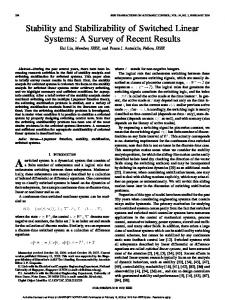
Figure 1: Stability chart with the number of unstable characteristic exponents (NUE) for the system (4)-(6) with τ = 1, a = 0.5 and ka = 0.9 (grey: stable region)

the D-subdivision method, the equation D(iω) = 0 gives the D-curves of the system in the form kp = a, kd ∈ R, if ω = 0. (8) kp = (ω 2 + a) cos(ωτ ) + ka ω 2 , kd =

ω2 + a , if ω ̸= 0. ω sin(ωτ )

(9)

Equation (8) corresponds to static loss of stability (a single real characteristic exponent being equal to zero), while equation (9) is associated with dynamic loss of stability (a pair of complex characteristic exponents with zero real part). The D-curves and the stability chart of the system are shown in Figure 1. It is known that for a given system parameter a, the system √ cannot be stabilized if the feedback delay is larger than the critical value τcrit,PDA = (2 + 2ka )/a (Sieber and Krauskopf, 2005; Insperger et al., 2013). Considering the criteria |ka | < 1, this gives √ 4 . (10) τcrit,PDA = a The case of the PD controller is obtained by setting ka = 0, which gives √ 2 . τcrit,PD = a

(11)

The same feature can be composed in an opposite way. For a given feedback delay, the system cannot be stabilized if the system parameter is larger than a critical value given by 2 4 (12) acrit,PDA = 2 and acrit,PD = 2 . τ τ

3

Finite spectrum assignment

FSA is a predictive control method, which is supposed to realize pole placement for systems with input delay by using a control law that contains a distributed delay

4

term. Time delay compensation is achieved by means of prediction and feedback of the predicted state. In the ideal case, FSA allows the realization of a closed-loop system that operates with a predefined dynamic behavior. Consider a system given in the form of equation (4). In the course of prediction, the controlled system should be described by a model equation, which is called the internal model of the controller. This equation can be written in the form ˜ ˜ ˙ x(t) = Ax(t) + Bu(t − τ˜),

(13)

˜ B ˜ and τ˜ are the estimated system and input matrices and the estimated where A, feedback delay used by the internal model. The predictor used by the FSA approach solves this equation with the initial value x(t − τ˜) and formally shifts the argument of the solution by τ˜. This way the predicted state reads ∫ 0 ˜τ ˜ ˜ A˜ xp (t + τ˜) = e x(t) + e−Aθ Bu(t + θ)dθ. (14) −˜ τ

The controller uses this predicted state for the feedback. Thus the control signal can be written in the form ∫ 0 ˜τ ˜ ˜ A˜ u(t) = Ke x(t) + K e−Aθ Bu(t + θ)dθ, (15) −˜ τ

where K is the control matrix, which contains the control parameters. In case of a second-order system subjected to a PD controller K = ( −kp −kd ). The control law (13) is a linear Volterra equation of the second kind and it involves a distributed delay term. Note that the FSA controller is typically applied to linear systems and does not work for non-linear or non-smooth systems in this form. In the next subsections, the robustness issues of the FSA controller are described for the continuous-time system (4). First, the robustness to parameter mismatches is considered, then the robustness to implementation inaccuracies of the control law is discussed.

3.1

Robustness to parameter mismatches

If the internal model approximates the system parameters with perfect precision (i.e. ˜ = A, B ˜ = B and τ˜ = τ ), then equations (4) and (15) can be reduced to the if A ordinary differential equation (ODE) ˙ x(t) = Ax(t) + BKx(t).

(16)

Thus the feedback delay is eliminated from the control loop, hence the spectrum of the closed-loop system becomes finite and the poles can be shifted to any desired values provided that the pair (A, B) is controllable. This way stability can be achieved for arbitrary system parameters. ˜ ̸= A, B ˜ ̸= B and τ˜ ̸= τ ), If the internal model is not perfectly accurate (i.e. if A then equations (4) and (15) define a retarded functional differential equation (RFDE). ˜ = B, the input u(t) can be eliminated and equations (4) and For the special case B (15) imply ∫ 0 ˜τ ˜ A˜ ˙ ˙ + θ) − Ax(t + θ))dθ, x(t) = Ax(t) + BKe x(t − τ ) + BK e−Aθ (x(t (17) −˜ τ

5

which can be transformed into the RFDE ˜

˜

˙ x(t) =Ax(t) + BKeA˜τ x(t − τ ) + BKx(t) − BKeA˜τ x(t − τ˜) ∫ 0 ˜ ˜ − A)x(t + θ))dθ. + BK e−Aθ (A

(18)

−˜ τ

˜ ̸= B, then differentiation of the control law (15) together with equation (4) give If B the system of RFDEs ˙ x(t) =Ax(t) + Bu(t − τ ),

(19)

˜ ˜ ˜ ˙ u(t) =KeA˜τ Ax(t) + KeA˜τ Bu(t − τ ) + KBu(t) ∫ 0 ˜τ ˜ ˜ ˜ A˜ ˜ − Ke Bu(t − τ˜) + KA e−Aθ Bu(t + θ)dθ.

(20)

−˜ τ

Thus, in case of the slightest mismatch between the internal model and the actual system, the governing equation is an RFDE with infinitely many characteristic exponents. Consequently, finite spectrum assignment in this case is not possible. If the implementation of the control law (15) is perfectly accurate, then stability properties are determined purely by equations (4) and (15). We call this case ideal stability.

3.2

Robustness to implementation inaccuracies of the control law

In order to implement the control procedure in practice, one must perform the online calculation of the integral term in control law (15). Let this integral term be denoted by ∫ 0 ˜ ˜ z(t) = e−Aθ Bu(t + θ)dθ. (21) −˜ τ

One solution for the realization of z(t) is to create a differential equation by deriving equation (21). The differential equation reads ˜ ˜ ˜ ˜ ˙ − τ˜) + Az(t). z(t) = Bu(t) − eA˜τ Bu(t

(22)

It is known that this type of realization involves unstable pole-zero cancellation if matrix A is not Hurwitz, hence it is not capable of stabilizing an unstable system (Manitius and Olbrot, 1979; Mondie et al., 2002; Michiels and Niculescu, 2007). Another way to realize the integral term z(t) is the approximation by a numerical quadrature. In this case the distributed delay term is substituted by a sum of point delays. This way no unstable pole-zero cancellation takes place. An approximation of z(t) by numerical quadrature rule can be given as z(t) ∼ = z1 (t) =

r˜ ∑

˜

˜ − θj,˜r )hj,˜r , eAθj,˜r Bu(t

j=0

6

(23)

where θj,˜r ∈ [0, τ˜], hj,˜r ∈ R and r˜ is an integer approximation parameter so that z1 (t) → z(t) as r˜ → ∞ (Michiels et al, 2003). For instance, a discrete rectangular approximation can be given as z1 (t) =

r˜ ∑

˜

˜ eAj∆t Bu(t − j∆t)∆t,

(24)

j=0

where ∆t = τ˜/˜ r is the discrete time step (i.e., in this case θj,˜r = j∆t and hj,˜r = ∆t). The corresponding control law reads ˜τ A˜

u(t) = Ke

x(t) + K

r˜ ∑

˜

˜ eAθj,˜r Bu(t − θj,˜r )hj,˜r .

(25)

j=0

Although such a realization of the control law is convenient numerically, it presents a limitation in the stability of the closed-loop system. Actually, equations (4) and (25) define a system of NFDEs in the form ˙ x(t) =Ax(t) + Bu(t − τ ), ˜τ A˜

˙ u(t) =Ke

Ax(t) + Ke

˜τ A˜

(26) Bu(t − τ ) +

r˜ ∑

˜

˜ u(t ˙ − θj,˜r )hj,˜r . KeAθj,˜r B

(27)

j=0

As was shown by Mondie et al. (2002), a necessary condition for the stability of the closed-loop system described by equations (4) and (25) is the stability of the associated delay-difference equation (i.e., the difference part of equations (26) and (27)) x(t) = 0, u(t) =

r˜ ∑

(28) ˜

˜ − θj,˜r )hj,˜r . KeAθj,˜r Bu(t

(29)

j=0

In case of r˜ → ∞, the roots of equation (29) converges to the roots of the functional difference equation ∫ 0 ˜ ˜ u(t) = K e−Aθ Bu(t + θ)dθ, (30) −˜ τ

which is obtained by the substitution of x(t) ≡ 0 into the control law (15). Note that equation (30) can be written in the form of the RFDE ∫ 0 ˜τ ˜ ˜ ˜ A˜ ˜ ˜ ˙ e−Aθ Bu(t + θ)dθ. (31) u(t) = KBu(t) − Ke Bu(t − τ˜) + KA −˜ τ

A stable control process can only be obtained if the closed-loop system is stable (i.e., if the RFDE defined by equations (4) and (15) is stable), and if the associated delaydifference equation (29) is stable. In case of r˜ → ∞, this latter condition is equivalent to the stability of the functional difference equation (30). Following Michiels et al. (2003), we call the stability of equations (4), (15) and (30) theoretical stability. It is known that theoretical stability does not imply robust stability with respect to small perturbation of the discretization parameter θj,˜r . As was shown by Michiels et al.

7

(2003), small perturbation of θj,˜r in equation (29) may result in characteristic exponents, whose real parts do not converge to those of equation (30). Consequently, the stability of equations (4)-(15) and (30) is a necessary condition for robust stability, but not sufficient. Actually, robust stability requires the strong stability of the associated delay-difference equation given by equation (29). For the single input case, the necessary and sufficient condition for the strong stability of equation (29) was given by Michiels et al. (2003) as S < 1, where ∫ τ˜ ˜ ˜ Aθ S= (32) Ke B dθ. 0

The restriction by the associated delay-difference equation (both on the theoretical and on the robust stability) can be removed by adding a low-pass filter (Mondie and Michiels, 2003) or by using piecewise constant input, for instance by applying a digital controller (Van Assche et al., 2001; Michiels and Niculescu, 2007).

4

Stability diagrams for ideal, theoretical and robust stability

In this section, domains of ideal, theoretical and robust stability are determined for system (4) with (5) in the plane (kp , kd ). The estimated system and input matrices used by the internal model are assumed in the form ) ( ) ( 0 0 1 ˜ ˜ , (33) , B= A= 1 a ˜ 0 where a ˜ is the estimated system parameter. Ideal stability can be analyzed using the D-subdivision method and Stepan’s formulae (Stepan, 1989) for the characteristic equation of the ideal closed loop system given by equations (4) and (15). For theoretical stability, the stability of the associated functional difference equation (30) should also be determined. Conditions for robust stability can be obtained by the analysis of Eq. (32).

4.1

Stability of the ideal closed-loop control system

Based on equations (5) and (15) the input signal provided by the FSA controller can be given as ( )( ) 1 ch(˜ ατ˜) sh(˜ α τ ˜ ) φ(t) α ˜ u(t) = ( −kp −kd ) α ˜ sh(˜ ατ˜) ch(˜ ατ˜) φ(t) ˙ )( ) ∫ 0( ˜ ˜ 0 ch(˜ αθ) − α1˜ sh(˜ αθ) u(t + θ)dθ, (34) + ( −kp −kd ) ˜ ˜ 1 −˜ αsh(˜ αθ) ch(˜ αθ) −˜ τ √ where α ˜= a ˜, ch and sh indicates cosh and sinh. Here, kp and kd are the proportional and derivative control gains for the predicted state. The solutions for system (4) and (34) are assumed to be in the form φ(t) = φ0 eλt ,

φ(t) ˙ = ω0 eλt ,

8

u(t) = u0 eλt .

(35)

Substitution of expressions (35) into equations (4) and (34) gives the following system of equations   φ0 M(λ) ω0  = 0, (36) u0 where 

−1 λ kp sh(˜ ατ˜) + kd ch(˜ ατ˜) α ˜

λ 2  −α M(λ) = kp ch(˜ ατ˜) + kd α ˜ sh(˜ ατ˜)

 0 −e−λt  , f (λ)

( ) ˜ τ ˜ τ kp e−(λ+α)˜ − 1 −e−(λ−α)˜ +1 f (λ) = 1 + + 2˜ α λ+α ˜ λ−α ˜ ( −(λ+α)˜ ) ˜ τ ˜ τ kd −e + 1 −e−(λ−α)˜ +1 + + 2 λ+α ˜ λ−α ˜ with α =

(37)

(38)

√ a. Hence the characteristic equation of system (4) and (34) reads D(λ) = det(M(λ)) = 0.

(39)

Substitution of λ = iω into equation (39) and decomposition into real and imaginary parts give a linear system of equations for kp and kd in the form ω R(ω) = −(α2 + ω 2 ) + kp sin(ωτ )sh(˜ ατ˜) + kp cos(ωτ )ch(˜ ατ˜) α ˜ ) α2 + ω 2 ( ω + kp 2 1 − cos(ω˜ τ )ch(˜ ατ˜) − sin(ω˜ τ )sh(˜ ατ˜) α ˜ + ω2 α ˜ α2 + ω 2 (−˜ α cos(ω˜ τ )sh(˜ ατ˜) − ω sin(ω˜ τ )ch(˜ ατ˜)) + kd 2 α ˜ + ω2 + kd ω sin(ωτ )ch(˜ ατ˜) + kd α ˜ cos(ωτ )sh(˜ ατ˜) = 0,

(40)

ω cos(ωτ )sh(˜ ατ˜) − kp sin(ωτ )ch(˜ ατ˜) α ˜ ) α2 + ω 2 ( ω + kp 2 sin(ω˜ τ )ch(˜ α τ ˜ ) − cos(ω˜ τ )sh(˜ α τ ˜ ) α ˜ + ω2 α ˜ 2 2 α +ω (ω + α ˜ sin(ω˜ τ )sh(˜ ατ˜) − ω cos(ω˜ τ )ch(˜ ατ˜)) + kd 2 α ˜ + ω2 + kd ω cos(ωτ )ch(˜ ατ˜) − kd α ˜ sin(ωτ )sh(˜ ατ˜) = 0.

(41)

S(ω) = kp

Expressing kp and kd from equations (40) and (41) gives the D-curves for the cases ω = 0 and ω ̸= 0, which can be depicted in the plane (kp , kd ) as shown in panel (a) of Figures 2 and 3. The regions divided by the D-curves are associated with the same number of unstable characteristic exponents (also called instability degree). This number can be calculated by Stepan’s formulae (see Theorems 2.15 and 2.16 in (Stepan, 1989)).

9

kd

kd

kd

kd

(c) 6 (b) 6 (a) 6 (d) 6 4 4 4 4 4 2 0 2 2 2 2 0 S1 2 -4 -4 3 -4 -4 -6 -6 -6 -6 -6 -4 -2 0 2 4 6 -6 -4 -2 0 2 4 6 -6 -4 -2 0 2 4 6 -6 -4 -2 0 2 4 6 kp kp kp kp

Figure 2: Stability chart and the number of unstable characteristic exponents (NUE) of the ideal closed-loop system (a); stability chart and the NUE of the associated functional difference equation (b); robust stability boundaries of the associated delaydifference equation (c); and their superposition (light grey: ideal stability, dark grey: theoretical stability, black: robust stability with respect to implementation inaccuracies) (d) for the system defined by equations (4) and (15) with a ˜ = a = 0.5 and τ˜ = τ = 1

(c) 6 (d) 6 (b) 6 C 4 4 4 NUE=0 4 B 6 S1 A 3 -4 -4 -4 5 -6 -6 -6 -6 -4 -2 0 2 4 6 -6 -4 -2 0 2 4 6 4 6 -6 -4 -2 0 2 4 6 kp kp kp kd

kd

8

kd

kd

(a) 6 4 2 NUE=1 0 0 -2 5 -4 7 -6 -6 -4 -2 0 2 kp

Figure 3: Stability chart and the number of unstable characteristic exponents (NUE) of the ideal closed-loop system (a); stability chart and the NUE of the associated functional difference equation (b); robust stability boundaries of the associated delaydifference equation (c); and their superposition (light grey: ideal stability, dark grey: theoretical stability, black: robust stability with respect to implementation inaccuracies) (d) for the system defined by equations (4) and(15) with a = 0.5, a ˜ = 1.2a, τ = 1 and τ˜ = 1.2τ

10

4.2

Stability of the associated functional difference equation

Substitution of u(t) = u0 eλt and x(t) ≡ 0 into equation (34) gives the characteristic equation of the associated functional difference equation in the form f (λ) = 0,

(42)

where f (λ) is given in equation (38). Substitution of λ = iω into equation (42) and decomposition into real and imaginary parts give ( α ˜ kp kp R(ω) = 2 cos(ω˜ τ )ch(˜ ατ˜) + kd cos(ω˜ τ )sh(˜ ατ˜) − 2 α ˜ +ω α ˜ α ˜ ) kp ω kd ω + 2 sin(ω˜ τ )sh(˜ ατ˜) + sin(ω˜ τ )ch(˜ ατ˜) + 1 = 0, (43) α ˜ α ˜ ( ω kp S(ω) = 2 −k + cos(ω˜ τ )sh(˜ ατ˜) + kd cos(ω˜ τ )ch(˜ ατ˜) d α ˜ + ω2 α ˜ ) kp kd α ˜ − sin(ω˜ τ )ch(˜ ατ˜) − sin(ω˜ τ )sh(˜ ατ˜) = 0. ω ω

(44)

The D-curves of the associated functional difference equation can be given by solving these equations for kp and kd . If ω = 0 then equations (43)-(44) give α ˜ 1 − ch(˜ ατ˜) kp − . α ˜ sh(˜ ατ˜) sh(˜ ατ˜)

(45)

kp =

α ˜ (˜ α2 + ω 2 ) (ω − ω cos(ω˜ τ )ch(˜ ατ˜) + α ˜ sin(ω˜ τ )sh(˜ ατ˜)) , 2 2 2˜ αω − 2˜ αω cos(ω˜ τ )ch(˜ ατ˜) + (˜ α − ω ) sin(ω˜ τ )sh(˜ ατ˜)

(46)

kd =

(˜ α2 + ω 2 ) (˜ α sin(ω˜ τ )ch(˜ ατ˜) − ω cos(ω˜ τ )sh(˜ ατ˜)) . 2˜ αω − 2˜ αω cos(ω˜ τ )ch(˜ ατ˜) + (˜ α2 − ω 2 ) sin(ω˜ τ )sh(˜ ατ˜)

(47)

kd = If ω ̸= 0 then one gets

Since the associated functional difference equation (30) can be written as an RFDE in the form (31), the number of unstable characteristic exponents can be calculated using Stepan’s formula (Stepan, 1989). Note, however, that if the approximation described by equation (23) is used with sufficiently large r˜ to realize the control law, then the associated functional difference equation is a delay-difference equation given by equation (29). If the numerical quadrature is equidistant with time step ∆t = τ˜/˜ r as in equation (24), then the stability of equation (29) is described by r˜ characteristic multipliers µi , i = 1, 2, . . . r˜, each associated with infinitely many characteristic exponents of the form λi,j =

1 1 ln|µi | + i (ωi,0 + j2π), ∆t ∆t

j ∈ Z,

(48)

where ωi,0 is the phase angle of µi so that ωi,0 ∈ (−π, π]. The delay-difference equation (29) is asymptotically stable if all the r˜ characteristic multipliers lie within the unit

11

disc of the complex plane, which implies that all the infinitely many characteristic exponents have negative real parts. If there is a characteristic multiplier with magnitude larger than 1, then it is associated with an infinite sequence of characteristic exponents whose real parts are positive and whose imaginary parts tend to infinity as j is increasing. Consequently, for sufficiently small ∆t, each unstable characteristic exponent of equation (30) corresponds to infinitely many characteristic exponents of equation (29). The D-curves and the number of unstable characteristic exponents of the associated functional difference equation (30) are shown in panel (b) of Figures 2 and 3 for different parameters.

4.3

Robustness to implementation inaccuracies

Expansion of equation (32) gives the condition for the robust stability of the associated delay-difference equation (29) with respect to small perturbation of the discretization parameter θj,˜r in the form ∫ τ˜ 1 S= sh(˜ αθ)kp − ch(˜ αθ)kd dθ. (49) − α ˜ 0 Robust stability is obtained if S < 1 (Michiels et al., 2003). The contour curve defined by S = 1 gives the boundaries of robust stability in the plane (kp , kd ) as shown in panel (c) of Figures 2 and 3. Since S = 0 for (kp , kd ) = (0, 0), the domain of robust stability of equation (29) is the inside of the contour curve.

4.4

Combined stability diagrams

Panels (a), (b) and (c) in Figure 2 show the stability diagram for the ideal closedloop system given by equations (4) and (15), the stability diagram for the associated functional difference equation (30) and the region of robust stability for the associated delay-difference equation (29) for the case when the internal model is perfectly accurate, i.e. when a ˜ = a and τ˜ = τ . Stable domains are indicated by light gray shading. In panels (a) and (b), the number of unstable characteristic exponents for the different parameter regions are also given. Note that for panel (b), each unstable characteristic exponent implies infinitely many characteristic exponents for the actual control system as explained in Section 4.2. The stability condition for the ideal closedloop system (panel (a) in Figure 2) is kp > a and kd > 0, which corresponds to the stability condition for the delay free system. If the approximation described by (23) is used with sufficiently large r˜ to realize the control law, then the region of theoretical stability in the plane (kp , kd ) is reduced to the small triangular shaped region given by the intersection of the stable region of the ideal closed loop system described by equations (4) and (15) and that of the associated functional difference equation (30). The region of robust stability of the closed-loop system with respect to perturbations in the discretization parameter θj,˜r is given by the intersection of the region of theoretical stability and that of the robust stability of equation (29). In panel (d) of Figure 2, light grey, dark grey and black shading denotes different stability properties. Light grey shading denotes the parameters where the ideal closed-loop system is stable, but the associated functional difference equation is unstable, thus the actual control system is unstable for any large r˜ used in the implementation of the control law. Dark

12

grey shading denotes the parameters where both the ideal closed-loop system and the associated functional difference equation are stable (domain of theoretical stability), but the closed loop system is not robustly stable with respect to perturbations in the discretization parameter θj,˜r . Black color denotes the parameters, where the closed loop system is robustly stable with respect to implementation inaccuracies. It is also shown in this figure, that a finite spectrum is achieved only for the ideal closed-loop system in panel (a). If the internal model is not perfectly accurate, i.e. if a ˜ ̸= a and τ˜ ̸= τ , then the spectrum becomes infinite and the stable region shrinks as shown in Figure 3. Figure 4 shows the responses of a robustly stable system with (kp , kd ) = (1, 0), a theoretically stable but not robustly stable system with (kp , kd ) = (1, 1) and an ideally stable but not theoretically stable system with (kp , kd ) = (1.4, 2.2). These three systems correspond to points A, B and C in Figure 3. The simulation was performed by the semi-discretization method with time step h = 0.0025. The initial conditions were φ(0) = 0.05, φ(0) ˙ = 0 and u(θ) = 0, θ ∈ [−τ, 0]. The integral term in the control law was determined by the discrete rectangular approximation according to equation (24), but the time step ∆t was varying periodically over every four steps such that ∆t1 = 0.025, ∆t2 = 0.0275, ∆t3 = 0.025, ∆t4 = 0.0225. This variation presents a special perturbation of the discretization step for the integral in the control law. As can be seen, the ideally stable but not theoretically stable system (point C) is actually unstable due to the unstable difference part of the controller. The theoretically stable but not robustly stable system (point B) is also unstable, since this system is not robust to perturbation of the discretization step in the integral. At parameter point A, the robustly stable system converges to zero after a transient vibration.

5

Application of a digital controller

One technique to overcome the difficulties caused by the sensitivity to implementation inaccuracies of the control law is the application of piecewise constant input (Van Assche et al., 2001; Michiels and Niculescu, 2007). This type of control law corresponds to a digital control system with a sampled output data and zero-order hold, which is widely used in many applications. In this sense, application of digital controller eliminates the restrictions caused by both the approximate implementation of the control law (theoretical stability) and the sensitivity on the discretization rule (robust stability). Stability properties however are still affected by parameter mismatches. In the rest of the paper, therefore, we analyze the stability of the ideal closed loop system in case of non-infinitesimal parameter mismatches between the internal model and the actual system and do not count the issues related to theoretical and robust stability. If a digital controller is applied with sampling period ∆t, then the governing equations read ˙ x(t) = Ax(t) + Bu(ti−r ), t ∈ [ti , ti+1 ), (50) ˜ i) + u(t) = Fx(t

r˜ ∑

˜ j u(ti−j ), Q

t ∈ [ti , ti+1 ),

(51)

j=1 ˜τ ˜ = KeA˜ ˜j = where ti = i∆t (i = 1, 2, . . .), r = ceil(τ /∆t), r˜ = ceil(˜ τ /∆t), F and Q ˜ ˜ ˜ ˜ −A˜τ eAj∆t B∆t. Using state augmentation and the notations ui = u(ti ) and xi = Fe

13

A

0.15

φ

0.1 0.05 0 −0.05 0

B

5

10

15

20

25

t

0.1

30

35

40

φ

0.05 0

−0.05 −0.1

C

0

2

4

6

8

1

2

3

4

0.3

t

10

12

14

16

18

5

6

7

8

9

φ

0.2 0.1 0 −0.1 −0.2 0

t

Figure 4: System response in case of a robustly stable system (A), a theoretically stable but not robustly stable system (B) and an ideally stable but not theoretically stable system (C)

x(ti ), equations (50) and (51) can be written in one of the following forms. If r > r˜ then   xi     ui−1   P 0 ··· 0 0 ··· 0 R  xi+1  ..   ui   F Q  .  ˜1 ··· Q ˜ r˜ 0 · · · 0 0        ui−1   0  ui−˜r  I ··· 0 0 (52)   =  , ui−˜r−1   ..   .. .. .. ..  . .   .   . . . . .   ...    ui−r+1 0 0 ··· I 0  ui−r+1  ui−r

14

where P = eA∆t , R =

∫ ∆t 0

eA(∆t−θ) Bdθ. If r < r˜ then 

      

xi+1 ui ui−1 .. . ui−˜r+1





P  F    0  =   ..   .

0 ˜ Q1 I .. .

0

0

··· ···

0 R ˜ ˜ Qr−1 Qr ··· ... ···

··· ···

0 ˜ Qr˜−1 0 .. . I

xi ui−1 .. .



   0      ˜ r˜  Q   u  i−r+1  0   . ui−r  ..   .   ...   0   ui−˜r+1  ui−˜r

(53)

These equations are of the form yi+1 = Φyi , thus the stability of the system can be determined by the analysis of the eigenvalues of the coefficient matrix Φ, which is actually the monodromy matrix of the discrete-time system. The condition for asymptotic stability reads max(|eig(Φ)|) < 1. (54) In the case of a digital controller, there is no restriction on stability caused by the implementation of the control law, thus the stability can be determined by equation (54) only. In fact, the discrete maps (52) and (53) correspond to the semi-discretization of the original continuous-time system described by equations (4) and (15) with the discretization step being the sampling period ∆t (Insperger and Stepan, 2011). For sufficiently small ∆t, the stability properties of the discrete maps (52) and (53) provide a good approximation of the ideal stability of the original continuous-time system.

6

Analysis of the uncertainties in the parameters

It has been shown that the precision of the approximation of the system parameters used for prediction affects the stability of the system. If a ˜ = a and τ˜ = τ , then the stable region is a quarter plane in the plane (kp , kd ). But in the case when a ˜ ̸= a and τ˜ ̸= τ the stable region shrinks and becomes bounded. This shows that the control procedure is sensitive to the accuracy of the parameters used for the prediction. This sensitivity can be demonstrated on a series of stability charts shown in Figure 5, where different approximation accuracy is used for the system parameter a and for the feedback delay τ . The number of unstable characteristic exponents for the different regions divided by the D-curves are also presented. Remember that here we assume that the control process is implemented by a digital controller, thus the issues related to the theoretical and the robust stability (see Section 4) do not arise. Figure 5 shows that the stability of the control process depends on the accuracy of the parameters a ˜ and τ˜ used by the internal model, which can be characterized by the absolute errors εa = |a−˜ a|/a and ετ = |τ − τ˜|/τ . For a given feedback delay, the critical value of the system parameter a, for which stabilization is just still possible in the presence of given internal model errors εa and ετ is denoted by acrit,FSA . If a < acrit,FSA then there exist a pair of control gains (kp , kd ), which provides a stable control process for any a ˜ and τ˜ satisfying (1 − εa )a ≤ a ˜ ≤ (1 + εa )a and (1 − ετ )τ ≤ τ˜ ≤ (1 + ετ )τ . If a > acrit,FSA then there is no such pair of control gains. Figure 6 presents the critical

15

NUE=1

kd

kd

0

2

6 4 2 0 2 4 6

6 4 0 2 NUE=1 0 2 2 4 6 6 4 2 0 2 4 6 kp

kd

6 4 0 2 NUE=1 0 2 2 4 6 6 4 2 0 2 4 6 kp

8 6 NUE=1

0 2

5

7

4

6 4 2 0 2 4 6 kp 6 4 2 0 2 4 6

8 6

NUE=1 0

4 2

5 7

6 4 2 0 2 4 6 kp

kd

6 4 4 2 0 2 NUE=1 4 0 2 2 3 4 5 6 6 4 2 0 2 4 6 kp

6 4 2 0 2 4 6

6 4 2 0 2 4 6 kp

kd

6 4 4 0 2 2 4 NUE=1 0 2 2 3 4 5 6 6 4 2 0 2 4 6 kp

τ =1.2 τ

τ =τ

kd

kd kd

a= a a =1.2 a

kd

a =0.8 a

τ =0.8 τ

6 4 4 0 2 2 NUE=1 4 0 2 2 4 3 5 6 6 4 2 0 2 4 6 kp

6 4 2 0 2 4 6

8 6 NUE=1

5 7

0

4 2

6 4 2 0 2 4 6 kp

Figure 5: Stability charts and the number of unstable characteristic exponents (NUE) of the system defined by equations (4) and (15) with a = 0.5 and τ = 1 for different accuracy of the internal model parameters a ˜ and τ˜ (grey: stable region)

system parameter acrit,FSA for different errors ε = εa = ετ . The diagram was determined as follows. The absolute errors εa and ετ and the system parameter a were fixed and the 3 × 3 stability charts (similar to the ones shown in Figure 5) were constructed. The system parameter a was said to be robustly stable with respect to the internal model error ε = εa = ετ if there was at least one point in the plane (kp , kd ), which was stable in each of the 3 × 3 stability charts, regardless to the sign of perturbation. If a system parameter a was found to be robustly stable, then it was increased and the same procedure was repeated. The resolution for the system parameter a was 0.01, i.e., a specific value of a = acrit,FSA was said to be critical if it was robustly stable in the sense described above but the same system for a = acrit,FSA + 0.01 was not robustly stable. The concept of this analysis is similar to the stability radius with respect to changes of the system parameters (Michiels and Rose, 2003; Michiels and Niculescu, 2007). The same analysis was performed for the PDA controller described by equations (4) and (6) for different acceleration gains. The results are shown in Figure 6 for comparison. As can be seen, the critical system parameter for the FSA controller decreases

16

Figure 6: The critical system parameter values as function of the internal model error ε = εa = ετ for τ = 1

with increasing internal model error. If the internal model is perfectly accurate (i.e. if ε = εa = ετ = 0) then the theoretical value of acrit,FSA is infinity, hence the effect of input delay is totally compensated. Note that if τ = 1 then the same critical parameter for a PD controller without any parameter uncertainties is acrit,PD = 2 and for a PDA controller it is acrit,PDA = 4. For the FSA controller with small parameter mismatches the achievable critical value of acrit,FSA can be essentially larger than 2 or 4. For large modeling errors, however, delayed state feedback becomes superior to the FSA controller. For instance, for errors ε > 11%, the critical system parameter for the PDA controller with ka = 0.9 is larger than that of the FSA controller. This demonstrates that the FSA controller is more sensitive to modeling inaccuracies than the conventional delayed state feedback. The above observations can be rephrased to the critical delay, too. For a fixed system parameter with small modeling inaccuracies, the FSA controller allows larger feedback delay than the PDA controller. However, for large modeling errors, conventional delayed state feedback becomes superior to the FSA controller.

7

Conclusions

An unstable second-order system was investigated with input delay subjected to a FSA controller. If the parameters of the internal model used for the prediction are not equal to the real system parameters, then the system is described by equations (4) and (15), which define a system of RFDEs involving two types of delays: a point delay τ and a distributed delay term over a delay period of length τ˜. For the ideal continuous-time control system, the stability analysis was performed using the D-subdivision method and the number of unstable characteristic exponents were determined using Stepan’s formula. Stability diagrams were constructed, which present the robustness of the

17

system to parameter mismatches and to implementation inaccuracies of the control law. Here, robustness to implementation inaccuracies is meant in an asymptotic sense, since stability properties are sensitive to arbitrarily small perturbation of the control law (Michiels et al., 2003). This implementation difficulty can be avoided by applying piecewise constant input (e.g., a digital controller). However, in this case, stability properties still depend on the parameter mismatches between the internal model and the real system, although not in an asymptotic sense. The effect of finite mismatches between the internal model and the actual system was analyzed without the effect of the sensitivity to implementation inaccuracies by assuming a digital control system. The stabilizability of the system was investigated for different mismatches through a series of stability charts. The critical system parameter for which stabilization is just still possible in the presence of internal model errors was determined. It was shown that for internal model errors less than 3%, the critical system parameter acrit,FSA is larger than 5, which is already larger than the critical system parameter of a PD or a PDA controller without any parameter uncertainty. For large modeling errors (ε > 11%), however, delayed state feedback was found to be superior to the FSA controller. Thus, the FSA controller extends the limits of stabilization against feedback delay provided that the input signal is available for the control calculation and the system parameters are available with precision less than 11%. Although the current analysis was performed for a second-order system, the FSA controller can be applied to higher-order systems, too. In this case stability properties can be determined in the same way, however, the different modes of the system may interfere with the delay resulting in more intricate stability diagrams. In addition to stabilization, there are other performance measures that a control system should satisfy, such as settling time and overshoot. These measures can also be determined and optimized based on the analysis of the eigenvalues of the coefficient matrix Φ. The settling time is related to the magnitude of the critical eigenvalue, while the system converges to the set point without overshoot if the eigenvalues of Φ are positive real numbers with magnitude less than one.

8

Acknowledgements

This work was supported by the Hungarian National Science Foundation under grant OTKA-K105433. The work reported in the paper has been developed in the framework of the project “Talent care and cultivation in the scientific workshops of BME” project. This project is supported by the grant TAMOP-4.2.2.B-10/1–2010-0009.

References Arstein Z (1982) Linear systems with delayed controls: A reduction. IEEE Transactions on Automatic Control 27:869–879. Bachrathy D and Stepan G (2013) Improved prediction of stability lobes with extended multi frequency solution. CIRP Annals - Manufacturing Technology 62(1):411–414.

18

Bobrenkov OA, Butcher EA and Mann BP (2013) Application of the Liapunov– Floquet transformation to differential equations with time delay and periodic coefficients, Journal of Vibration and Control 19(4):521–537. Breda D, Maset S and Vermiglio R (2012) Approximation of eigenvalues of evolution operators for linear retarded functional differential equations. SIAM Journal on Numerical Analysis 50(3):1456–1483. Duan S, Ni J and Ulsoy AG (2012) Decay function estimation for linear time delay systems via the Lambert W function. Journal of Vibration and Control 18:1462–1473. Engelborghs K, Dambrine M and Roose D (2001) Limitations of a class of stabilization methods for delay systems. IEEE Transactions on Automatic Control 46(2):336–339. Erneux T and Kalmar-Nagy T (2007) Nonlinear stability of a delayed feedback controlled container crane. Journal of Vibration and Control 13(5):603–616. Gawthrop PJ and Ronco E (2002) Predictive pole-placement control with linear models. Automatica 38(3):421–432. Habib G, Rega G and Stepan G (2014) Stability analysis of a two-degree-offreedom mechanical system subject to proportional-derivative digital position control. Journal of Vibration and Control. Epub ahead of print 9 August 2013. DOI: 10.1177/1077546312474014. Hajdu D and Insperger T (2013) Time domain analysis of the Smith predictor in case of parameter uncertainties: A case study. In: August 9, 2013 Proceedings of the ASME 2013 IDETC/CIE, 9th International Conference on Multibody Systems, Nonlinear Dynamics and Control, Portland, OR, USA. DETC2013-12324. Insperger T and Stepan G (2011) Semi-discretization for time-delay systems. New York: Springer. Insperger T, Milton J and Stepan G (2013) Acceleration feedback improves balancing against reflex delay. Journal of the Royal Society Interface 10(79):1742– 5662. Jankovic M (2009) Forwarding, backstepping, and finite spectrum assignment for time delay systems. Automatica 45(1):2–9. Kleinman DL (1969) Optimal control of linear systems with time-delay and observation noise. IEEE Transactions on Automatic Control 14:524–527. Krstic M (2009) Delay compensation for nonlinear, adaptive, and PDE systems. Boston: Birkhauser. Lehotzky D and Insperger T (2012) Stability of turning processes subjected to digital PD control. Periodica Polytechnica – Mechanical Engineering 56(1):33–42.

19

Lehotzky D, Turi J and Insperger T (2014) On the stabilizability of turning processes by digital PD control. International Journal of Dynamics and Control. Epub ahead of print 10 December 2013. DOI: 10.1007/s40435-013-0047-4 Liu L and Kalmar-Nagy T (2010) High-dimensional harmonic balance analysis for second-order delay-differential equations. Journal of Vibration and Control 16(7-8):1189–1208. Loram ID, Gollee H, Lakie M and Gawthrop PJ (2011) Human control of an inverted pendulum: Is continuous control necessary? Is intermittent control effective? Is intermittent control physiological? The Journal of Physiology 589(2):307– 324. Manitius AZ and Olbrot AW (1979) Finite spectrum assignment problem for systems with delays. IEEE Transactions on Automatic Control AC-24:541–553. Masoud ZN, Nayfeh AH and Al-Mousa A (2003) Delayed position-feedback controller for the reduction of payload pendulations of rotary cranes. Journal of Vibration and Control 9:257–277. Maurer C, Peterka R (2005) A new interpretation of spontaneous sway measures based on a simple model of human postural control. Journal of Neurophysiology 93:189–200. Michiels W and Niculescu S-I (2007) Stability and stabilization of time delay systems – An eigenvalue based approach. Philadelphia: SIAM Publications. Michiels W and Roose D (2003) An eigenvalue based approach to the robust stabilization of linear time-delay systems. International Journal of Control 76(7):678– 686. Michiels W, Mondie S and Roose D (2003) Robust stabilization of time-delay systems with distributed delay control laws: Necessary and sufficient conditions for a safe implementation. Technical Report of Department of Computer Science, Katholieke Universiteit Leuven, TWReport 363. Milton J, Cabrera JL, Ohira T, Tajima S, Tonosaki Y, Eurich CW and Campbell SA (2009) The time-delayed inverted pendulum: Implications for human balance control. Chaos 19:026110. Mondie S and Michiels W (2003) Finite spectrum assignment of unstable timedelay systems with a safe implementation. IEEE Transactions on Automatic Control 48:2207–2212. Mondie S, Dambrine M and Santos O (2002) Approximation of control laws with distributed delays: a necessary condition for stability. Kybernetika 38(5):541–551. Moss F and Milton J (2003) Balancing the unbalanced. Nature (London) 425:911– 912.

20

Munoa J, Mancisidor I, Loix N, Uriarte LG, Barcena R and Zatarain M (2013) Chatter suppression in ram type travelling column milling machines using a biaxial inertial actuator. CIRP Annals - Manufacturing Technology 62(1):407–410. Olgac N and Sipahi R (2002) An exact method for the stability analysis of time delayed LTI systems. IEEE Transactions on Automatic Control 47:793–797. Orosz G, Wilson RE, Szalai R and Stepan G (2009) Exciting traffic jams: Nonlinear phenomena behind traffic jam formation on highways. Physical Review 80:046205. Palmor ZJ (2000) Time-delay compensation: Smith predictor and its modifications. In: Levine W (ed) The Control Handbook, Boca Raton: CRC and IEEE Press, pp. 224–237. Qin ZC, Li X, Zhong S and Sun JQ (2014), Control experiments on time-delayed dynamical systems. Journal of Vibration and Control. Epub ahead of print 11 December 2012. DOI: 10.1177/1077546312469424. Sieber J and Krauskopf B (2005) Extending the permissible control loop latency for the controlled inverted pendulum. Dynamical Systems 20(2):189–199. Smith OJM (1957) Closer control of loops with dead time. Chemical Engineering Progress 53(5):217–219. Stepan G (1989) Retarded dynamical systems, Harlow: Longman. Stepan G (2001) Vibrations of machines subjected to digital force control. International Journal of Solids and Structures 38:2149–2159. Stepan G (2009) Delay effects in the human sensory system during balancing. Philosophical Transactions of the Royal Society A 367:1195–1212. Sun JQ (2009) A method of continuous time approximation of delayed dynamical systems. Communications in Nonlinear Science and Numerical Simulation 14:998–1007. Suzuki Y, Nomura T, Casadio M and Morasso P (2012) Intermittent control with ankle, hip, and mixed strategies during quiet standing: A theoretical proposal based on a double inverted pendulum model. Journal of Theoretical Biology 310:55–79. Van Assche V, Dambrine M, Lafay J-F and Richard J-P (2001) Implementation of a distributed control law for a class of systems with delay, In: Proceedings of the 3rd Workshop on Time Delay Systems, pp. 266–271. Wang QG, Lee TH and Tan KK (1999) Finite spectrum assignment for time delay systems. London: Springer. Zatarain M and Dombovari Z (2014) Stability analysis of milling with irregular pitch tools by the implicit subspace iteration method. International Journal of Dynamics and Control. Epub ahead of print 15 January 2014. DOI: 10.1007/s40435-013-0052-7.

21

Zhang XY and Sun JQ (2014) A note on the stability of linear dynamical systems with time delay. Journal of Vibration and Control. Epub ahead of print 12 April 2013. DOI: 10.1177/1077546312473319.

22