On the semantics of continuous quantities in ... - Semantic Scholar

On the semantics of continuous quantities in natural languages Shenghui Wang, David E. Rydeheard and David S. Br´ee∗

Abstract We investigate the semantics of continuous quantities such as colour and shape as they occur in natural languages. To do so, we introduce a mathematical framework which allows us to define semantics uniformly across many different continuous quantities. The original motivation for this was the analysis of texts in descriptive sciences and we begin a series of experiments testing proposed semantic interpretations against these texts and the natural phenomena being described. Finally, we describe computational applications of the semantics in information processing.

1

Introduction

We have difficulty expressing continuously variable quantities in natural languages – the variability defeats all attempts at a vocabulary. Consider, for example, the words and phrases by which we try to capture the infinite variation in colour. And colour is easy! – easy in several technical senses. Consider attempting to describe the shape of objects. The range of variation and its complexity mean that any simple vocabulary and formation of compound phrases can only loosely capture the real shape of objects. Other quantities are similar: for example, sounds and textures, expressions describing spatial arrangements, and temporal expressions describing and comparing sequences of events in, for example, life histories. The way we build expressions in natural languages for describing continuous quantities is the same over a wide range of such quantities. There is a common terminology, independent of the quantity under consideration, for describing, for example, ranges of values, intermediate values, modified and transformed values, proximity and equivalence of values, combinations of values of several different quantities, and logical expressions involving values and ranges. In this paper, we investigate the proposal that not only is there a common terminology across continuous quantities, but also a common semantics of these expressions. That is, there is a semantics not simply of particular phrases, but a generic account giving a meaning to each phrase formation independent of both the choice of quantity we are describing and the choice of model for interpreting a particular quantity. Different interpretations arise from different choices of model but each via a uniform schema of interpretation. Our interest in this topic arose from a practical problem. In the descriptive sciences, such as botany (our primary example), there are large corpora of written knowledge. School of Computer Science, The University of Manchester, Oxford Road, Manchester M13 9PL, U.K. Email addresses: [email protected], [email protected] and [email protected]. ∗

1

In botany, in particular, there is a vast collection of parallel (and often independent) descriptions with the same species described by many different authors. These written descriptions have a degree of precision and detail not normally encountered in texts. Expressions for continuous quantities form a major component of these descriptions, for example, expressions for flower colour, leaf shape, arrangement of parts, petal texture, stem cross-sections, vein patterns, etc. and also a wealth of temporal and spatial expressions. Because of the large amount of botanical text, it is tempting to try to automate some of the analysis. With such an automation, we can compare different descriptions to assess how much they agree and combine them into an integrated form, we can collate and compare knowledge across times and geographically, and we can provide computational tools for information organisation and retrieval. However, to achieve all of this, we need to analyse the constituent descriptions, which are primarily descriptions of continuous quantities, and this analysis requires a suitable semantics – hence the topic of this paper. Although this analysis originated in the rather recondite area, from a linguistic point of view, of botanical terminology and descriptive floras, it has led to the results of this paper in which we address general issues in the semantics of natural languages, in particular, in the structure of semantics and the generality of semantic description, as well as the form of semantic models and techniques for constructing and evaluating models. Because botany, as one of the premier descriptive sciences, offers a wealth of material on which to test and develop this analysis, we shall use botanical examples throughout this paper, but alert the reader to the fact that we are, in fact, undertaking a general analysis of a topic in natural language semantics, relying on botanical sources to provide example texts, together with a degree of precision of description which we can use to evaluate models. The uniform approach to modelling which we describe here is based on a choosing a suitable mathematical structure for models. It turns out that metrics and topology provide what appears to be a workable basis for the semantics of continuous quantities. We are not the first, of course, to propose the use of metric spaces as models, indeed there is a considerable history and expanding body of work in this area. What we do however is propose a uniform structure for the semantics of continuous quantities and, moreover, show how we may test this proposal against nature itself and also against the semantic information derived from the statistical analysis of word use in texts. As examples of the way that semantics may be formulated and evaluated, we consider two continuous quantities which differ considerably in the variation they exhibit and in their modelling: these are (1) simple shapes and (2) colour. Finally, we describe computational applications of this modelling to text-based information retrieval and integration, and to the interrogation and organisation of databases. All of this is very much experimental and we see this paper as a series of experiments in practical semantics. As for other work in the area, there has been considerable interest in the way that spoken languages handle colour terms and the linguistic implications of this, including identifying ‘language universals’, (see the bibliography (Byrne & Hilbert 1997) for details). There has also been work on the automated processing of text, handling colour (Dowman 2001) or shape terms, and work on database aspects of storing and retrieving information based on semantic ideas including those of colour and shape (see, for example, (MarchandMaillet 2006)). Metrics have been proposed in various approaches to semantics, including in the work on ‘conceptual spaces’ (see e.g. (G¨ardenfors 2000), which uses some techniques similar to those in this paper but applied to the broader problem of the relationship between concepts and language), spatial expressions (see e.g. (Schwering 2005), (Schwering 2

& Raubal 2005) and (Egenhofer & Shariff 1998)) and programming language semantics (see e.g. (de Bakker & de Vink 1996)). The relatively new field of morphometrics covers the measurement and analysis of size and shape in nature and its consequences in taxonomy and phylogeny, see for example (Bookstein 1991), (Dickinson, Parker & Strauss 1987), (Marcus, Corti, Loy, Naylor & Slice 1996), (Rohlf & Marcus 1993). Automated analysis of botanical texts is of considerable current interest, see, for example, (Lydon, Wood, Huxley & Sutton 2003), (Wood, Lydon, Tablan, Maynard & Cunningham 2004), (Wood & Wang 2004), (Wood, Lydon, Tablan, Maynard & Cunningham 2003), (Keet 2003) and (Wang & Pan 2005). A website is available (Rydeheard & Wang 2006) containing material and numerical data gathered to support the analysis of semantics which we present in this paper.

1.1

Descriptive sciences

As a source of expressions for continuous quantities, we turn to the descriptive sciences, in particular, to botany. Botanists describe plants in so-called floras. We use floras in English, though others are available, including in Latin. The description of taxa (groups of plants) uses a combination of standard English, specialist terminology, abbreviations and numerical expressions. For example, chosen fairly much at random from (Clapham, Tutin & Warburg 1973) is Veronica anagallis-aquatica, Water Speedwell: Perennial or sometimes annual, glabrous except for the sometimes glandular infl. Stems 20-30 cm., fleshy, green, shortly creeping and rooting below, then ascending. Lvs 5-12 cm., ovate-lanceolate or lanceolate, acute, half-clasping, remotely toothed. Racemes in opposite pairs, rather lax, 10-50-fld., ascending. Bracts linear, acute, shorter than or equalling the fl.-stalks at flowering. Calyxlobes ovate-lanceolate, acute. Corolla c. 5-6 mm. diam., pale blue. Fl.-stalks ascending after flowering. Capsule ±orbicular, usually slightly longer than broad. Fl. 6-8. In ponds, streams, wet meadows and on wet mud. Common throughout much of the British Is. For those not familiar with botanical texts, the only specialist terminology we explore in this paper is that of leaf shape and we include a glossary of some of the commoner terms (Appendix B) and a small ‘picture gallery’ in Figure 3. Extensive glossaries and definitions of terms for vascular plants are available (see, for example, (Stearn 2004) and (Massey & Murphy 1998)). Botanists bring several hundred years’ experience to these descriptions and also a refined use of terminology. Often, over the years, a substantial number of different descriptions have been provided for a taxon (and the delimitation of taxa have changed, but that is not usually a linguistic problem). This provides a wealth of textual sources for descriptions of continuous quantities in a precise domain and enables us to ask about the exact meaning and equivalence of descriptions. Our analysis of such texts and their use of continuous quantities has thus three distinct ingredients: (1) the texts themselves, including a range of different texts covering the same taxon, (2) the plants (for primary material, we have used both the resources of The University of Manchester Herbarium and field collections), and (3) the mathematical modelling of continuous quantities. It is in the interaction between these three components 3

that we find a precise analysis of the semantics, comparing real data with mathematical models and the precision and imprecision of botanical texts.

2

Descriptive phrases for continuous quantities

We begin by looking at some of the phrase formations in English for describing continuous quantities, and consider semantic aspects of these phrases.

2.1

Basic terms

Consider words describing particular values of continuous quantities, for example blue for colour, or ovate for leaf shape (see Appendix B for definitions of some leaf shapes and Figure 3 for some pictures). What do these denote? We shall use the standard semantic brackets for the denotations: thus, what kind of objects are [[blue]] and [[ovate]]? Are these single objects in the space of semantic objects, or, noticing that these terms may cover a variety of ‘close’ colours or shapes, perhaps the denotations are regions in the space? If so, how do we determine the location and shape of these regions? Does it differ for different ‘domains of discourse’ and for different models of colour or of shape? For domains of discourse, we may expect different interpretations for different domains. For example, blue for flower colour may be something different from blue in renaissance painting!

2.2

Ranges and intermediates

Consider phrases such as, for colour, pink to purple or, for leaf shape, ovate to elliptic. What are the following semantic objects: [[pink to purple]] or [[ovate to elliptic]]? Clearly, they are a delimited range of values between the end-points. But which values are in the ranges given? How red does pink have to be before it steps outside the range of colours in pink to purple? Is lanceolate in the range linear to elliptic? The answer to the latter, perhaps, ought to be no, but then what aspects of a shape determine this? Is the range pink to purple the same whatever the domain of discourse or does it vary? Can we interpret yellow to blue, and if not why not? Is the range of colours a ‘path’ in the space of semantic objects, or is it a region, and how is it determined by the meaning of the end-points? If there is such a determination for colours, could it be the same determinant for shape, e.g. determining the range of shapes described by ovate to elliptic? A related form of phrase commonly used is violet-blue or, for shape, ovate-lanceolate. These phrases are usually used to denote a particular colour and a particular shape, each an intermediate between the two values. But where is this intermediate to be located? Is it related to the above description of ranges, i.e. is an intermediate in the range, and if so which point? How far along the range should we travel to locate the intermediate and is this the same whatever the end-points, and whatever the quantities under consideration and whatever the model?

2.3

Modifiers

Consider phrases such as pale yellow or deep reddish purple, or, for shape, broadly elliptic or narrowly linear. Each of these uses a modifier to change the denotation of the adjective. We may ask similar questions to those above about the semantic objects [[pale yellow]] or [[broadly elliptic]]. Clearly, [[pale]] and [[broadly]] are operators or transformations on the 4

space of colours and leaf shapes, respectively. This is not ‘compositionality’ of semantics but merely a statement that [[pale]] and [[broadly]] transform colours to colours and shapes to shapes. However, we may ask: is the transformation [[pale]] of colours uniform in any sense i.e. does it ‘do the same thing to each colour’, likewise is [[broadly]] a uniform transformation of shape? We may also ask more subtle questions, such as: if two colours are in some sense close, then when transformed by [[pale]] are the resulting colours close? How is this related to the fact that, physiologically, we are better at distinguishing greens than reds? There are several related questions here: (1) is there any sense in which these transformations are continuous, and (2) are they isometries i.e. preserving ‘distances’ ? Continuity is interesting because it is related to our own perceptual ability to distinguish between, say, colours, and the way that semantics should reflect this limiting property.

2.4

Mixed forms

Another form of expression for continuous quantities is common: those which mix several types of quantity. These occur especially in trying to describe the complex variation that is often present in nature, where the variation of one quantity depends upon other quantities. Examples of this are (combining colour and frequency) violet-blue, rarely pink or white, or (combining shape and frequency) usually broadly ovate, occasionally deltoid, or (combining position with shape) lvs oblong-ovate to lanceolate, narrowing up the stem, or (combining position and size) lower lvs large, upper smaller. Each of these combines two quantities (indeed it would be possible to combine colour and shape – e.g. when petals display different shapes with different colours). These expressions deal with pairs of quantities which may be combined as though they were a single quantity. The key to interpreting these expressions lies in the way that the two quantities interact, for example, in the above expression for leaf shape variation with position on the stem, a full description would capture the functional relationship between narrowness of the leaves and position on the stem.

2.5

Logical operations

Logical operators naturally occur in the description of continuous quantities and the complexity of their variation. Disjunction is common, for example, obovate to narrowly elliptic or narrowly obovate, or violet-blue, rarely pink or white. In our automated analysis of botanical texts, we find that the word and is rarely used as a simple conjunction of values, but instead occurs in contexts such as, narrowly spatulate to linear-spatulate and rounded combining different quantities, or in attempting to indicate where variation occurs, for example, with numerous oblong and elliptic small lenticels (with and often indicating that on individual specimens two or more values coexist). Negation is rare and almost entirely confined to distinguishing between close taxa. Interpreting values as regions of space, logical operators, in particular disjunction, combine regions of space. Do the standard set operations correspond to the semantics of these expressions? What are the extended regions that now correspond to semantic objects? What sort of reasoning is associated with this logic and is it automatable, for example, for incorporation in description logics for database structuring and querying?

5

Finally, when presented with different descriptions of the same taxon, do logical operators provide suitable combined descriptions for integrating the information?

2.6

Equality, separation, and degrees of semantic equivalence

When looking at different (independent) floras describing similar collections of species one is struck by the fact that rarely do they lexically agree – rarely is the same phrase used to describe the same attribute of the same species in different floras. For example, the shape of the leaves of Quercus robur (Pedunculate Oak) is described variously as: obovate to narrowly elliptic or narrowly obovate obovate to narrowly elliptic usually obovate oblong obovate to elliptic oblong, usually broadest at the base oval oblong to widest above the middle obovate-oblong. Similarly, the petal colour of Origanum vulgare (Wild Marjoram) is variously described as: violet-purple white or purplish-red pink purple-red to pale pink reddish-purple, rarely white. The question then is: do these descriptions agree or disagree and can we quantify the amount or range of agreement and disagreement? This is entirely a semantic question: how do semantic objects capture the amount of agreement? Notice that there may be semantic disagreement for various reasons: the delimitation of taxa (e.g. species) may be different so that a specimen may be allocated to one species by one author and to another species by another, or the natural range of variation within a species observed by different authors may be different (neither of these apply to the well-known species above – except possibly some regional variation for O. vulgare), or the use of terms and phrases may vary from author to author, as may the degree of precision considered necessary by authors. We would expect a semantics to be able to distinguish actual disagreement from different but equivalent descriptions. Thus, for two phrases, P 1 and P2 , we are asking, in a strict form, whether [[P1 ]] = [[P2 ]], and thus, what is equality of semantic objects? However, for phrases describing continuous quantities, exact equality is likely to be too fine a distinction and a notion of proximity (closeness) is more likely to be applicable – so again we appear to need some notion of distance or closeness. Moreover, for phrases describing regions of the space and paths within it, we need to consider (1) the equivalence of regions and of paths, (2) a notion of closeness which is applicable to regions and to paths, and (3) have a way of assessing the degree of overlap 6

between two regions and between two paths. These are clearly more complex aspects of the structure of the semantic spaces, but are essential to the processing of multiple parallel texts and assessing their degree of consistency. Given such multiple descriptions of the same aspect of the same taxon, an important question is: how do we combine them into a joint description? This is the process of data integration and clearly requires the semantic considerations just listed to produce a suitable combined form which captures the overall information. This combined form should (1) have an explicit relationship with the source expressions, (2) avoid redundancy, (3) detect and report any inconsistency that is present, and finally, (4) properly take into account qualifications such as frequency or variation with habitat, etc. We will discuss how to automate this process of integration later in the paper (in Section 8).

2.7

Ambiguity

Related to the question of equivalence of interpretations is the identification and resolution of ambiguity (phrases having two or more different interpretations in a model). Descriptions of continuous quantities are often complex because of the variation that we wish to describe. Thus even pink to purple or blue is open to two interpretations (which some botanists are careful to distinguish), and more complex combinations of values, ranges and logical connectives are often a source of hidden ambiguity. Another source of ambiguity lies in determining where variation occurs. For example, flowers pink to purple has three possible readings: (1) some flowers are multicoloured in this range, (2) some plants have flowers which each have a single colour but vary from flower to flower, and (3) plants have uniformly coloured flowers, but different plants have different colours. Also, flowers can change colour with age, so there may be a temporal element to the variation. Ambiguity also arises in the description of continuous quantities because of the presence of ‘vagueness’ or ‘underspecification’. This vagueness is present in the imprecise (or nonexistent) definition of terms and in the way that terms are used, and also in the use of phrases to denote ranges of values, ranges which themselves are unspecified. For some quantities, such as colour and leaf shape, there are ‘naming schemes’ or glossaries which define terms as points or regions in models. To what extent these definitions contribute to a suitable semantics is one of the issues we address in this paper. A further aspect of ambiguity is that a numerical semantics, allocating particular numbers to expressions describing continuous quantities, will in general be too fine-grained, that is, it will distinguish semantic objects that we wish to consider equivalent. We thus introduce a spurious ambiguity which is an artifice of the modelling technique. Since the intended interpretations are not always precise, it may not be clear whether a phrase is inherently ambiguous or whether it is an artifice of the modelling. The approach we adopt to making the granularity of the semantics match the intended meaning is to equip the models with a notion of proximity between semantic objects, so that as well as asking whether two objects are equal we can ask how close they are, and therefore quantify the ‘degree of ambiguity’.

3

Evidence

When proposing a semantics for phrases in a natural language, it is often considered sufficient to justify the semantics by the degree of correspondence between the formal 7

meaning and ‘what we know the phrase means’. After all, the latter is always informal and a formal semantics is nothing if it doesn’t correspond (in a necessarily unstated way) with what we know the phrases mean. Of course, the success of such semantic description depends on much more than this, for example on the elegance of the modelling, on the way that compound meanings are assembled, on algebras for manipulating meaning, on the way that equivalence of meaning can be assessed, and on a range of computational and complexity issues, including the computation of meaning for particular phrases, and the computation of equivalence and proximity of meaning. However, in the generic account which we are to give, we cannot rely on a simple appeal to ‘what we know the phrase means’ to justify its correctness. This is because we are proposing, for each type of phrase formation, a common interpretation across a wide range of quantities and models. Moreover, the quantities we are dealing with are measurable with numerical descriptions of various kinds. We will show how we may gather empirical evidence to support each individual interpretation, and provide accumulating evidence for the greater claim that, by choosing appropriate models, such interpretations are uniform across a range of different quantities. Firstly, we may test the semantics directly against nature. For example, using measurements of leaf dimensions and flower colour in the field, or from herbaria, or from photographs, we can gather data and compare them with descriptions in flora and the proposed semantics of these descriptions. If a flora describes a species to have leaves lanceolate to ovate, we can actually measure a sample of leaves and see whether the proposed paths in the semantic model include these actual leaf shapes. Colour is a little more difficult, though possible, in terms of direct measurement. Ideally, one would analyse the reflected light and convert this into one of the colour models to see whether the interpretation matches our perception of this light. A test that is simpler to undertake is to analyse the pixels in digital images and compare these with those predicted in the semantics. A great deal of conversion of formats and colour correction is involved in taking a digital photograph, and storing and displaying the image, so that there may be considerable distance between the light from flowers and the colour coding in the final digital image. However, this provides simple access to some data, and we have undertaken a preliminary analysis and report the results later in this paper. Secondly, we can analyse texts to provide support for the semantics. There are several aspects to this. One may analyse individual floras, or even large botanical corpora, to gather statistical data about word use, occurrences and contexts. For botanical texts, there is additional evidence provided by the fact that we have multiple parallel descriptions (not always independent – a fact that may be taken into account). For example, there are many floras of the British Isles describing many of the same species. By comparing descriptions of the same attributes of plants across different accounts we may evaluate notions of proximity and equivalence and the implications of this for creating and comparing semantic models. In this paper, we begin this analysis by presenting a number of experiments showing how the proposed semantics may be evaluated. More exhaustive evaluation would require quantities in addition to leaf shape and colour, more field data, sources other than botanical texts, and finally, more formal measurements to support the evaluation of the semantics. It may have occurred to the reader that, whilst such empirical methods may provide some data to support a proposed semantics, there is a more fundamental aspect so far unmentioned, namely that a generic semantics ought to be inherent in the very concepts 8

and language that we use to describe continuous quantities. For example, in describing a range of colours as pink to purple, the semantics is determined by the processes that one uses to formulate this phrase and which the hearer/reader uses to analyse it. Granted, our use of such phrases can be fairly vague and there may be some disagreement about exactly which colours are in this range. Nevertheless, in formulating such a phrase, one clearly intends it to have a meaning, precise or imprecise though it is. Where does this meaning come from? Is it related to, say, our childhood experience of mixing paints, or to some other notion of the way that colours transform themselves into other colours? This is not like asking how we acquire the meaning of, say, red, since we can put together entirely new phrases for colour ranges, and still have an intended (and often understood) meaning. The stronger suggestion here is that we may use a similar way of providing a meaning to such phrases whether it be for colour, shape or other continuous quantities. Is there a general conceptual argument for this? The answer to this lies in the notion of the ‘appropriateness’ of a model, that is, how we choose to construct semantic models. Models can have a degree of appropriateness for their role in semantics built into their construction. Such models are then adequate for the task and properties of the space really do correspond to a semantic reality which we can compare with the physical phenomena under discussion. We shall see this in action shortly with both shape and colour models. Finally, a word of warning: Scientists in various disciplines have accumulated several centuries of experience devising textual descriptions and ways of incorporating a relevant degree of precision into these descriptions. Testing semantic schema using such texts should therefore be a rigorous and precise undertaking. However, whilst the texts may provide some of the best empirical evidence to support the semantics, the precision of this support, as we shall see, often falls below the precision that we may express in the semantics. The reasons for this are several: (1) the texts are in natural languages and so, whilst some of the terms may have technical and precise descriptions, others, both simple adjectives and the crucial linking phrases are undefined and rely on our ‘common understanding’ of these terms, (2) texts in descriptive sciences describe with appropriate precision for their aims, thus a flora may distinguish between two species on flower colour, say red and blue, without any need to be more precise (e.g. wavelengths of light!), and finally, (3) some aspects of nature can be extremely variable and a real attempt to capture the full range and intricacy of variation in a descriptive phrase is beyond the purposes of such texts. Thus the precision of the semantics calculated below will not always be reflected by the precision of data gathered from nature and the precision of description in the texts.

4

Metric semantics

We now describe a mathematical semantics of expressions for continuous quantities in natural languages. We interpret phrases in metric spaces. In order not to interrupt the development of the semantics, we have gathered the required elements of metric space theory in an appendix to this paper (Appendix A). Most of this material is standard and may be found in textbooks (e.g. (Giles 1987) or (Copson 1968)), though the emphasis in texts can vary and important concepts in metric semantics may not appear. The key concepts from metric space theory that we draw on for a description of the semantics of continuous quantities in natural languages are:

9

• a notion of proximity or closeness of semantic values, • definitions of regions of space determined by proximity, and measures of similarity and dissimilarity between regions, • continuity of maps between spaces, • paths, especially shortest paths (often called ‘geodesics’), between pairs of points, and finally, • products of spaces. Metric spaces may not be the only setting for the semantics of continuous quantities. However, in this paper, we show that they do provide workable models of sufficient generality. The definition of a semantics for expressions is a two stage process: 1. Define how each phrase form for continuous quantities is interpreted in an arbitrary metric space, 2. Choose appropriate spaces, and interpretations of basic terms, to model each particular quantity. Combining these two then provides a semantics of expressions for a particular continuous quantity. In this section, we deal with the first process, and in later sections show how appropriate models may be chosen.

4.1

Denotations

Points in a metric space are the location of exact values. For continuous quantities, as they occur in nature or as described in natural languages, collections of points rather than single points are the appropriate denotation for phrases, allowing points close to and indistinguishable from each other to be collected together in the denotation. Thus words and phrases describing continuous quantities are interpreted as regions of a metric space. Another reason for considering regions is that some expressions denote ranges of values, either around a point, or between two or more points, and the natural interpretation of these is as regions of the space. Determining the location, extent and shape of regions which correspond to phrases is, however, often difficult and raises a number of general issues about natural language semantics. The key problem is the under-specification that is present in our use of language. This vagueness which occurs in most description, even for texts in the descriptive sciences, means that regions are rarely determined precisely. For a few quantities, there are accepted definitions of regions and with suitable models these may be encoded as subsets of metric spaces. We will consider cases of this later when we look at metric models of leaf-shape descriptions and of colour. More commonly, definitions of terms (if they exist at all) describe values rather than regions in a modelling space – these are often called ‘prototypical values’. Given such a scheme how do we determine the regions which correspond to terms? As we move away from a denoting value for a term, how far can we proceed before we are outside the denotation of the term? This is clearly a key question about meaning – the equality and extent 10

of denotations. Several approaches have been proposed in the literature. Once a suitable model has been determined and a metric defined on the points, one possibility is to define the region determined by a denoting value, as the set of all points closer to this value than to other denoting values (thus producing the, so-called, Voronoi diagram of the values). Whilst this technique has been proposed for certain naming schemes, it clearly suffers several shortcomings: the introduction of new terms changes the denotation of existing terms, and unless the naming scheme covers the space uniformly and with a sufficiently fine granularity, such regions may well include points which are not part of the denotation. Another problem is that some names may be more general than others (e.g. yellow may include pale yellow and golden yellow) in which case we produce a hierarchy of regions under inclusion. It is possible to extend the concept of the Voronoi diagram to this case if each term has a level in the hierarchy and the terms cover the space appropriately at each level. Other approaches attempt to give a fixed, or varying, granularity to the denotations so that the boundaries of regions are given by (often simple) rules for allocating distances from points within which the denotation is valid. Considerable work has been done on methods of identifying regions corresponding to basic terms for describing colours (which we discuss in Section 7). Rather than relying on identifying boundaries of regions, some approaches propose a ‘graded membership’ of sets i.e. ‘fuzzy sets’, often related to metrics (see (Lammens 1994), (Belpaeme 2001b), (Belpaeme 2001a) for discussions of this approach for the semantics of colour). A question of a rather different kind, is not how to determine particular denotational regions, but what types of subsets are valid as denotations, i.e. what properties of subsets do we expect denoting regions to have? It turns out that we need not be prescriptive about the subsets that serve as denotations. However, there are some ‘natural’ properties which reflect the way that metric spaces function as models. In addition, some constructions and forms of computational representations require that the subsets satisfy certain properties. Some of the relevant properties are: (1) that subsets are are closed, bounded and nonempty. For such subsets, certain distances between them are defined (Hausdorff distances). When subsets are not closed, we may of course, consider their closure; (2) that subsets consist of a finite number of disjoint path-connected subsets. The denotations we define are of this form, and we use this as a means of building computational representations of denotations in multidimensional spaces. Computing with regions as denotations rather than points makes for additional complication in the definition of semantics. For example, how do we determine the similarity between semantic values when these values are regions? For regions, similarity has several aspects: the regions are of similar shape with a similar orientation, and that they occupy a similar location. Various notions of similarity of regions in metric spaces have recently been proposed, with different applications looking at different notions of similarity (see, for example, (Veltkamp & Hagedoorn 2001)). The theory of metric spaces provides several notions of distances between regions (see Appendix A), which we investigate later to see to what extent they reflect semantic proximity. From a computational viewpoint, we need both a representation of regions and the ability to calculate an appropriate distance or similarity measure between regions. We may then compute semantic functions, compare descriptions to assess, for example, proximity and consistency, and automatically ‘integrate’ multiple parallel descriptions into a single form. We have experimented with representations of regions as delimited ranges of parameters in multidimensional spaces, and simple similarity measures. This provides 11

successful computational results for certain models, but, in general, more complex representations are required, depending upon both the construction of the space and its metric. We look at these issues later in the paper.

4.2

Basic terms

Semantic functions for expressions for continuous quantities are built from denotations of basic terms, which include individual denoting words such as red or ovate, and individual modifiers, such as yellowish, or pale, or, for shapes, narrow etc. Given these basic denotations, we define semantic functions by showing how to construct denotations of compound phrases. The latter is where we consider generic constructions: for each phrase formation, a single construction for all quantities and choices of modelling spaces. We begin with the denotations of basic terms. Where do these come from? The shape, location and extent of basic regions clearly depends on quantity being modelled and the modelling space as well as the precision of the descriptive term. For some quantities, there are ‘glossaries’ which describe the meaning of basic terms, often in a fairly imprecise manner. For example, for leaf shapes, Stace (1997) and Massey & Murphy (1998) not only describe typical values (as is often done simply with pictures) but also delimit appropriate (but different) regions of the space. As mentioned above, for other quantities, there are more systematic descriptions of basic terms via ‘naming schemes’. For example, there are colour naming schemes allocating to basic colour terms, values in a model, and, for many schemes, appropriate regions of a model (these are referenced later, when we look at colour models in Section 7) However, for many quantities, there are no established definitions for the basic terms, in which case we may attempt to devise our own definitions, and then evaluate the correctness of the consequent semantics using methods that we describe later. Of course, the structuring of the semantics means that semantic definitions are parameterised over these basic interpretations, and so we may test various interpretations of basic terms within a fixed semantic framework.

4.3

Ranges and intermediates

Consider ranges of values of the form A to B. A natural interpretation of these is in terms of paths in a metric space i.e. continuous maps from a closed interval of real numbers into the space (see Appendix A for definitions). What paths are we to use as the denotation of ranges? One of the claims we make in this paper is that, with an appropriate choice of model, the requisite paths for ranges are shortest paths, also known as geodesic paths, in the space. This choice of paths is not as arbitrary as it may first appear. In the constructions of models for various quantities, we will show how metrics may be chosen to reflect the semantic role of the models. For example, some colour models are more relevant to semantics than others – these are the models which better reflect our own perception of colour in the way that the various dimensions of colour are separated and whose metrics correspond to our own perception of the proximity of colour and, with these metrics, ranges are indeed interpreted as geodesic paths. Similar considerations apply to other quantities and their modelling. In this paper, for technical reasons, we consider only spaces where geodesic paths always exist between pairs of points. For the spaces that we consider for semantics, this

12

requirement is satisfied. However, in these spaces, there may be more than one geodesic between two points (and sometimes an infinity). Interpreting [[A]] and [[B]] as regions of the space, [[A to B]] is the set of points determined by the geodesic paths between points in [[A]] and points in [[B]]. There is a subtlety in this use of geodesics: Given two geodesics between a pair of points, they may be continuously deformable into each other, or they may not. In the latter case, the geodesics take topologically distinct routes. Ambiguity in the phrase is indicated when the interpretation splits into a number of distinct geodesic routes. A related form of phrase commonly used is violet-blue or, for shape, ovate-lanceolate. Like single words, these compounds denote a particular region of the space. The points in [[A-B]] are determined as particular points along the geodesic paths from [[A]] to [[B]]. Exactly which points depends upon the model: half-way along is appropriate for some models but not others. Indeed, some formal terminological schemes for continuous quantities (including for colour and for leaf shape) specify the location of these intermediate values.

4.4

Modifiers

Modifiers, such as pale in the phrase pale yellow or broadly in broadly elliptic, are interpreted as continuous transformations of a metric space into itself (continuous in the standard induced topology on a metric space, see Appendix A). The continuity here reflects the fact that physical indistinguishability is a coarser relation than limiting proximity in models. Other preservation properties (e.g. isometry) may hold, but it are not expected in general. Which continuous transformations correspond to individual modifier terms is, of course, part of the interpretation of basic terms which we discuss above. We may interpret modifiers as exact transformations (i.e. points in the space of transformations) on regions, or following the interpretation of basic terms as regions, modifiers are interpreted as regions in the space of transformations. In this paper, we consider only interpretations of firstorder phrases and this distinction is not apparent, but for a treatment of this higher-order aspect of the semantics we would need a suitable notion of proximity and distance in spaces of transformations.

4.5

Mixed forms

Mixed form, as described above, combine two different quantities, for example, combining colour and frequency violet-blue, rarely pink or white. To interpret such phrases, we consider pairs of semantic objects as though they were themselves semantic objects. That is, the interpretation takes place in a product metric space. Various products are available (see Appendix A) reflecting the fact that the metrics for the two quantities can be combined in a variety of ways, which allows us to capture the appropriate interaction of the quantities in the semantics.

4.6

Logical operators

Logical operators of disjunction, conjunction etc. combine regions of space. Various interpretations of these are available, including the standard boolean operations on subsets and topological interpretations of the logic. 13

For the models we have considered, the standard boolean operation on sets provides a suitable interpretation for disjunction. However, as discussed above, and tends not to be used as conjunction, but to combine different quantities or to indicate where variation occurs, and negation is rarely used. Another logical aspect of the semantics, not mentioned above, is the presence of subsumption, that is, some phrases subsume others. For example, flowers which are golden yellow are also yellow (of course!). This is a simple example, but other instances of subsumption may not be so obviously detectable. The presence of subsumption is important when we wish to compare, or to integrate, different descriptions of the same species. Standard subset inclusion provides a suitable interpretation of subsumption. This fairly restricted use of logic does, however, suggest that in automating the semantics, it may be worth incorporating automated reasoning tools. We briefly describe later (Section 8) a system we have built, based on this semantics, for querying databases and for information integration in which we do indeed incorporate automated tools to support deduction.

4.7

Models

With these interpretations in place, the key to providing a semantics for a continuous quantity lies in choosing an appropriate model as a metric space. This involves not simply devising a multidimensional model, but also defining a metric between points that reflects semantic distance. The interpretations above provide criteria for the notion of ‘appropriateness’ of a model: the extent to which the interpretations match the intended semantics being the determinant of the suitability of the model. For some quantities (e.g. colour), there has already been work on determining appropriate metric models (which we discuss later). For others, there are natural ways of building models which incorporate the appropriateness for semantic interpretation. In the next few sections, we investigate a range of models, and model-building techniques, for continuous quantities and assess their appropriateness for semantics.

5

Shape

Describing shape in natural languages is not easy. However, for botanists, the shape of plant parts is a key factor in the description and determination of taxa. Botanists have therefore devised a method and terminology for describing the shape of plant parts (Stearn 2004). The essence of this is, for each type of plant part – for example, leaf, stem crosssection, or petal, – to split the part into sections so that each section can be characterised by a finite (smallish) list of shapes that naturally occur. A name, usually derived from Latin, is associated with each shape in the class (or with a subset of the shapes). These are then defined, either through text or through pictures. Of course, different ranges of shapes and hence names are associated with different plant parts. Rarely will the natural variation of leaf shapes in a taxon coincide with a particular name. Indeed shapes may vary, not usually along a ‘one-dimensional’ range, but in more complex variabilities, for which botanists have to employ compound phrases which require careful phrasing. For this exercise, we limit ourselves for simplicity to leaf shapes and consider only leaves that are (1) bilaterally symmetric about the main vein, and (2) entire (without teeth or lobes). Moreover, we consider only the overall leaf shape and not the shape of the 14

base or that of the tip, and we do not describe the structure of the margins of leaves. This follows standard botanical practice where these aspects of leaf structure are separated and have their own specialist terminologies. Even this restricted world of shape illustrates all the aspects of the semantics of shape that we deal with in this paper. How do we model shape? There are numerous possibilities: 1. Approximation techniques and curve-fitting. For example, polygonal fitting (i.e. selecting points on the margin); simple interpolation using, say, polynomials, through to sophisticated curve-fitting techniques, e.g. using (elliptic) Fourier series or splines, 2. Formulae for generating shapes, 3. Transformational methods e.g. conformal maps (Sharon & Mumford 2004) or computer image morphing techniques (Zhang 2006), or compositional methods (Edelman 1995). These are not distinct categories, but it is helpful to keep them apart as the emphasis and techniques are rather different. The fairly recent development of the subject of morphometrics covers the precise measurement of shape in nature, the modelling of shapes and their variation in multidimensional metric spaces, the computer analysis, matching and comparison of shape, and the application of the results of this analysis to taxonomy, ontogeny and phylogeny (see, for example, (Bookstein 1991), (Dickinson et al. 1987), (Marcus et al. 1996), and (Rohlf & Marcus 1993)). Techniques have been devised for matching and representing fairly complex shapes which go well beyond the modelling we introduce below to formalise a semantics of simple shapes. It will be interesting to see how the modelling methods of morphometrics may be applied to the semantics of descriptions of more complex shapes.

5.1

Polynomial curves

We consider firstly modelling simple leaf shapes using polynomial curves. We keep the mathematics simple, in particular we restrict ourselves only to quartics (polynomials of degree 4). Of course, this means that curve-fitting is not as accurate as it could be, but it is the semantic techniques that we wish to demonstrate, and these generalise to higher degrees and to other interpolating curves. For bilaterally symmetric and entire leaves, we model the curve of the margin of a half-leaf, from x = −2 to x = 2. Thus the polynomial is of the form y = (x + 2)(x − 2)(ax2 + bx + c) and leaf shapes are determined by the coefficients a, b, c in the space S = R 3 . See Figure 1 for examples of standard leaf shapes generated by different choices of coefficients. To fit particular leaves, we choose three points on the leaf margin, for example at x = −1, 0, 1 with values (the ordinates) y −1 , y0 , y1 . Direct computation then gives: y−1 = −3(a − b + c) y0 = −4c

y1 = −3(a + b + c)

a = y0 /4 − (y−1 + y1 )/6 b = (y−1 − y1 )/6 c = −y0 /4. 15

4

linear: a = −0.0167, b = 0, c = −0.05 elliptic: a = 0, b = 0, c = −0.3 ovate: a = −0.0083, b = 0.0833, c = −0.275

3.5

3

2.5

2

1.5

1

0.5

0 −2

−1.5

−1

−0.5

0

0.5

1

1.5

2

Figure 1: Examples of leaf outlines generated by quartic polynomials. We shall use these three ordinates to represent leaf shape. This differs from using the quartic curves, although the curves may be generated from the ordinates. For example, some semantic constructions on curves may not yield quartic curves as results, whereas operations on ordinates will always construct ordinates from which curves may be generated. This distinction often arises in semantic modelling and we need to be specific about the space we use to generate values, and in which we calculate interpretations. What metric are we to use on these shapes? The choice of metric determines the semantics of expressions for leaf shape, so it is worth exploring the different semantics that metrics produce, and then compare these to botanical texts describing real leaves. Let us begin with the Euclidean metric on the ordinates. For polynomials p(x) and 0 p (x), the Euclidean metric is: sZ 2

µ(p, p0 ) =

2

−2

(p(x) − p0 (x))2 dx.

What does this mean for the semantics? Curves that are close in the y-values, are close in the metric. Similarly for the coefficients. The geodesics for this metric are, of course, straight lines. This means that there is only one path from one shape to another and that it progresses by making proportionally equal steps for each value of x ∈ [−2, 2]. Thus, in this metric, the answer to: ‘is lanceolate in the range linear to elliptic?’ is no, as lanceolate requires us to inflate in some regions more than others in order to achieve the asymmetry and then to complete the transition by a compensatory increase elsewhere. Note the importance of symmetry and asymmetry in our assessment of valid paths. Indeed, the Euclidean metric preserves symmetry (and also the degree of asymmetry) in its geodesic paths. 16

4

ovate narrowly ovate broadly ovate

3.5

3

2.5

2

1.5

1

0.5

0 −2

−1.5

−1

−0.5

0

0.5

1

1.5

2

Figure 2: Simple leaf-shape modifiers – narrowly: 1/2×, broadly: 3/2×. Now let us consider the so-called city-block metric: Z 2 |p(x) − p0 (x)| dx. µ(p, p0 ) = −2

The notion of proximity is the same as for the Euclidean metric, as is the topology of open sets. However, geodesics differ for these two metrics. For the city-block metric, there are multiple geodesic paths which are generated by monotonic movements at each x in [−2, 2]. Thus values of p(x) can move at different rates between their end-points, and in this metric lanceolate is in the range linear to elliptic. We now consider modifiers for leaf shape descriptions, such as broadly in broadly elliptic or narrowly in narrowly linear. In this model, these transformations may be interpreted simply as scaling by constants. In Figure 2, we depict the result scaling with a multiplier of 3/2 for broadly, and 1/2 for narrowly. What regions of the space correspond to the semantics of leaf shape expressions? Authors differ, and the boundaries, in particular, are often imprecise. Stace (1997) suggests for elliptic “widest in the middle and 1.2-3× as long as wide”, whereas the authors of the glossary (Massey & Murphy 1998) suggest a width-to-length ratio between 1:2 and 2:3. We thus define the region X corresponding to elliptic in terms of the ordinates (y −1 , y0 , y1 ) as: y−1 = y1

(1) 0

αl 6 y0 6 α l

(2) 0

βy0 6 y−1 , y1 6 β y0

(3)

Here, (1) is the exact symmetry (which may be weakened to symmetry within a small deviation), (2) are the limits on the width-to-length ratio, with l the leaf length and the 17

constants α and α0 suitably chosen e.g. Stace’s requirement is α = 1/3 and α 0 = 1/1.2, and (3) is the convexity of the leaf, with the constants β and β 0 suitably chosen, e.g. β = 0.5 and β 0 = 0.85. The leaf-shape ovate is similar, a region Y being described by: y−1 > y1

(4) 0

αl 6 y0 , y−1 6 α l

(5)

βy0 6 y1 6 β y0 and (y−1 + y1 )/2 6 y0 and βy0 6 y−1

(6)

0

This is obtained by replacing (1) above with (4) which for this quartic modelling ensures that the leaves are asymmetry with the widest point nearest the base (again this may be weakened to ensure a certain degree of asymmetry), modifying (2) to ensure that the maximum width doesn’t exceed the required width-to-length ratio except by a certain factor (which for quartics is approximately 1.2), and finally (6) are convexity conditions. What about the distance between these regions? Consider the Euclidean metric on the ordinates. The minimum distance apart (which isn’t, in general, a metric on subsets) of X and (the closure of) Y is 0, as elliptic is a limiting case of ovate in this formulation. If we chose to separate an intermediate region as elliptic-ovate, then the minimum distance apart of elliptic and ovate would be the minimum separation enforced by this region. What about the Hausdorff distances (see Appendix A) between X and (the closure of) Y ? Again using the Euclidean metric on ordinates, the two directional Hausdorff distances are: ← − (X, Y ) = 0 µ H → − µ (X, Y ) = cl H

The first of these distance measures being zero means that X is in the closure of Y , i.e. that elliptic is a limiting case of ovate. The second of the distances above is the maximum distance that we need to expand the elliptic region by to encompass all ovate shapes. The factor c is determined by the constants α, α 0 etc, and is thus dependent upon the extremal values reached by elliptic and ovate. For the values of the constants above, c is approximately 0.21 and thus the further we need to travel from any ovate to its nearest elliptic is 0.21 × l. Note that any measure between regions which distinguishes the subset relation from the superset relation needs to be asymmetric – a symmetric operation (e.g. a metric) cannot do this. Of course, for semantics this is necessary in order to distinguish between specialisation and generalisation. Hausdorff distances are defined in terms of extremal values and so are highly sensitive to ‘outlying points’ and extreme parts and boundaries of regions. However, for simple regions as above, the Hausdorff distances provide some semantic information about the distance between, and the overlap of, regions. Numerical values like this can only partially capture the position and matching of regions. By moving to functions to record distributions of points, we may encode more semantic information. What is not available, however, is information about, say, ratios of sizes (e.g. areas and volumes of overlaps) or the position of centroids of regions. We have experimented with more expressive measures of the relationship between regions, defined in multidimensional spaces by ranges of values in the various dimensions. For both leaf shape and colour, we have shown how these regions and suitable measures of distance can be used for automated semantic processing (see Section 8). 18

We are now in a position to define the semantics of leaf-shape expressions. We illustrate this with a few examples. • Consider the denotation [[narrowly elliptic]]. The transformation [[narrowly]] is described above as yi 7→ 21 yi , (i = 1, 2, 3). The denotation [[narrowly elliptic]] is obtained by applying this transformation to the region [[elliptic]]. Constraints (1) and (3) in the definition of [[elliptic]] are invariant under this transformation. Constraint (2) is replaced by the new condition on width-to-length ratios: 1 2 αl

6 y0 6 21 α0 l

Note that there is an overlap between the regions [[elliptic]] and [[narrowly elliptic]] when α0 < 2α (which is the case for the suggested values of α and α 0 above). • The denotation [[ovate-elliptic]] uses the interpretation of hyphenated expressions as midpoints on geodesic paths. Thus, using the Euclidean metric, the denoting region is given by the set of points (z−1 , z0 , z1 ) where zi = 12 (yi + yi0 ) and (y−1 , y0 , y1 ) satisfy 0 , y 0 , y 0 ) satisfy the condition (1) (2) and (3) in the definition of [[elliptic]] and (y −1 0 1 the conditions (4), (5) and (6) in the definition of [[ovate]]. • The region [[elliptic to ovate]] is defined by the geodesic paths from points in [[elliptic]] to points in [[ovate]]. In the description above of these two regions, [[elliptic]] forms part of the boundary of [[ovate]], i.e. ovate shapes can approximate elliptic arbitrarily closely and all elliptic shapes are such limiting cases. In this case, the region determined by the Euclidean geodesic paths is simply [[elliptic]] ∪ [[ovate]].

As another example, consider [[ovate to obovate]] where [[obovate]] is obtained from the definition of [[ovate]] by interchanging y −1 and y1 in each of the constraints (4), (5) and (6). Geodesic paths, for the Euclidean metric, from [[ovate]] to [[obovate]] each pass through [[elliptic]] and all elliptic shapes occur as such. Thus, [[ovate to obovate]] = [[ovate]] ∪ [[elliptic]] ∪ [[obovate]].

Here, we use the fact that the elliptic shapes along the geodesics do indeed satisfy the required constraints on width-to-length ratio, and the convexity conditions are maintained along Euclidean geodesics. • For the denotation [[narrowly elliptic or narrowly ovate]], the disjunction is interpreted as set union, so [[narrowly elliptic or narrowly ovate]] = [[narrowly elliptic]] ∪ [[narrowly ovate]] where the two right-hand terms are defined using the above translation [[narrowly]]. This denotation therefore is the same as [[narrowly]]([[elliptic or ovate]]). In summary, then, this model provides a simple semantics for the language of leaf shapes for a restricted range of such shapes. This may be expanded to higher-degree polynomials, but more complex leaf shapes are difficult to define.

19

5.2

Further models of shape

We now turn to several other approaches to modelling shape – approaches which provide models with mathematical and computational properties rather different from those of the polynomials above. D’Arcy Thompson in his On Growth and Form (Thompson 1917) was an early advocate of the mathematical analysis of shapes in nature, using curves and transformations to model various shapes, including leaf shapes. More recently, Gielis has proposed a formula (he calls it ‘the superformula’) which generates an impressive collection of shapes (see (Gielis 2003) and (Gielis & Gerats 2004)). The formula is, in polar co-ordinates (r, θ): 1 r= q n1 1 mθ n3 (| a cos ( 4 )|)n2 + (| 1b sin ( mθ 4 )|)

(7)

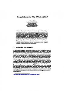
These are a generalisation of Lam´e curves (Lam´e 1818). By varying the parameters a, b, m, n1 , n2 , n3 a wide range of different shapes can be generated, often resembling shapes found in nature. In Figure 3, we depict some of the leaf-like shapes that arise from the formula by a suitable choice of parameters. Notice that with just 6 parameters we can generate many realistic leaf shapes, including fairly complex combinations of leaf base (at join with leaf stalk), overall leaf shape and leaf apex (or tip), for example reniform and cordate. This is much more expressive than simple polynomials or other general approximation methods with so few parameters. However, not all the representations of shape above are good matches to the actual meanings of the terms. For example, the entry for linear ought to be thinner and with more parallel sides. It general, the choice of parameters was guided by some general principles about the role of the individual parameters combined with a good deal of trial-and-error. The choice of parameters to generate a shape is not unique: for example, if n 2 = 0 then any value of a will suffice, likewise n 3 and b. There are more complex transformations yielding the same shape in the same position, and possibly yielding the same shape in other positions and sizes. This means that any measurement of proximity will yield zero distance between very different points in the space. That is, pseudometrics, rather than metrics, are required. Though the formula generates a wide range of shapes, this has to be balanced against its mathematical intractability. For example, whilst it is easy to get the formula to generate shapes, the inverse problem of curve-fitting, determining the parameters a, b, m, n 1 , n2 , n3 to fit a given curve, is very difficult (Osian, Tuytelaars & Gool 2004). Through experiments, we have amassed some expertise in interpreting which parameters to change at a point in the space in order to effect particular changes to the resulting curve. Other calculations are equally intractable. For a simplified form of the formula, the area within the curve can be expressed in terms of gamma functions (Jaklic, Leonardis & Solina 2000). However, defining important points on the curve (e.g. points of maximum width for bilaterally symmetric curves) and defining suitable metrics and paths in terms of these six parameters appears very difficult. With such a mechanism for describing a wide variety of leaf shapes, it may be imagined that this formula can be used to provide a semantics for leaf-shape expressions which is more expressive than the polynomial leaves described above. However, the intractability of the formula means that the constructions and transformations required to define the 20

linear

oblong

rhombic

lanceolate

ovate

elliptic

obovate

cuneate

spatulate

oblanceolate

orbicular

reniform

cordate

deltoid

hastate

sagittate

Figure 3: Some generated leaf-like shapes. Shapes are oriented so that the base is at the bottom of each image. See text for commentary. semantics are difficult to discover and difficult to express satisfactorily. Even the simple transformations of [[broadly]] and [[narrowly]] are difficult to define accurately – the way that the parameters need to be transformed varies considerably with leaf shape in an apparently rather unsystematic way. For this reason, an expressive formula as above is not, as it stands, an appropriate model for leaf-shape semantics. Can we rescue the situation? That is, can we use the simplicity and expressiveness of the formula for generating shapes, but another mechanism for defining the semantic operations? The clue to this lies in the attempt to define a (pseudo)metric on the parameter space. What is an appropriate pseudometric? Clearly not any of the standard metrics on R6 , as the parameters have very different roles in the formula. What is required is a pseudometric which reflects proximity and distance of shapes and not of parameters. This is both a geometric question and, to some extent, a botanical question. Namely, what attributes of leaf shape determine the similarity of, and distance between, shapes, and how do we rank these attributes? For complex shapes this is a difficult determination and really does require botanical input to decide on the important factors and those which, because of natural variation, are less important in determining proximity. For simple leaf shapes, such as those depicted above, we may devise a series of attributes which contribute to semantic distance. An example of such a series is: (1) (2) (3) (4)

width to length ratio, position along length of widest part, apex angle, and angle at base with petiole (leaf stalk).

These attributes may be combined into a pseudometric as a product in various ways, the most obvious is a Euclidean pseudometric, in which we may introduce weights to 21

correspond to the importance of the attribute in leaf shape determination. For Gielis’ formula, expressing these attributes as simple closed expressions appears not to be possible and so we have to resort to numerical methods to extract these factors from each shape. To define the semantic operations we combine explicit transformations with the generative power of the formula. Thus a shape is generated as an instance of the formula followed by a transformation. Suitable (pseudo)metrics, generated by a series of attributes, such as the series above, can be defined on these spaces. With such a pseudometric, we may define regions of the space for the denotation of basic terms much as we did for the case of polynomials above. The constructions and transformations corresponding to semantic operations are then defined by their effect on these attributes. For example, [[narrowly]] reduces the first attribute by a specified factor (and may change the two angles also). For leaf-shape expressions, this approach provides a tractable framework for a realistic semantics. As an example of this, we have plotted some geodesic paths through the space, using the above series of attributes of leaf shapes and an unweighted Euclidean composition as the pseudometric. In Figure 4, we illustrate a few of these paths which provide a realistic semantics for the to combination of shape expressions.

elliptic

lanceolate

obovate

lanceolate

cordate

elliptic

Figure 4: Paths among leaf shapes. In this world of leaf shapes, there is clearly much more work to do in developing models. There are many forms of leaf shape which we haven’t dealt with in the above discussion, including palmate leaves, asymmetrical leaves and leaf shapes which are not entire. Even the move to, say, lobed leaves shows that new definitions of metrics between shapes are necessary, not simply to describe more complex shapes but also to allow more complex variation of shape (e.g. a variable number of lobes). Some of the techniques of morphometric modelling with their emphasis on complex shapes and variability are particularly relevant here for developing appropriate spaces and metrics.

5.3

Analysis of real leaves

We now turn to actual leaf shapes and discuss to what extent the modelling techniques we have described capture the shape, and variation of shape, present in nature. 22

Figure 5: Leaves of Fagus sylvatica (Beech). We have sampled several species of deciduous trees, each sample taken from an area around Manchester (UK), late in the year (October/November). Larger samples covering a greater geographic area could be assembled, but the purpose at present is limited to illustrating the kind of analysis that we can perform to assess the semantics. Let us look at the results for an example species: Fagus sylvatica (Beech) with leaves variously described as: oval or obovate oval to elliptical elliptical oval ovate to elliptic. Digitized images of some Beech leaves are shown in Figure 5 to illustrate the kinds of leaf shape that these phrases are describing and also to indicate something of the variation that is present even in this small number of leaves of a single species. To assess the above semantics we have extracted numerical data from each sample. Each leaf was measured from its base (at the join of the lamina with the petiole) to the 23

Measure at quarter−way point

Measure at half−way point

Measure at three−quarter−way point

Leaf base: join with leaf−stem

Leaf length

Figure 6: Diagram of leaf measurements. end of the main lamina shape (this will not coincide with the leaf apex/tip, if this is elongated or truncated). The width of each leaf was measured at points along the length, one quarter way, half way, and three quarters way along from the base to the end of shape. See Figure 6 for a diagram depicting these measurements. We have undertaken these measurements for a sample of 30 leaves of Fagus sylvatica. A convenient view of these data is provided by the graph in Figure 7, where we plot the ratio of quarter-way width to length (marked with +) and the ratio of the three-quarterway width to the length (marked with ∗) (both along the y-axis) against the ratio of the half-way width to the length (along the x-axis). What do we observe from this plot? We now describe features of real leaves and how they are reflected in leaf descriptions: 1. Firstly, notice that, in this sample, the ratio of leaf width at the half-way point to the leaf length (the figures on the x-axis) varies from 0.54 to 0.81. Thus some leaves are almost ‘circular’ (this ratio is nearly 1) and others are longer and narrower, with a fairly even spread between these extremes. 2. Some leaves are almost symmetric about the half-way point (i.e. approach quadripartite symmetry) – these are the points where the quarter-way ratio (+) and threequarter-way ratio (*) coincide or are close and such leaves are elliptic. Those with a larger quarter-way ratio are ovate or elliptic-ovate, whilst those with a larger threequarter-way ratio are obovate or elliptic-obovate. We see that, in this sample, there is a fairly even spread between these forms of shape, with some extreme cases too. 3. We expect that as the half-way ratio increases, so do the other two measures (i.e. the leaf becomes ‘fatter’). What does this dependency look like? Both sets of data, the quarter-way ratios and the three-quarter-way ratios, approximate straight (but different) lines. The approximation to straight lines is the geodesic for the Euclidean metric in the first of the models above, saying that the proportionate increase in each of the ratios is constant when moving between shapes. How good is this approximation for this sample? In Figure 8, we plot the straight line that is the best least-squares fit using a linear regression model for the quarter-way ratio. The line has gradient 0.95, that is an increment in the half-way width is approximately matched by the same increment in the quarter-way width. 24

0.75

Ratio of width at 1/4 point (+) and at 3/4 point (*) to length

0.7

0.65

0.6

0.55

0.5

0.45

0.4

0.35

0.3 0.5

0.55

0.6 0.65 0.7 0.75 Ratio of width at half−way point to length

0.8

0.85

Figure 7: Ratios of leaf dimensions for a sample of Fagus sylvatica (Beech). The 95% confidence limits are indicated on Figure 8 as the upper and lower curves. These are almost constant at approx. 0.09 above and below the fitted line and there is a fairly uniform distribution of data points around the line. 4. Variation with size: It may have occurred to the reader that leaf shape may vary with size, even for mature leaves. An analysis of leaf-ratios to actual leaf length for this species reveals no apparent trend in the shape as the leaf gets larger. However, in some species there does appear to be a variation of shape with size. This is a form of variation which is rarely mentioned in floras, except where there is a gross difference between the shapes of smaller and larger leaves (or other causes of variation of leaf shape, e.g. species with juvenile foliage). Thus with this form of variation, descriptions might be of the form small A to large B where A and B are leaf shape expressions. This may be modelled using geodesics in product spaces. The two spaces in this example are the linear measurement of ‘size’ and the space of leaf shapes. We have undertaken a similar analysis of six other species of deciduous trees 1 . The results are broadly in agreement with that of Beech leaves – some exhibiting wider variation and others a tighter band of shapes. For details of this analysis and a review of its implication for semantics, see (Rydeheard & Wang 2006). What are the overall conclusions of this analysis of leaf shape? The results indicate that the semantics based on polynomials, including the Euclidean metric, is broadly correct for the expressions analysed and the samples measured. By extending this analysis to a wider variety of leaf shapes and measuring the attributes used in the metric, we may provide a similar assessment of models based on Gielis’ formula. Moreover, it is possible to make 1 Prunus avium (Wild cherry), Prunus spinosa (Blackthorn), Euonymus europaeus (Spindle), Nothofagus procera (Rauli), Maclura pomifera (Osage orange), and Ulmus glabra (Wych elm).

25

Ratio of breadth at quarter−way point to length

1 0.9 0.8 0.7 0.6 0.5 0.4 0.3 0.2

0.55

0.6 0.65 0.7 0.75 Ratio of breadth at half−way point to length

0.8

Figure 8: A straight line fit for leaves of Fagus sylvatica (Beech). this evaluation of models more rigorous in a variety of ways, each quantifying the degree to which semantic regions defined by authors’ descriptions of leaf shape match samples of real leaves. What is clear from this preliminary analysis is the lack of unanimity in the textual descriptions, even for this simple leaf shape, and the corresponding variation in nature. Notice that though the samples chosen are small, increasing their size can only increase variation present (though it may lead to more clustering around points or paths). For the multiple parallel descriptions, as mentioned above, a key idea is that of ‘integration’ – combining the descriptions into a single form which suitably captures the breadth of meaning without redundancy and detecting any possible inconsistency. Integration requires semantic information, and we have already begun to build automatic integration tools based on the semantic framework of this paper (see Section 8). Of course, integration itself can also be tested against nature to assess both the modelling and the integration techniques. As for the range of variation present even in this simple leaf shape, it is clear that the language for describing shape struggles not only in describing complex shapes but also in describing the complex variation present in nature.

6

Statistical analysis of text

In this section, we briefly look at another method of evaluation of models and of deriving metric information about the interpretation of phrases. Rather than compare models with nature (as above), we compare them to the texts themselves using the context and role of phrases in the texts to provide semantic information. This is necessarily a brief glimpse of the topic (which deserves a paper to itself) where, to indicate what such analysis can provide, we describe a few results of a simple experiment using a large on-line library of botanical texts. 26

Statistical analyses of large corpora of text can reveal much about how we use words, how multiple meanings and proximity of meaning are reflected by contexts, and, with collation of frequency of occurrence in contexts, there is also a predicative ability, for example, for disambiguation of words and phrases (van Rijsbergen 1979), (Landauer, Foltz & Laham 1998), (Pantel & Lin 2002), (McGreevy 1995). One question that may be addressed is to what extent do these techniques of textual analysis yield the very specific and fine-grained semantic information in a specialised domain such as botanical texts. Botanical texts differ from general corpora in several key ways: (1) they are highly structured, both in the hierarchy of classification, and within the description of each taxon, where there tends to be a uniform order of structural descriptions; (2) they use a limited and very specialised vocabulary, but mixed with phrases of a more general nature; and (3) there are many parallel descriptions of the same taxa, a fact which may provide additional semantic information. Statistical data from texts are not always easy to interpret, and with botanical texts there is a further complication, namely that frequency of occurrence is mediated not only by meaning but also by frequency in nature. Thus, for example, some combinations of leaf shape expressions may be rare not because they are far apart in meaning, but simply because few or no taxa have such combinations of leaf shape. A naive reading of frequency data would therefore set such shapes far apart, when metrically they ought to be close. Another phenomenon is that different authors may employ different naming regimes. A particular case of this is in the use of rarer names, for example trullate. Thus certain points in a semantic space may be named by one author but open to compound expressions by another. Here then, statistical analysis of a text which indicated rarity in a context would not reflect semantic distance, but merely different authors’ vocabularies. Of course, the latter may be detectable in a statistical analysis whereas the former needs botanical knowledge. With these general warnings in place, however, we will look briefly at the results of a few experiments collecting statistical data and see what the analysis can reveal. As source texts, we have used the online floras available in eFloras (www.efloras.org), taking only those in the English language. These are assembled by many authors and cover elements of floras around the world, including taxa from China, Pakistan, North America, parts of Africa, etc. We have written a small automated parsing and text extraction system to identify parts of plant descriptions and contexts for words. The texts we have used amount to 17,862 species descriptions, from which we have extracted relevant phrases and contexts. As a simple example of the analysis, in Appendix C, we display co-occurrence frequencies for a number of leaf shape terms. Some semantic information is indicated by these co-occurrences, but more detailed analyses are available which transitively link occurrence across contexts. We have undertook one such analysis of the eFloras texts using matrix decomposition methods (see (Landauer et al. 1998), (Landauer et al. 1998),(Quesada, Kintsch & Gomez 2002), (Hofmann 1999), (Pantel & Lin 2002), (B¨orner 2000)), in particular using the singular value decomposition of matrices of words against contexts followed by ‘dimension reduction’. Selecting a small group of words for leaf shape, we have used this in two ways (1) taking into account the parallel nature of botanical texts, so that each context for a word is a collection of multiple descriptions of the same species (i.e. the matrix indexes leaf-shape words against species), and (2), ignoring the parallel nature of the texts, we use the standard analysis of contexts as phrases for leaf shape description. It 27

turns out that both analyses give the same, or similar, results. For example, using 9 words for leaf shape and the eFloras texts, the similarity orders in the table below resulted. Each line here is a list of words in increasing contextual distance from the first word. linear: lanceolate ovate oblong elliptic obovate oblong: ovate lanceolate elliptic linear obovate rhombic: ovate linear lanceolate obovate oblong lanceolate: ovate oblong linear elliptic obovate ovate: lanceolate oblong elliptic linear obovate elliptic: ovate oblong lanceolate obovate linear obovate: ovate oblong lanceolate elliptic linear spathulate: oblong ovate linear lanceolate obovate oblanceolate: oblong lanceolate linear ovate elliptic We can read some metric information from these results, for instance, the proximity of narrow shapes is clearly mixed with the degree of symmetry and asymmetry (consider, for example, the occurrences of linear, lanceolate and elliptic), and the isolation of shapes such as rhombic and spatulate. Using the same analysis, we may extract clustering information indicating groups of terms with close semantic proximity. We may then compare this information with existing models, such as those in the previous section. Clearly, much more can be done in this direction, both in exploring techniques for analysing texts and also performing rigorous comparisons of the results of such analyses with the models we have constructed. Indeed, the extraction of semantic metric information from texts may contribute to the construction of metric models through a variety of techniques (for example, path metrics in graphs). Such models need to be evaluated both against nature and in terms of their utility, for example, for the automated processing of botanical texts. We intend to pursue this elsewhere, and now turn to the semantics of another continuous quantity, namely colour.

7

Colour

We now consider the semantics of expressions describing colour. Before doing so, there are several aspects of colour that need to be mentioned as they are important factors in the way that colour is generated, perceived and described. Colour arises from several different phenomena, including the presence of pigments in materials. The pigments that provide colour in plants (and more generally) are well studied and their chemical structures and absorption spectra are known. In plants, there are several families of pigments, those most important for flower colour being the anthocyanins, the flavonols, the flavones and the betalains (Salisbury & Ross 1991). Thus any colour we are describing is due to the presence of one or more of these pigments and their chemical environment. This information fixes the colour and so provides an alternative method of defining plant colours – one that is unwieldy, generally inaccessible and far from our own perception! What we mean by a colour expression is our own perceived response to the ‘actual colour’ (i.e. the wavelengths of light). Thus one important factor in the semantics of colour is the physiology of human perception of colour. This has been extensively studied (see, for example, (Bloomer 1976)). We have three types of colour receptors with peak 28

responses (in normal illumination) in yellow-green, green and blue wavelengths. The consequence of this is that we are more sensitive to differences in shades of green than in, say, red. Different individuals respond differently to colours, at the extreme there are the colour blindnesses but more generally there can be disagreements as to whether, say, an orange is more yellow or more red, or a turquoise more green or more blue. Clearly, in describing colours in plants or other materials, the physiology of human colour perception and the variation in our responses have an important role. Through the eyes of different creatures, flowers look considerably different. For example, for insect pollinators, there are sometimes patterns called ‘pollination guides’ in the near UV, invisible to us. Birds often have four colour receptors and most mammals have, unlike ourselves, only two. It is possible to adapt the way we model colours below for other creatures. For example, the three parameter colour models we describe for human perception would be replaced with a four parameter model for birds and a two parameter model for most mammals. Whilst this has considerable biological interest, it is some way from the linguistics of colour! As mentioned before, the use of colour terms in various spoken languages has attracted a good deal of attention. The data about this usage appear to contribute to our understanding of the relationship between ‘concept’ and ‘language’, see (Byrne & Hilbert 1997) for further discussion of this aspect of linguistics. There is also a considerable body of work, more closely related to the aims of this paper, on colour naming schemes, which define colour terms in appropriate models (Berk, Brownston & Kaufman 1982b), (Berk, Brownston & Kaufman 1982a), (Conway 1992), (Mojsilovi´c 2002), (Ying Liu & Ma 2005), (Tominaga 1985), (Belpaeme 2001b), (Belpaeme 2001a), (Healey & Enns 1997), (Corridoni, Del Bimbo & Pala 1999). Some schemes simply allocate points in colour spaces to colour terms, but most attempt a reconstructive naming, allocating terms to points and hence defining regions of the colour space for each term. Such colour naming schemes are an integral part of the definition of a semantics of more general colour phrases, as we explain below. Finally, botanical texts usually use normal everyday terminology for colours, without any attempt to define the terms. In this respect, colour is very different from shape, where there is a specialist and defined terminology. (One may speculate on the reasons for this difference in treatment. Amongst the factors are the capabilities of early printing technology, and the differing roles of shape and colour in plant descriptions, the variability of colour in nature, and the lack of a good everyday nomenclature for shape.) However, alternatives are available. For example, there is the excellent Royal Horticultural Society’s Colour Chart (RHS 2005) listing 884 different colours. This is rarely used in texts for wild species, but has been adopted for describing the colour of cultivars. We have begun an experiment to use this chart to evaluate the proposed semantics of colour expressions. Colour charts for more general purposes are also available, see, for example, the ‘Pantone’ colours (www.pantone.com). The website http://tx4.us/moacolor.htm describes many colour charts and schemes.

7.1

Colour models

Let us now turn to modelling colour to provide a semantics for colour expressions. Amongst the possible models are: 1. Spectra of visible light, 29

2. Standard three-parameter colour models. These include the Red-Green-Blue (RGB) model, the Hue-Saturation-Lightness (HSL) model, the artists’ model (Red-YellowBlue), and the CIE models, amongst others (see (Foley, Dam, Feiner & Hughes 1990) for an introduction to some of these models). We deal here with (2) above, leaving light spectra to possible further study. The Red-Green-Blue (RGB) model is a simple additive model. The colours Red, Green and Blue are first fixed (the criteria for this depend upon application). Any colour is then a combination of these three colours. Usually, each of R, G and B has a fixed range, for example 0-100, or for computer applications using 8-digit binary, 0-255. Thus, pure blue is [0,0,255], pure black is [0,0,0] and pure white is [255,255,255]. Turquoise is something like [72,209,204]. Note that this ‘primary colour’ model is not that of mixing paints which is the so-called ‘artists’ model’ (Red-Yellow-Blue). A quite different model is the Hue-Saturation-Lightness (HSL) model. This classifies colours not by contributory colour components, but by three aspects which are meant to represent better how we analyse and match colours. The three-dimensional cartesian space of RGB is replaced by the polar co-ordinates (s, h) with the hue h representing the angle around the ‘colour-wheel’, and the saturation s the distance from the centre of the wheel. Lightness is orthogonal to this and makes the colour-wheel into a double cone with apices being black (lightness is 0) and white (lightness is 1). The appropriate metric for the HSL space is the polar expression for Euclidean distance: p µ((h, s, l), (h0 , s0 , l0 )) = (l − l0 )2 + (s2 + s02 − 2ss0 cos (h − h0 )).

The second component in this expression is the distance between the two vectors (s, h) and (s0 , h0 ) in polar co-ordinates, and the first component is the Euclidean addition of the lightness. Although this is an adaptation of Euclidean distance in HSL, it translates into a non-Euclidean metric in RGB. The geodesics of this metric are indeed straight lines (not in (h, s, l) parameters, of course, but in the combination of polar and cartesian that these represent). Parameterised by t, the geodesics are: s cos (h) = αt + α0 s sin (h) = βt + β0 l = γt + γ0

where α, α0 , β, β0 , γ, γ0 are constants. Whilst the HSL model and its metric are closer to human colour perception than RGB, variant models have been proposed which are claimed to be even closer to our colour perception with metrics more exactly matching our perceived proximity of colours. For example, Sarifuddin and Missaoui (Sarifuddin & Missaoui 2005) propose a Hue-ChromaLuminance (HCL) model. The HCL model is similar to the HSL model in that hue is represented as an angle on the ‘colour-wheel’ and the second component, the chroma, is the distance from the origin in this disk. The luminance measures the way we respond to colour intensity, and provides an orthogonal axis making the disk into a cone. Their proposed metric is a weighted version of the HSL Euclidean metric. The CIE models are another approach to modelling colour based on human perception, the parameters of the these models are defined in terms of the colour responses of the three colour receptors in our eyes (Foley et al. 1990). 30

The three-parameter models mentioned are all equivalent in the sense that there are bijective conversions between them. However, some are closer to our visual perception and the way we separate the components of a colour. Such models are more relevant to a description of semantics. Moreover, standard metrics in some models do not reflect the semantics of colour, for example, the Euclidean metric in the the RGB model does not correctly capture perceived colour differences (Sarifuddin & Missaoui 2005).

7.2

Semantics of colour

We now explore the possibility of using these models to give a semantics of colour expressions as they occur in botany. As an example, we use the HSL model and its metric – it being a standard model reflecting, to some extent, our visual perception. Basic colour terms are interpreted in this model using one of the colour naming schemes referenced above for allocating regions to words such as red, blue etc. and for colour modifiers pale, deep etc. An appropriate scheme for this semantics is (Mojsilovi´c 2002) which describes, for basic colour terms, regions of the HSL space. We extend this to a semantics of colour phrases using the metric semantics described in Section 4. With these two ingredients we can interpret general colour phrases as regions of the HSL space, using its Euclidean metric to determine proximity and paths. To compare the semantics with actual colours in nature, we adopt a simple strategy. We use digital images of flower colours and analyse them to find the position of the colour components of pixels in the colour model. As mentioned previously, there is a good deal of processing and transformation of colour in these images from the original reflected light to the image processed for colour information, and indeed the camera itself is adapted to our own colour responses. However, we intend this not as a definitive evaluation but as an indication of evaluation methods for the semantics and the sorts of results we may expect. Let’s begin with simple colour words as they are used in botany. In Figure 9, we depict the pixel colours of three blue flowers in the Hue-Saturation-Lightness model. The image is a projection of the HSL double cone onto its ‘base’, i.e. depicts only the variation of Hue with Saturation. The saturation varies from zero at the centre to maximum at the perimeter. The flowers analysed are (1) Centaurea cyanus (Cornflower) whose major pigment is Protocyanin (Shiono, Matsugaki & Takeda 2005) and whose flower colour is variously described as: blue violet-blue or dark blue, rarely white or purple violet-blue, outer dark blue, white or purple usually blue, sometimes pink or white blue, and (2) Myosotis ramosissima (Early Forget-me-not), variously described as: mid-blue bright blue blue (rarely white), and finally (3) Commelina diffusa (Climbing Dayflower), which is described as:

31

red

yellow

magenta

Centaurea cyanus

Myosotis ramosissima green

blue Commelina diffusa

cyan

Figure 9: HSL plot of pixel colours of various blue flowers. upper petals blue bright blue, or rarely white medium blue blue. What is clear from the colour plot is that the colours of the flowers occupy different regions of the HSL space, all near blue. Some of the authors quoted have attempted to describe more precisely these regions, either by saying which colour areas to move towards to modify pure blue (e.g. violet-blue) or with modifiers such as mid, medium, bright or dark. Notice also that the degree of saturation is fairly low, and varies between species, with Cornflower having a greater saturation (maximizing at approx. 60%) – a fact which is less apparent from the botanical descriptions. Let us now turn to descriptions of colour variation. As an example of a plant whose flowers exhibit a range of colours, consider Pulmonaria longifolia (Narrow-leaved Lungwort). This is described as: more vivid blue [than P. officinalis] red at first, soon turning to violet or violet-blue violet to violet-blue blue to violet when open. Notice that the color range is here mixed with flower maturity in a product metric. In Figure 10, we depict the flower colour in HSL for flowers of differing ages. The first plot is the the projection of the double cone onto its base, i.e. the variation of Hue with Saturation, displayed as in the previous plot. The second plot is the projection of the HSL double cone on the red-cyan axis, with red on the right. As expected, the plots display a much greater range of colours than is evident in the blue flowers previously discussed. 32

white red

yellow

magenta

violet

green

blue

black

cyan

Figure 10: HSL plots of the flower colour pixels for Pulmonaria longifolia. The first plot shows that the hues are indeed in a range from fairly pure blue through to red (on the blue side of reds) and the second plot shows that the red pixels (on the right) are predominantly in the darkish red area (the bottom centre is the lower apex of the cone and is black, the top centre being white), whilst the blue pixels (on the left) range more widely, especially in the lighter blues where they extend out to a saturation of nearly 60%. Several things are not apparent from these plots. For example, how frequent are the reds and the blues, and is the frequency fairly even between these or does it peak? In Figure 11, we plot the frequencies of pixels against the hue, with the x-axis denoting the percentage distance around the colour wheel. We notice that the distribution is bimodal, with two peaks, one in the blue (the first narrower peak at c68), and one in purplish red area (the second broader peak at c90) and a marked dearth of pixels of intermediate hue. This corresponds to the observation that these flowers are initially purplish red when opening, but then rapidly progress through intermediate colours to stabilise around the blue peak. The colour-ranges in the descriptions of Pulmonaria longifolia are interpreted by the semantics as straight-line geodesics in this model. It is clear that a broader spread of colours is present than would be expected from a direct reading of the semantics. There are several reasons for this. Firstly, there is the paucity of our standard vocabulary for colours and colour ranges, and our meagre use of precision in everyday descriptions of colour, and the concentration of this description on the hue component. Thus botanists are unlikely to attempt to capture the real variation present in these plots, even if they chose to do so. In this, we are in a similar situation to leaf shapes, as we are with the multiplicity of different parallel colour descriptions, and the possibility of integration using the semantics. Moreover, it is not clear how much the ranges in the plots are artifices of the colour processing in digital images. Of course, this doesn’t preclude our trying to describe these ranges, but they may not exactly match what a botanist is seeing. To reach a conclusion here, other techniques are necessary. We have begun to use the RHS colour chart (RHS 2005) as a means of allocating flower colours to points in the HSL space and compare these with the semantics. Initial results have been encouraging in their degree of support for this semantic modelling. 33

250

Frequecies of pixels

200

150

100

50

0

0

20

40

60 Hue

80

100

120

Figure 11: Plot of frequency against hue for the colour pixels of Pulmonaria longifolia. This is clearly only the beginning of an analysis of the semantics of colour expressions in botany. The techniques described above suggest a series of further experiments in this practical approach to semantics.

8

Applications: Information retrieval and integration

Semantics has a fundamental role in the automated processing of text, in information extraction, in database ontologies and in description logics for database interrogation, where the logical aspects of querying are combined with models of the relevant structures, including models of continuous quantities as we present in this paper. With such a semantics, we may address questions such as: how do we detect inconsistency in knowledge bases, especially, in the applications to botany, inconsistency in multiple parallel descriptions? Moreover, a semantics is necessary for proper data integration: combining the information in parallel descriptions without redundancy and with due regard for the range of variation amongst descriptions. A metric semantics allows us to identify and compare regions of space so that consistency can be described in terms of proximity and integration is the assembling of descriptions of compound regions. When incorporated into ontologies and description logics, such semantic tools can provide powerful mechanisms for the organisation, processing and exploration of knowledge bases. For this to be effective, the semantics needs to be in a suitable computational form and the incorporation of this into a description logic should extend the automated reasoning ability without a significant deterioration in its performance. An ontology-based approach to extracting and collating parallel information from multiple botanical textual sources and storing it in a suitable electronic form is described in (Lydon et al. 2003), (Wood et al. 2004), (Wood & Wang 2004) and (Wood et al. 2003). This work however does not support a semantics of the descriptive phrases which form a key component of such texts. In more recent work, Wang and Pan (Wang & Pan 2005) have incorporated into this ontology the semantic modelling described in this present 34

paper and shown how it may be combined with a description logic reasoner (FaCTDG see (Bechhofer, van Harmelen, Hendler, Horrocks, McGuinness, Patel-Schneider & (eds.) 2004) and (Pan 2004)). The process of incorporating semantic information into ontologies and description logics begins by representing phrases describing continuous quantities as a datatype in the description language. A subsumption relation is defined over these phrases so that more general expressions subsume more specialised expressions. Based on this subsumption relation, the description logic reasoner may then process queries of the following forms (1) exact matching, (2) subsumption, (3) specialisation (converse of subsumption), and (4) overlap (non-empty intersection). To handle integration of descriptions, explicit calculation of regions in the modelling space is required using the semantics of this paper. The metric allows us to assess the similarity of two descriptions and decide how a combined description should be formulated. This is based on an iterative process which uses simplified calculations of regions. The result of this process is not only an integrated result, but also a record of how the individual descriptions relate to the integrated result and to each other. This scheme has been implemented for colour descriptions based on the HSL model. The results of a series of experiments on botanical texts, both inferential matching and description integration, have been encouraging. We intend to use similar techniques to incorporate the semantics of shapes as described in this paper, and more generally to extend the techniques to incorporate the semantics of other continuous quantities.

9

Discussion

The purposes of this paper have been broad indeed – not only to describe a general semantic framework for continuous quantities in natural languages but also to investigate a range of models for several such quantities and to show how models may be assessed against both the physical phenomena being described and semantic information arising from textual analysis. Because of this range of issues we have been able to introduce only briefly some of these aspects and clearly much work remains to be done. Models arise from a variety of sources: (1) standard mathematical constructions of metric spaces, (2) physical phenomena (e.g. light spectra), (3) technology of devices (e.g. some of the three-parameter models of colour), (4) models of perception (e.g. other threeparameter models of colour), and (5) textual analysis of the use and context of words. Some models have a degree of ‘appropriateness’ for the role in the semantics of continuous quantities built into their construction. It is then unsurprising that these models are adequate for the task and that the space reflects a semantic reality which we can compare with the physical phenomena under discussion. This wealth of models and their suitability for semantics is worthy of considerably more investigation. A topic we haven’t approached yet is that of relationships between models, considering maps between models and the invariance or otherwise of the semantics under such maps. Another aspect of models under investigation is their role in computation, especially in text processing and in information structuring and retrieval. This provides further requirements on models in terms of their suitability. For the small range of models we have described, a variety of computational behaviours have been displayed. One can enumerate such computational aspects of models: for example the efficiency of computing semantic values, the computation of regions, equality, proximity and paths, and the ease 35

or difficulty of incorporating these computations into automated reasoning systems. What has become very clear during this investigation is the real variability of nature and the rather loose coupling of this with botanical description. As mentioned before, botanical descriptions are as precise as is needed for the purpose in hand (usually defining a taxon or differentiating between taxa). However, our experiments suggest an intriguing possibility, not simply ‘integrating’ different descriptions, but using the real measurements and the accompanying models to generate precise descriptions of the quantities and their variation as they occur in nature. This is a form of ‘reconstructive linguistics’ in which the ‘descriptive’ part of ‘descriptive science’ would come to the fore. It would indeed be interesting to see the phraseology needed to capture more fully nature’s variation. At the moment, we have investigated only two continuous quantities. Obviously, there are many other quantities present in botanical texts (and elsewhere). Many appear to fit fairly straightforwardly into this framework. However, interesting further issues arise in the modelling some kinds of quantities, for example temporal aspects of plant development and spatial aspects of the arrangement of plant parts. It is clear that this is just the beginning of a far more extensive investigation of the semantics of continuous quantities, leading us to consider other continuous quantities, applications other than botany, other models and further evaluation against data from nature and from texts.

Authors’ addresses Shenghui Wang, David E. Rydeheard, David S. Br´ee, School of Computer Science, The University of Manchester, Oxford Road, Manchester M13 9PL, UK. Email: [email protected], [email protected] and [email protected].

Acknowledgements We are grateful to Mary McGee Wood, who is one of the pioneers of the linguistic processing of botanical texts, in particular in the BBSRC-funded MultiFlora project. Mary has provided a focus for these activities, valuable guidance and enthusiasm, and helpful comments on this paper. We would also like to thank Elzbieta Pekalska who gladly shared her knowledge of the applications of metric spaces in computation.

Appendix A: Metric Spaces We review here the mathematics of metric spaces that we require for this presentation of semantics. For more detailed expositions see, for example, (Giles 1987) or (Copson 1968). Definition 1. A metric space (S, µ) is a set S together with a binary operation µ : S×S → R+ , where R+ is the set of non-negative real numbers, such that, for all x, y, z in S, 1. µ(x, y) = 0 ⇐⇒ x = y, 2. µ(x, y) = µ(y, x), 36

3. µ(x, z) ≤ µ(x, y) + µ(y, z). Thus µ is symmetric and satisfies the triangle inequality (the third axiom). If the weaker form of the first axiom ∀x ∈ S. µ(x, x) = 0 holds instead then we call µ a pseudometric instead of a metric. Example 1. Consider the set S = R × R, where R is the set of real numbers, and the series µi for i ≥ 1: q µi ((x1 , y1 ), (x2 , y2 )) = i (|x1 − x2 |)i + (|y1 − y2 |)i . Each µi is a metric on R × R .

For i = 1 the metric becomes µ1 ((x1 , y1 ), (x2 , y2 )) = |x1 − x2 | + |y1 − y2 | and is sometimes called the city-block metric. For i = 2, we have the familiar Euclidean metric: p µ2 ((x1 , y1 ), (x2 , y2 )) = (x1 − x2 )2 + (y1 − y2 )2 For an example of these two metrics, see Figure 12.

Example 2. Consider bounded functions integrable over an interval [a, b]. We may define several simple metrics on the space of these functions: 1. The series of metrics µi , i ≥ 0: µi (f, g) =

sZ

a

i

b

(|f (x) − g(x)|)i dx.

2. The maximum distance metric, defined as: µ(f, g) = sup({|f (x) − g(x)| : x ∈ [a, b]}). The first are the functional analogues of the metrics in Example 1. The second is the limit of the first as i tends to infinity. Functions into a pseudometric space induce a pseudometric: Given pseudometric space (S, µ) and arbitrary function f : S0 → S, we define a pseudometric on S0 as µ0 (x, y) = µ(f (x), f (y)). For µ a metric and f injective, then µ 0 is a metric. A common example of this is that any function f : X → R induces a pseudometric µ on X by µ(x, y) = |f (x) − f (y)|. Example 3. Consider undirected graphs with each edge labelled with a strictly positive real number. Each connected graph has a metric space structure given by: the points of the space are the nodes of the graph, the distance between points is the length of a shortest path between the points. 37

1 0.8

0.8

0.6

0.6

0.4

0.4

0.2

0.2

0

0

−0.2

−0.2

−0.4

−0.4

−0.6

−0.6

−0.8

−0.8

−1

−0.5

0

0.5

1

−1

−0.5

0

0.5

1

Figure 12: {(x, y) : µ((x, y), (0, 0)) = 1} for (left) the city-block metric and (right) Euclidean metric Each metric space determines a topological space: Definition 2. For metric space (S, µ), define the topological space T (S, µ) to have the set of points S. The open sets are generated from the following base: {{y ∈ S : µ(x, y) < d} : x ∈ S, d ∈ R+ } These sets are the open ‘spheres’, and the open sets O(S, µ) of the space are generated as arbitrary unions of these. A subset of S is closed if its complement is open. The same construction yields a topological space from a pseudometric. Spaces arising from metrics are Hausdorff. Notice that different metrics may yield the same topology. There are several useful types of maps between metric spaces: Definition 3. For metric spaces (S, µ) and (S 0 , µ0 ), a function f : S → S0 is 1. continuous if the function induced on the topological spaces f : T (S, µ) → T (S 0 , µ0 ) is a continuous map, 2. an isometry if ∀x, y ∈ S. µ0 (f (x), f (y)) = µ(x, y), 3. a scaling if there is a constant k ∈ R such that ∀x, y ∈ S. µ 0 (f (x), f (y)) = kµ(x, y). A bijective scaling is a similarity, 4. partially contractive if ∀x, y ∈ S. µ 0 (f (x), f (y)) 6 µ(x, y) (contractive if the inequality is strict). We now consider the notion of paths and shortest paths (sometimes called geodesics) in metric space. A path in a space (S, µ) is a continuous function u : [a, b] → S where [a, b] (a 6 b) is the closed interval of reals between a and b. Sometimes conditions stronger than continuity are imposed, but this suffices for the following definitions. Points x, y in (S, µ) are path-connected if there is a path u : [a, b] → S with u(a) = x and u(b) = y. Note that, for a pseudometric µ, all points x, y with µ(x, y) = 0 are path-connected. Shortest paths (‘geodesics’) are defined as paths parameterisable by arc-length: 38

Definition 4. A path u : [a, b] → S (with a 6 b) in a metric space (S, µ) is a shortest path or geodesic, if for all t, t0 ∈ [a, b], µ(u(t), u(t0 )) = |t − t0 |. This is a limited notion of geodesic applicable to metric spaces which have at least one such geodesic path between every pair of points. The models we consider are of this form. Geodesics may then be unique or there may be a multiplicity (sometimes an infinity) of geodesics between a pair of points. To calculate geodesic paths, often the metric space is of such a form that the length of a path can be expressed as an integral and then the shortest path is the path (in a certain set of paths) that minimizes the integral, and this can be determined by variational methods in calculus. Example 4. For the city-block metric in R n , geodesics are paths which monotonically advance towards the end-points. Thus, a continuous path u : [0, 1] → R n is a geodesic iff for all s, t ∈ [0, 1], s 6 t =⇒ u(s)i 6 u(t)i when u(0)i 6 u(1)i and u(s)i > u(t)i when u(0)i > u(1)i , where xi denotes the i-th projection, 1 6 i 6 n. For the Euclidean metric in Rn , geodesics are straight lines. We now turn to subsets of metric spaces, and introduce a notion of ‘region’ which is suitable for the purposes of the semantics: Definition 5. A region of a metric space is a subset which consists of a finite number of disjoint non-empty path-connected subsets. Other conditions on ‘regions’ may be imposed, for example they may be closed and/or bounded. What is the distance between two regions? One possible definition of such a distance is: Definition 6. The Hausdorff distance between two subsets X, Y of metric space (S, µ), is given by the expression − (X, Y ), − → µH (X, Y ) = max{← µ µ H (X, Y )} H − (X, Y ) = sup → − where ← µ H x∈X inf y∈Y (µ(x, y)) and µ H (X, Y ) = supy∈Y inf x∈X (µ(x, y)) are the directional Hausdorff distances which are defined when the sup’s and inf’s are defined. On the set of non-empty, closed, bounded subsets of S, the Hausdorff distance is defined and is a metric. Example 5. If X and Y are two spheres with radii r and s (with r > s), and distance between centres of d, then the µH (X, Y ) = d + r − s. Products of metric spaces: Metric spaces, with isometries as morphisms, do not have cartesian products. However, given metric spaces (S, µ) and (S 0 , µ0 ), we can define a pseudometric on the product of the spaces S×S 0, if we are given a function ν : R+ ×R+ → R+ , satisfying the following, for all u, v, w, x ∈ R + : ν(0, 0) = 0 ν(u + v, w + x) 6 ν(u, w) + ν(v, x) u 6 v and w 6 x =⇒ ν(u, w) 6 ν(v, x). 39

The pseudometric µ on S × S0 is defined as µ((x, x0 ), (y, y 0 )) = ν(µ(x, y), µ0 (x0 , y 0 )). If further: ν(u, v) = 0 =⇒ u = v = 0 then this pseudometric is a metric. The function ν in the above defines how the two metrics are to be composed. Examples of ν are 1. a linear combination: ν(u, v) = λ1 u + λ2 v with λ1 , λ2 > 0, 2. maximum distance: ν(u, v) = max(u, v), and √ 3. the Euclidean combination: ν(u, v) = u2 + v 2 . Products have two roles: allowing us to combine metric spaces modelling different quantities, and also in the definition of metrics for a single quantity based on a combination of separate aspects of the quantity each of which is itself a metric.

Appendix B: A glossary of some leaf-shape terms We describe a few of the commoner leaf-shape terms, including the main examples of the paper. As discussed above, there is not full agreement amongst authors on the definitions, in particular on the dimensions associated with the terms. The definitions here are based on those of the on-line glossary (Massey & Murphy 1998). See Figure 3 for pictures of a wider range of shapes. Elliptic (elliptical): A symmetric plane figure with the widest axis at the mipoint of the structure and the margins symmetrically curved. Width to length ratio in the range 1:2 to 2:3 (Stace (1997) suggests ratios in range 1:1.2 to 1:3). Lanceolate: A symmetric plane figure with the widest axis below the middle and the margins symmetrically curved. Width to length ratio in the range 1:6 to 1:3 (Stace (1997) suggests a width to length ratio of approx. 1:6). Linear: A symmetric plane figure with the widest axis at the midpoint of the structure and the margins essentially parallel. Width to length ratio less than 1:12. Oblong: A symmetric plane figure with the widest axis at the midpoint of the structure and the margins essentially parallel. Width to length ratio in the range 1:2 to 2:3 (Stace (1997) suggests ratios in range 1:1.2 to 1:3). Obovate: A symmetric plane figure with the widest axis above the middle and the margins symmetrically curved. Width to length ratio in the range 1:2 to 2:3 (Stace (1997) suggests ratios in range 1:1.2 to 1:3). Ovate (oval): A symmetric plane figure with the widest axis below the middle and the margins symmetrically curved. Width to length ratio in the range 1:2 to 2:3 (Stace (1997) suggests ratios in range 1:1.2 to 1:3). 40

Appendix C: Leaf-shape terms: co-occurrence frequencies As an example of word co-occurrence frequencies, in the table below, we tabulate some results of shape words in eFloras. The (i, i)-th entry indicates the overall number of occurrences of word i in any context. The (i, j)-th entry (for i 6= j) is the number of occurrences of the hyphenated term i-j. We have conflated some (near) synonyms in this analysis (for example, elliptical with elliptic, and circular with round and orbicular). Looking at the table, we see that lanceolate occurs overall 41685 times, in the combination lanceolate-ovate it occurs 370 times, whilst ovate-lanceolate occurs 5512 times (curiously asymmetric). subulate acicular filiform linear oblong rhombic lanceolate ovate elliptic obovate cuneate spathulate oblanceolate orbicular flabellate reniform cordate deltoid hastate sagittate pentagonal

subulate 5032 0 57 334 2 0 90 16 2 0 0 0 0 0 0 0 0 93 0 0 0

acicular 0 308 7 1 0 0 1 0 0 0 0 0 0 0 0 0 0 0 0 0 0

filiform 11 0 4040 41 3 0 2 0 0 0 0 0 0 0 0 0 0 0 0 0 0

linear 57 2 37 27080 356 1 743 22 20 21 3 131 109 3 0 0 0 50 0 0 0

oblong 0 0 0 864 41160 32 476 2606 538 1252 32 87 78 7 0 0 3 49 3 3 0

rhombic 0 0 0 4 21 3474 6 157 9 56 43 0 0 27 16 0 0 8 0 0 2

lanceolate 87 0 0 5382 3387 58 41685 5512 1367 317 0 24 1 44 0 0 5 826 5 0 0

ovate 3 0 0 23 2069 622 370 54215 898 1 2 10 8 377 3 9 189 2352 15 2 22

elliptic 2 0 0 225 1544 135 200 1862 27075 1025 2 9 18 30 0 1 0 11 0 0 0

obovate 0 0 0 30 808 195 20 10 317 17327 181 36 11 90 45 0 1 18 0 0 3

subulate acicular filiform linear oblong rhombic lanceolate ovate elliptic obovate cuneate spathulate oblanceolate orbicular flabellate reniform cordate deltoid hastate sagittate pentagonal

spathulate 0 0 0 237 216 5 19 28 27 182 27 4249 31 28 0 0 0 3 0 0 0

oblanceolate 0 0 0 400 319 7 3 15 85 107 8 54 5992 0 0 0 0 2 0 0 0

orbicular 0 0 0 2 27 52 2 875 14 214 49 14 0 36104 0 73 58 51 0 0 3

flabellate 0 0 0 0 2 5 0 2 0 8 11 0 0 6 1174 0 0 9 0 0 0

reniform 0 0 0 0 9 0 0 36 4 4 0 0 0 164 4 2730 46 53 0 0 12

cordate 0 0 0 0 17 3 0 516 8 3 0 0 0 82 0 39 10542 73 20 6 2

deltoid 54 2 0 79 75 45 118 1545 13 9 0 0 0 32 9 7 15 15794 7 2 0

hastate 0 0 0 1 14 0 6 18 1 0 0 0 0 0 0 0 11 44 627 1 0

sagittate 0 0 0 0 5 0 0 2 0 0 0 0 0 0 0 0 9 13 4 635 0

pentagonal 0 0 0 0 1 11 0 17 0 3 0 0 0 61 0 59 96 4 0 0 747

Table 1: Co-occurrence frequencies of leaf-shape terms in eFloras.

References Bechhofer, S., van Harmelen, F., Hendler, J., Horrocks, I., McGuinness, D. L., PatelSchneider, P. F. & (eds.), L. A. S. (2004), ‘OWL Web Ontology Language Reference’, http://www.w3.org/TR/owl-ref/. Belpaeme, T. (2001a), Reaching coherent color categories through communication, in ‘Kr¨ose, B. et al (eds) Proc. 13th Belgium-Netherlands Conference on Artificial Intelligence BNAIC’01’, Amsterdam, pp. 41–48. 41

Belpaeme, T. (2001b), Simulating the formation of color categories, in ‘Proceedings Int. Joint Conference on Artificial Intelligence, IJCAI’01’, pp. 393–398. Berk, T., Brownston, L. & Kaufman, A. (1982a), ‘A human factors study of color notation systems for computer graphics’, Communications of the ACM 25(8), 547–550. Berk, T., Brownston, L. & Kaufman, A. (1982b), ‘A new color-naming system for graphics languages’, IEEE Computer Graphics and Applications 2(3), 37–44. Bloomer, C. M. (1976), Principles of Visual Perception, Van Nostrand Reinhold. Bookstein, F. L. (1991), Morphometric tools for landmark data: Geometry and biology, Cambridge University Press. B¨orner, K. (2000), Extracting and visualizing semantic structures in retrieval results for browsing, in ‘ACM Digital Libraries Conference 2000’, San Antonio, Texas, pp. 234– 235. Byrne, A. & Hilbert, D. (1997), A bibliography of color and philosophy, in ‘Readings on Color, Volume 1: The Philosophy of Color’, MIT Press. Clapham, A., Tutin, T. & Warburg, E. (1973), Excursion Flora of the British Isles, Cambridge University Press. Conway, D. (1992), An experimental comparison of three natural language colour naming models, in ‘Proceedings of East-West International Conference on Human-Computer Interaction’, St. Petersburg, Russia, pp. 328–339. Copson, E. (1968), Metric Spaces, Cambridge University Press. Corridoni, J. M., Del Bimbo, A. & Pala, P. (1999), Image retrieval by color semantics, in ‘Multimedia Systems 7’, Springer-Verlag, pp. 175–183. de Bakker, J. & de Vink, E. (1996), Control Flow Semantics, MIT Press, Cambridge, MA. Dickinson, T. A., Parker, W. H. & Strauss, R. E. (1987), ‘Another approach to leaf shape comparisons’, Taxon 36(1), 1–20. Dowman, M. (2001), ‘A bayesian approach to colour term semantics’, Linguscene 1. Edelman, S. (1995), ‘Representation, similarity, and the chorus of prototypes’, Minds and Machines 5, 45–68. Egenhofer, M. & Shariff, A. R. (1998), ‘Metric details for natural-language spatial relations’, ACM Transactions on Information Systems 16(4), 295–321. Foley, J. D., Dam, A. V., Feiner, S. K. & Hughes, J. F. (1990), Computer Graphics: Principles and Practice, Addison-Wesley. G¨ardenfors, P. (2000), Conceptual Spaces: the geometry of thought, The MIT Press, Cambridge, Massachusetts. Gielis, J. (2003), ‘A generic geometric transformation that unifies a wide range of natural and abstract shapes.’, American Journal of Botany 90, 333–338. 42

Gielis, J. & Gerats, T. (2004), A botanical perspective on modeling plants and plant shapes in computer graphics, in ‘Proclamations International Conference on Computing, Communications and Control Technology’, Vol. 6, pp. 265–272. Giles, J. R. (1987), Introduction to the Analysis of Metric Spaces, Australian Mathematical Society, Lecture Series 3, Cambridge University Press. Healey, C. & Enns, J. (1997), ‘A perceptual colour segmentation algorithm’, Technical Report, University of British Columbia, Vancouver, Canada. Hofmann, T. (1999), Probabilistic latent semantic analysis, in ‘Proceedings of Uncertainty in Artificial Intelligence’, Stockholm. Jaklic, A., Leonardis, A. & Solina, F. (2000), ‘Segmentation and recovery of superquadrics’, Computational imaging and vision 20. Keet, C. M. (2003), ‘Biological data and conceptual modelling methods’, Journal of Conceptual Modeling 29. Lam´e, G. (1818), Examen des diff´erentes m´ethodes employ´ees pour r´esoudre les probl`emes de geometrie, Paris: Courcier. Lammens, J. (1994), A computational model of color perception and color naming, PhD thesis, State University of New York at Buffalo. Landauer, T. K., Foltz, P. W. & Laham, D. (1998), ‘An introduction to latent semantic analysis’, Discourse Processes 25, 259–284. Lydon, S. J., Wood, M. M., Huxley, R. & Sutton, D. (2003), ‘Data patterns in multiple botanical descriptions: implications for automatic processing of legacy data’, Systematics and Biodiversity 1, 151–157. Marchand-Maillet, S. (2006), ‘Viper’s CBIRS page’, http://viper.unige.ch/other systems. Marcus, L. F., Corti, M., Loy, A., Naylor, G. J. P. & Slice, D. E. (1996), Advances in Morphometrics, NATO Science Series A: Life Sciences v. 284, Kluwer Academic Publishers Group. Massey, J. R. & Murphy, J. C. (1998), ‘Vascular plant systematics: Categorized glossary’, http://www.ibiblio.org/botnet/glossary. McGreevy, M. (1995), ‘A relational metric, its application to domain analysis and model of a remote sensing domain’, NASA Technical Memorandum 110358, Ames Research Centre, Moffett Field, California, USA. ¨ JacobMeersman, R., Tari, Z., Hacid, M.-S., Mylopoulos, J., Pernici, B., Babaoglu, O., sen, H.-A., Loyall, J. P., Kifer, M. & Spaccapietra, S., eds (2005), On the Move to Meaningful Internet Systems 2005: CoopIS, DOA, and ODBASE, OTM Confederated International Conferences, CoopIS, DOA, and ODBASE 2005, Agia Napa, Cyprus, October 31 - November 4, 2005, Proceedings, Part II, Vol. 3761 of Lecture Notes in Computer Science, Springer.

43

Mojsilovi´c, A. (2002), A method for color naming and description of color composition in images, in ‘Proceedings of the IEEE International Conference on Image Processing, 2002’, pp. Vol. 2, 789–792. Osian, M., Tuytelaars, T. & Gool, L. V. (2004), Fitting superellipses to incomplete contours, in ‘IEEE workshop on Perceptual Organization in Computer Vision’, Washington, USA. Pan, J. Z. (2004), Description Logics: Reasoning Support for the Semantic Web, PhD thesis, School of Computer Science, The University of Manchester, Oxford Rd, Manchester M13 9PL, UK. Pantel, P. & Lin, D. (2002), Discovering word senses from text, in ‘Proceedings of 8th ACM SIGKDD Conference’, pp. 613–619. Quesada, J., Kintsch, W. & Gomez, E. (2002), A computational theory of complex problem solving using latent semantic analysis, in W. Gray & C. Schunn, eds, ‘Proceedings of the 24 th Annual Conference of the Cognitive Science Society’, Lawrence Erlbaum Associates, Mahwah, NJ, Fairfax, VA., pp. 750–755. RHS (2005), The Royal Horticultural Society Colour Chart, RHS Publications, UK. Rohlf, F. & Marcus, L. F. (1993), ‘A revolution in morphometrics’, Trends in Ecology and Evolution 8, 129–132. Rydeheard, D. E. & Wang, S. (2006), ‘The manchester computational flora website’, http://www.cs.manchester.ac.uk/flora. Salisbury, F. & Ross, C. (1991), Plant Physiology (4th edition), Brooks Cole. Sarifuddin, M. & Missaoui, R. (2005), A new perceptually uniform color space with associated color similarity measure for content–based image and video retrieval, in ‘Proc. of Multimedia Information Retrieval Workshop 2005’, Salvador Brazil. Schwering, A. (2005), Hybrid model for semantic similarity measurement, in Meersman, Tari, Hacid, Mylopoulos, Pernici, Babaoglu, Jacobsen, Loyall, Kifer & Spaccapietra (2005), pp. 1279–1295. Schwering, A. & Raubal, M. (2005), Spatial relationships for semantic similarity measurement, in ‘2nd International Workshop on Conceptual Modeling for Geographic Information Systems’, Klagenfurt, Austria. Sharon, E. & Mumford, D. (2004), 2d-shape analysis using conformal mapping, in ‘IEEE Computer Society Conference on Computer Vision and Pattern Recognition’, Vol. 2, pp. 350–357. Shiono, M., Matsugaki, N. & Takeda, K. (2005), ‘Phytochemistry: Structure of the blue cornflower pigment’, Nature 436(791). Stace, C. (1997), New Flora of the British Isles, Cambridge University Press. Stearn, W. T. (2004), Botanical Latin: history, grammar, syntax, terminology and vocabulary (4th edition), Timber Press. 44

Thompson, D. (1917), On growth and form, Cambridge University Press, London. Tominaga, S. (1985), A color-naming method for computer color vision, in ‘Proceedings 1985 IEEE Int. Conf. on Cybernetics and Society’, Tucson, Arizona, pp. 573–577. van Rijsbergen, C. J. (1979), Information Retrieval (2nd Edition), Butterworths. Veltkamp, R. C. & Hagedoorn, M. (2001), State-of-the-art in shape matching, in ‘Principles of Visual Information Retrieval, M. Lew (ed)’, Springer, pp. 87–119. Wang, S. & Pan, J. Z. (2005), Ontology-based representation and query colour descriptions from botanical documents., in Meersman et al. (2005), pp. 1279–1295. Wood, M., Lydon, S., Tablan, V., Maynard, D. & Cunningham, H. (2004), Populating a database from parallel texts using ontology-based information extraction., in F. Meziane & E. M´etais, eds, ‘Proceedings of Natural Language Processing and Information Systems, 9th International Conference on Applications of Natural Languages to Information Systems’, Springer, pp. 254–264. Wood, M. M., Lydon, S. J., Tablan, V., Maynard, D. & Cunningham, H. (2003), Using parallel texts to improve recall in IE, in ‘Proceedings of Recent Advances in Natural Language Processing (RANLP-2003)’, Borovetz, Bulgaria, pp. 505–512. Wood, M. & Wang, S. (2004), Motivation for “ontology” in parallel-text information extraction, in ‘Proceedings of ECAI-2004 Workshop on Ontology Learning and Population (ECAI-OLP), Poster’, Valencia, Spain. Ying Liu, Dengsheng Zhang, G. L. & Ma, W.-Y. (2005), Region-based image retrieval with high-level semantic color names, in ‘Proceedings 11th International Multimedia Modelling Conference MMM’05’, pp. 180–187. Zhang, Y. (2006), ‘Webpage resource on http://www.fmrib.ox.ac.uk/ yongyue/morphing.html.

45

image

morphing’,