On the solution of linear differential equations in Lie groups

Downloaded from rsta.royalsocietypublishing.org on July 23, 2014

On the solution of linear differential equations in Lie groups Phil. Trans. R. Soc. Lond. A 1999 357, doi: 10.1098/rsta.1999.0362, published 15 April 1999

Email alerting service

Receive free email alerts when new articles cite this article - sign up in the box at the top right-hand corner of the article or click here

To subscribe to Phil. Trans. R. Soc. Lond. A go to: http://rsta.royalsocietypublishing.org/subscriptions


On the solution of linear differential equations in Lie groups By A. Iserles1 a n d S. P. Nør s e t t2 1

Department of Applied Mathematics and Theoretical Physics, University of Cambridge, Silver Street, Cambridge CB3 9EW, UK 2 Institute of Mathematical Sciences, Norwegian University of Science and Technology, Trondheim, Norway The subject matter of this paper is the solution of the linear differential equation y 0 = a(t)y, y(0) = y0 , where y0 ∈ G, a(·) : R+ → g and g is a Lie algebra of the Lie group G. By building upon an earlier work of Wilhelm Magnus, we represent the solution as an infinite series whose terms are indexed by binary trees. This relationship between the infinite series and binary trees leads both to a convergence proof and to a constructive computational algorithm. This numerical method requires the evaluation of a large number of multivariate integrals, but this can be accomplished in a tractable manner by using quadrature schemes in a novel manner and by exploiting the structure of the Lie algebra. Keywords: Lie groups; differential equation; rooted trees; quadrature

1. Introduction The theme underlying this paper is the solution of the differential equation y 0 = a(t)y,

t > 0,

y(0) = y0 ∈ G,

(1.1)

+

where G is a Lie group, a : R → g is Lipschitz continuous and g is the Lie algebra of G. It is well known that the solution of (1.1) stays on G for all t > 0. The retention of this important structural feature of the differential equation under discretization is at the centre of our discussion. We briefly recall that a Lie group G is a differentiable manifold, equipped with a group structure that is continuous with respect to the underlying topology of the manifold. The Lie algebra g is the tangent space of G: the set of all possible values of γ 0 (0), where γ(t) ∈ G is a smooth curve and γ(0) = Id, the identity of G. It is a linear space closed under an binary operation [· , ·] : g × g → g. This binary operation (often termed ‘commutation’ or ‘a Lie bracket’) is linear in each component, antisymmetric: [a, b] = −[b, a],

a, b ∈ g,

and subject to the Jacobi identity [a, [b, c]] + [b, [c, a]] + [c, [a, b]] = 0.

(1.2)

A crucial feature of g is that it can be mapped to G by the exponential map: given b ∈ g and t ∈ R+ , exp(tb) ∈ G is the flow generated by the infinitesimal generator b (Olver 1995). An important special case is when G is a subgroup of either GLn (R) or GLn (C), the general linear group of all real or complex non-singular n × n matrices. It is Phil. Trans. R. Soc. Lond. A (1999) 357, 983–1019 Printed in Great Britain 983

c 1999 The Royal Society

TEX Paper


984

A. Iserles and S. P. Nørsett

then called a matrix Lie group and important special cases are: SLn (R), the special linear group of real matrices with a unit determinant; Un (C), the unitary group of complex unitary matrices; On (R), the orthogonal group of real orthogonal matrices; and the special unitary and special orthogonal groups SUn (C) = Un (C) ∩ SLn (C) and SOn (R) = On (R) ∩ SLn (R), respectively. The corresponding Lie algebras are well known (Olver 1995). In the case of matrix Lie groups, the exponential operator is just exp(tb) =

∞ X 1 (tb)k , k!

k=0

while [a, b] = ab − ba is the familiar commutator of two matrices. We assume in the sequel that G is a matrix Lie group, whereby (1.1) becomes a matricial ordinary differential system. This restriction is more in the nature of conceptualization than essence, since much of our theory (but not necessarily our computational algorithms) remains intact for general Lie groups. An important case when computation leads to additional challenges in a non-matricial case is when g consists of differential operators. This issue is outside the realm of this paper. The retention of a Lie-group structure is often an imperative in numerical discretization, since it represents invariants that are satisfied by the original differential equations. Important examples, ubiquitous in applications, include the conservation of orthogonality, volume and symplecticity (Iserles & Zanna 1996). Arguably, even more important are invariants that correspond to differential systems on homogeneous manifolds (manifolds that are invariant when subjected to a transitive group action). As long as it is known how to discretize in a Lie group, it is possible also to discretize flows on homogeneous manifolds (Munthe-Kaas 1997; Munthe-Kaas & Zanna 1997). There are two points of departure for this paper. Firstly, in an important paper, Wilhelm Magnus (1954) derived ‘the continuous analogue of the Baker–Hausdorff formula’, an expansion, Z t Z t Z κ 1 σ(t) = a(κ) dκ − a(ξ) dξ, a(κ) dκ 0

2 0

0

Z t Z κ Z

1 + 4 0

0

Z t Z

1 + 12 0

0

0 κ

ξ

a(η) dη, a(ξ) dξ, a(κ) dκ Z

a(η) dη,

0

κ

a(ξ) dξ, a(κ)

dκ + · · · ,

(1.3)

such that y(t) = exp[σ(t)]y0 ,

t > 0.

(1.4)

Magnus neither proves convergence (to quote from theorem III of Magnus (1954), ‘if certain unspecified conditions of convergence are satisfied, . . . ’), nor derives the general form of the expansion (1.3). Magnus series have received considerable attention in mathematical physics (Wilcox 1972), control theory (Brockett 1976; Sussman 1986) and the theory of differential equations (Chen 1957). Yet, their coefficients have been derived either by brute force or by a Picard-type iteration, the question of convergence has been moot and, as far as we are aware, no effort has been made Phil. Trans. R. Soc. Lond. A (1999)


On the solution of linear differential equations in Lie groups

985

to fashion Magnus series as an effective computational tool. We address ourselves to these issues in this paper, noting in passing that all the operations in (1.3) (integration, commutation and linear combination) respect the Lie algebra. Therefore, by virtue of (1.4), the solution y(t) lies in the Lie group for every t > 0. This has already been observed by Magnus. Our second point of departure is the method of Fer expansions (Fer 1958), which has been considered by the first author in a numerical setting (Iserles 1984). We let y [0] = y0 and a[0] = a and set Z t k ∞ X k [m+1] k [m] ad (t) := (−1) a (κ) dκ [a[m] (t)], m ∈ Z+ , (1.5) a (k + 1)! 0 k=1

where

( k

ad[p] [q] :=

q, k = 0, [p, ad[p]k−1 [q]], k ∈ N

(1.6)

is the adjoint operator in g. It is proved in (Iserles 1984) that a[m] (t) = O(t2 therefore y

[m]

m+1

−2

),

t → 0;

Z t Z t Z t [0] [1] [m] (t) := exp a (κ) dκ exp a (κ) dκ · · · exp a (κ) dκ y0 0

0

0

m+1

approximates the solution y of (1.1) to order 2 − 2. Judiciously truncating the expansion (1.5) and replacing integrals by quadrature formulae, this becomes the basis for an effective numerical method. Note that, according to (1.5), if a[m] lies in a Lie algebra, then so does a[m+1] . Therefore y [m+1] remains in the Lie group. It is fair to mention that the purpose of Iserles (1984) was the numerical calculation of the fundamental solution of a linear system of ordinary differential equations, and Lie groups are not even mentioned in that publication. The connection between iterated commutators and Lie-group theory was noted by Casas (1996) and Zanna (1996). It is interesting to mention the origins of the method of iterated commutators in the classical technique of Lie reduction (Zanna & Munthe-Kaas 1997). The plan of this paper is as follows. In § 2 we introduce the method of Magnus series and demonstrate that, by indexing the terms in the expansion with a subset of binary trees, it is possible to derive explicit recurrence relations, as well as a convergence proof. An implementation of Magnus series to a computational end entails an approximate quadrature of a possibly large number of multivariate integrals. This is already demonstrated by the expansion (1.3). As is well known, multivariate quadrature is computationally intensive (Cools 1997), hence presenting a major obstacle toward any numerical application of our theoretical construct. Fortunately, it is possible to reduce the cost of computation very significantly indeed by paying attention to the special form of integrands and domains of integration. As a matter of fact, the cost in function evaluations reduces to that of a single univariate quadrature! Section 3 is concerned with numerical quadrature of multivariate integrals within the context of Magnus series. Phil. Trans. R. Soc. Lond. A (1999)


986


Another important saving in a numerical implementation of Magnus series is the reduction in the number of commutators, which, in tandem with function evaluations and exponentiation, is the main contributor to the computational cost of the algorithm. The number of commutators can be overwhelmingly reduced by two devices. Firstly, subjected to our quadrature formulae, different integrals require the evaluation of the same commutators. This can be completely described by exploiting our graph-theoretical interpretation of expansion coefficients. Secondly, the Jacobi identity (1.2) allows the replacement of certain terms within quadrature formulae by linear combinations of other terms. This procedure can be quantified exactly by combinatorial theory (Onischik 1993). A helpful way to rephrase our results is by observing that our quadrature formulae project the solution into a relatively lowdimensional subspace of the Lie algebra. The reduction in the number of commutators is the theme of § 4. We have already mentioned the method of iterated commutators, which provides an alternative representation of the solution of (1.1) in a Lie group. In a sense, Magnus series and iterated commutators stand for diametrically opposed approaches: the first represents the solution as a single exponential with a ‘complicated’ argument and the second yields y(t) as an infinite product of exponentials with simple arguments. In § 5 we demonstrate that these approaches can be combined. Finally, we devote § 6 to a number of numerical examples that demonstrate that our approach works and that, indeed, it offers an avenue toward competitive computational methods. Detailed complexity analysis of different combinations of Magnus series and iterated commutators will be published elsewhere by the present authors. Section 6 is also concerned with concluding remarks and a brief discussion of the ramifications of Magnus series and of the advantages and obstacles in their numerical implementation.

2. Magnus series and binary trees We wish to represent the solution of (1.1) in the form (1.4). To this end we note the following classical theorems of Hausdorff. Although their proofs are neither new nor particularly complicated, we include them for the sake of completeness and to assist numerical analysts who might lack familiarity with this set of ideas. For simplicity’s sake, the proof of theorem 2.1 is given for the case of a matrix Lie group, whereby exp σ becomes the standard exponential function. Theorem 2.1 (Hausdorff 1906). The function σ is the solution of the differential equation ∞ X l=0

1 ad[σ]l [σ 0 ] = a, (l + 1)!

t > 0,

σ(0) = 0.

Proof . Letting (1.4) in (1.1), we deduce at once that d σ(t) −σ(t) e = a, t > 0, e dt Phil. Trans. R. Soc. Lond. A (1999)

(2.1)



987

and σ(0) = 0. But, expanding into series and changing the order of summation, X ∞ ∞ k 1 X j−1 0 k−j X (−1)l l d σ(t) −σ(t) e σ = σ σσ e dt k! j=1 l! k=1

=

∞ X l=1

l X l l X

(−1) l!

j=1 k=j

l=0

l σ j−1 σ 0 σ l−j . (−1)k k

It is trivial to prove by induction that l X l l−1 (−1)k = (−1)j , k j−1

1 6 j 6 l,

k=j

and therefore

∞ l d σ(t) −σ(t) X (−1)l X j l e = (−1) e σ j σ 0 σ l−j . dt (l + 1)! j=0 j l=0

The proof is complete since an easy induction affirms the identity l X l j l−j (−1)l−j p qp , p, q ∈ g, l ∈ Z+ . ad[p]l [q] = j j=0 Theorem 2.2 (Hausdorff 1906). Let d0 6= 0 and d(z) =

∞ X

dl z l ,

z ∈ C,

l=0

be a given function, analytic in a proper neighbourhood of the origin. Then there exists t∗ > 0 such that the solution of the equation ∞ X

dl ad[σ]l [σ 0 ] = a,

0 6 t 6 t∗ ,

σ(0) = 0,

(2.2)

l=0

is the same as that of σ0 =

∞ X

fm ad[σ]m [a],

0 6 t 6 t∗ ,

∞ X

1 , d(z)

σ(0) = 0,

(2.3)

m=0

where f (z) :=

m=0

fm z m =

z ∈ C.

Proof . Let σ be the solution of (2.3). We wish to demonstrate that it is also the solution of (2.2). It is a trivial consequence of (1.6) that ad[p]l−m [ad[p]m [q]] = ad[p]l [q], Phil. Trans. R. Soc. Lond. A (1999)

0 6 m 6 l.


988


Hence it follows by substituting σ 0 on the left-hand side of (2.2) that X ∞ ∞ ∞ X X dl ad[σ]l [σ 0 ] = dl ad[σ]l fm ad[σ]m [a] l=0

=

l=0 ∞ ∞ X X

m=0

fm dl−m ad[σ]l−m [ad[σ]m , [a]]

m=0 l=m

=

∞ X l X l=0

fm dl−m ad[σ]l [a].

m=0

Since f is the reciprocal of d, it is true that ( l X 1, l = 0, fm dl−m = 0, l ∈ N, m=0 and consequently ∞ X

dl ad[σ]l [σ 0 ] = a

l=0

and we recover (2.2).

In the case of (2.1), we have d(z) = and therefore ∞ X Bm m f (z) = z + z = 1 + 12 z + m! m=0

ez − 1 , z

1 2 12 z

−

1 4 720 z

+

6 1 30240 z

−

8 1 1209600 z

+ ··· , (2.4)

where {Bm }m∈Z+ are Bernoulli numbers (Abramowitz & Stegun 1965, p. 804). Note that B2m+1 = 0 for m ∈ N. In the sequel we address ourselves to expansions of the general equation (2.3). Whenever necessary, the coefficients {fm }m∈Z+ may be substituted in line with (2.4) but, as a rule, the more general treatment leads to a more transparent and uncluttered exposition. We note in passing that, as long as a(t) ∈ g, t > 0, it is true that σ(t) ∈ g, t > 0. Perhaps the easiest proof follows readily from (2.3) by applying the method of proof of the Picard–Lindel¨ of theorem and noting that the Lie algebra g is closed with respect to the operations of integration, commutation and linear combination. Let us examine the Magnus series (1.3). Following its inner logic, we search for a general expansion of the Lie-algebraic differential equation (2.3) in terms that are formed by multiple integrations and commutations. Let E be the set of the derivatives of all the terms in the expansion. We propose the following two composition rules, which recursively define E: (1) a(t) ∈ E; and Rt (2) if p(t), q(t) ∈ E, then [ 0 q(κ) dκ, p(t)] ∈ E. Phil. Trans. R. Soc. Lond. A (1999)



989

It is an easy exercise to verify that the first few terms in (1.3) are recovered with our two composition rules. More general analysis, however, is greatly assisted by identifying the terms in E with a subset of planar binary rooted trees. We refer to Harary (1969) for basic concepts of graph theory. We associate the function a with the trivial tree of order one, consisting of a single vertex. Moreover, given that p(t), q(t) ∈ E are associated with the planar binary trees τ1 , τ2 , respectively (a relationship that we express as p ∼ τ1 , q ∼ τ2 ), we associate τ1 Z 0

t

q(κ) dκ, p(t) ∼

τ2

s @

@s

.

In other words, we encode integration in the language of graph theory by appending a vertex to the root of a tree, whereby the new vertex becomes the root. Commutation is denoted by joining the roots of the two trees to a new vertex which, again, becomes the root. Note that the antisymmetry of the commutator implies that τ1 τ2 τ2 τ1 @ @ @s + @s = 0, while the Jacobi identity (1.2) can be recast in a graph-theoretic form as τ2 τ3 τ3 τ1 τ1 τ2 @ @ @ @s @s @s τ1 τ2 τ3 @ @ @ @s + @s + @s = 0.

(2.5)

Although of no immediate concern in this section, the Jacobi identity is critical to successful implementation of the computational procedure of this paper. Its significance will become clear in § 4. The terms in (1.3) can be associated readily with binary trees and this helps in visualizing this relationship. It is helpful, as a notational convention and in line with the definition of E, to consider σ 0 , i.e. to ‘strip’ the outer integral in each term, since this somewhat simplifies the notation. Thus,

a ∼ ω0 = s ,

s s Z t a, a ∼ ω1 = @@s 0

s

, s s @ @s

s

Z 0

t

Z a,

0

s s s @@s t a, a ∼ ω2 = @@s

s

,

Z t Z 0

0

κ

a, a , a ∼ ω3 =

s

s @ @s

s

.

Note that, while ω2 follows from a combination of ω0 with ω1 , ω3 is obtained by combining ω1 with ω0 . Anticipating notation in the sequel, we denote this in the form ω2 = R(ω0 , ω1 ), Phil. Trans. R. Soc. Lond. A (1999)

ω3 = R(ω1 , ω0 ).


990


Of course, such combinations are not commutative. In general, we seek an expansion of the form Z t ∞ X X ατ Hτ (κ) dκ, σ(t) = 0

k=1 τ ∈Tk

(2.6)

where Tk is the set of all binary trees of order k (that is, with k vertices) which corresponds to terms Hτ that can be obtained by means of our two composition rules. Thus, for example, T1 = {ω0 }, T4 = {ω1 }, T7 = {ω2 , ω3 } and Tm = ∅ for m = 2, 3, 5, 6. The coefficients ατ depend solely on the sequence {fl }l∈Z+ . As a tribute to Wilhelm Magnus, whose pioneering work (Magnus 1954) inspired our analysis, and consistently with publications that have dealt with this construct from a different point of view (cf., for example, Sussman 1986; Wilcox 1972), we henceforth call (2.6) the Magnus series of σ. Note that Hτ (t) ∈ g for all τ ∈ Tk , k ∈ Z+ , implies σ(t) ∈ g and therefore exp[σ(t)] ∈ G, provided that (2.6) converges. Let X m Z t ∞ X ατ Hτ [a], m ∈ Z+ , Um = ad k=1 τ ∈Tk

0

and therefore, according to (2.3), 0

σ =

∞ X

fm Um .

(2.7)

m=0

It follows at once from (1.6) that, for every m ∈ N, X X m−1 Z t Z t ∞ X ∞ X Um = ατ Hτ , ad ατ Hτ [a] 0

k=1 τ ∈Tk

=

X ∞ X

Z ατ

k=1 τ ∈Tk

=

∞ X X

Z

ατ

k=1 τ ∈Tk

k=1 τ ∈Tk

t

0 t

0

0

Hτ , Um−1 Hτ , Um−1 .

(2.8)

Because of the second composition rule, it follows at once by induction that for every Hτ there exist terms Hτ1 , Hτ2 , . . . , Hτr , say, such that Z Z Z Hτ := R(τ1 , τ2 , . . . , τr ) = Hτ1 , Hτ2 , . . . , Hτr , a · · · . (2.9) Proposition 2.3. For every m ∈ N it is true that Um =

∞ ∞ X X k1 =1 k2 =1

···

∞ X X X km =1 τ1 ∈T1 τ2 ∈T2

Proof . By induction on (2.8). Phil. Trans. R. Soc. Lond. A (1999)

···

X

ατ1 ατ2 · · · ατm R(τ1 , τ2 , . . . , τm ) (2.10)

τm ∈Tm



991

We denote the binary tree corresponding to R(τ1 , τ2 , . . . , τr ) by R(τ1 , τ2 , . . . , τr ). This representation is not unique, e.g. s s s s @ s @s @@s s s @@s ∼ R(ω0 , ω1 ) = R(ω2 ). To ensure uniqueness we choose τ1 , τ2 , . . . , τr as follows. Every binary tree τ that can be obtained from our composition rules can be uniquely written in the form τ [r] s τ [3] @ @s τ [2] s ·· · @ ·· @s τ [1] s s @ @s @ @s [1]

[2]

s

.

[r]

Then τ = R(τ , τ , . . . , τ ), and this is the representation that we adopt in the sequel. In particular, in the last example we obtain R(ω2 ). Proposition 2.4. Given any r ∈ N and τk ∈ Tmk , k = 1, 2, . . . , r, it is true that ord R(τ1 , τ2 , . . . , τr ) =

r X

mk + 2r + 1,

(2.11)

k=1

where ord τ is the order (i.e. the number of vertices) of the tree τ . Proof . It follows from the definition of R that ord R(τ1 , τ2 , . . . , τr ) = ord R(τ1 , τ2 , . . . , τr−1 ) + mr + 2. The proof of (2.11) follows from this identity by straightforward induction.

Corollary 2.5. Tk = ∅ whenever k 6= 1 mod 3. Proof . We prove by induction that all the trees allowed by our composition rules have order 1 mod 3. Clearly, ord ω0 = 1. Assuming that mk = 3lk + 1, k = 1, 2, . . . , r, we deduce from (2.11) that X r lk + 1 + 1. ord R(τ1 , τ2 , . . . , τr ) = 3 k=1

Hence our assertion is true.

Substitution of (2.10) in (2.7) and comparison of terms corresponding to order-k trees yields X τ ∈Tk

b(k−1)/2c

ατ Hτ =

X l=1

fl

X

X

τi ∈Ti n1 ,n2 ,...,nl ∈N n1 +···+nl =n−2l−1 i=1,2,...,l

Phil. Trans. R. Soc. Lond. A (1999)

ατ1 ατ2 · · · ατl R(τ1 , τ2 , . . . , τl )


992


for every k ∈ N. This identity simplifies by virtue of corollary 2.5 to proposition 2.4, since we need to consider only trees of order 1 mod 3: X

b3m/2c

ατ Hτ =

τ ∈T3m+1

X

X

fl

X

ατ1 ατ2 · · · ατl R(τ1 , τ2 , . . . , τl ). (2.12)

n1 ,n2 ,...,nl ∈Z+ τi ∈T3ni +1 n1 +···+nl =m−l i=1,2,...,l

l=1

Comparing the left- and right-hand sides of (2.12), we deduce that T3m+1 = {R(τ1 , τ2 , . . . , τl ) : τi ∈ T3ni +1 , i = 1, 2, . . . , l, n1 + n2 + · · · + nl + l = m, l = 1, 2, . . . , b 12 (3m)c}. (2.13) Another consequence of (2.12) is that the coefficients ατ can be evaluated recursively: αω0 = f0 , αR(τ1 ,...,τl ) = fl

l Y

ατi .

(2.14)

i=1

Table 1 displays all the expansion terms, trees and coefficients of order up to ten. Assisted by table 1, we present the first few terms of the Magnus expansion for equation (2.3): Z t Z tZ κ a(κ) dκ + f0 f1 [a(ξ), a(κ)] dξ dκ σ(t) = f0 0 0 0 Z tZ κZ κ 2 [a(η), [a(ξ), a(κ)]] dη dξ dκ + f0 f2 + f0 f12

0

0

0

0 0 tZ κZ ξ

Z tZ

+

f02 f1 f2

+

f0 f13

0

f02 f1 f2

+ f03 f3

0

Z tZ

+ f02 f1 f2 +

Z

Z

0

Z

κ

κ

0

Z

[[a(η), a(ξ)], a(κ)] dη dξ dκ

ξ

0

Z

Z η

ξ

0

[[a(ρ), [a(η), a(ξ)]], a(κ)] dρ dη dξ dκ

[[[a(ρ), a(η)], a(ξ)], a(κ)] dρ dη dξ dκ

0 0 0 tZ κZ ξZ κ

0

0

0

0

Z tZ

Z tZ 0

ξ

0

κ

0

Z

κZ

κ

Z

0

κZ

0

0

0

κ

0

η

[a(ρ), [[a(η), a(ξ)], a(κ)]] dρ dη dξ dκ [[a(ρ), a(η)], [a(ξ), a(κ)]] dρ dη dξ dκ

[a(ρ), [a(η), [a(ξ), a(κ)]]] dρ dη dξ dκ + · · · .

(2.15)

The original expansion (1.3) of Magnus (1954) is readily recovered by using the values of {fm } from (2.4). The order of magnitude of the elements in (2.4) is of interest, in particular whenever we wish to approximate y by truncating the series. Let us suppose that a(t) = O(tλ ), where λ ∈ Z+ . Insofar as the present discussion is concerned, the reader might just as well assume that λ = 0, but the more general case will be useful in § 5. We define the function βτ as the least integer such that Hτ (t) = O(tβτ ), where Hτ is an expansion term corresponding to the tree τ . Therefore: Phil. Trans. R. Soc. Lond. A (1999)


On the solution of linear differential equations in Lie groups Table 1. Expansion terms Hτ corresponding to trees τ of order 6 10, their representations G and coefficients ατ order 1

4

7

name

expression

tree

representation

coefficient

ω0

a

r

—

f0

[ a, a]

r r r @r

R(ω0 )

f0 f1

R R [ a, [ a, a]]

r r r r r @r @r

R(ω0 , ω0 )

f02 f2

R R [ [ a, a], a]

r r r @r r r @r

R(ω1 )

f0 f12

R R R [ [ a, [ a, a]], a]

r r r r r @r @r r r @r

R(ω2 )

f02 f1 f2

R R R [ [ [ a, a], a], a]

r r r @r r r @r r r @r

R(ω3 )

f0 f13

R R R [ a, [ [ a, a], a]]

r r r @r r r r r @r @r

R(ω0 , ω1 )

f02 f1 f2

R R R [ [ a, a], [ a, a]]

r r r r r r @r r @r Q Q r

R(ω1 , ω0 )

f02 f1 f2

R R R [ a, [ a, [ a, a]]]

r r r r r r @r r @r @r

R(ω0 , ω0 , ω0 )

f03 f3

ω1

ω2

ω3

10

ω4

ω5

ω6

ω7

ω8

R


993


994


(1) βω0 = λ; (2) βτ > βτ1 + βτ2 + 1, where

τ1 s @ τ = @s

(3) βτ > 2βτ1 + 2, where

τ2 ;

(2.16)

τ1 s @ τ = @s

τ2

. In other words, τ1 = τ2 in (2.16) results in a larger exponent. While (1) and (2) are trivial, the proof of (3) follows at once by letting

(2.17)

Hτ = ptβτ + O(tβτ +1 ), whereby Z

1 βτ +1 βτ +2 Hτ , Hτ = pt + O(t pt ), + O(t ) = O(t2βτ +2 ). βτ + 1 Proposition 2.6. For every τ ∈ T3k+1 , k ∈ N, it is true that βτ > (k + 1)(λ + 1). (2.18)

βτ

βτ +1

Proof . By induction. We commence by observing that, according to (3), βω1 > 2(λ + 1), consistently with (2.18). Next, suppose that τ ∈ T3k+1 , k > 2, is derived from τ1 and τ2 in line with (2.16). Then τ1 ∈ T3l+1 , τ2 ∈ T3(k−l−1)+1 for some l ∈ {0, 1, . . . , k − 1}. Note that it is impossible for both τ1 = ω0 and τ2 = ω0 . If τ2 = ω0 , then l = k − 1 and, by induction, βτ1 > (l + 1)(λ + 1). Therefore, according to (1) and (2), βτ > λ + k(λ + 1) + 1 = (k + 1)(λ + 1). An identical argument affirms (2.18) when τ1 = ω0 . Finally, if τ1 , τ2 6= ω0 , then l ∈ {1, 2, . . . , k − 2}. Hence, by induction and (2), βτ1 > (l + 1)(λ + 1), ⇒ βτ > (k + 1)(λ + 1) + 1, βτ2 > (k − l)(λ + 1), actually in excess of the lower bound (2.18). It is often possible to obtain better estimates than (2.18). Thus, for example, βω7 > 4λ + 6, because of (3), while τ1 = ω1 , τ2 = ω3 , composed with (2.16), yields k = 4 and βτ > 5λ + 6. However, the lower bound (2.18) is the best possible insofar as the totality of all the non-trivial trees is concerned. The following theorem, critical to truncating Magnus series as a means to approximate the solution of (1.1), follows at once from our analysis. Theorem 2.7. Let a(t) = O(tλ ), p ∈ N and set Z t p−1 X X σp (t) := ατ Hτ (κ) dκ. k=0 τ ∈T3k+1

0

(2.19)

Then σp (t) = σ(t) + O(t(p+1)(λ+1)+1 ); therefore exp σp (t) = y(t) + O(t(p+1)(λ+1)+1 ). Phil. Trans. R. Soc. Lond. A (1999)



995

Needless to say, as things stand, (2.15) is a purely formal construct, since we have not proved yet that a Magnus expansion converges. This is our next task. Let us assume that g is equipped with a norm k · k (as long as G is a matrix Lie group, k · k might be taken, for example, as the standard matrix Euclidean norm) and that there exist ρ, t∗ > 0 such that ka(t)k 6 ρtλ ,

0 6 t 6 t∗ .

Proposition 2.8. For every τ ∈ T3k+1 it is true that λ+1 k 2ρt . kHτ (t)k 6 ρtλ λ+1

(2.20)

Proof . By induction. The bound (2.20) is certainly true for k = 0. Suppose that k ∈ N and that τ has been obtained from τ1 ∈ T3l+1 and τ2 ∈ T3(k−l−1)+1 by means of the composition rule (2.16). Then, by the induction assumption, Z t Z t kHτ (t)k = k[ Hτ2 (κ) dκ, Hτ1 (t)]k 6 2kHτ1 (t)k kHτ2 (κ)k dκ 0

λ+1

l

λ+1

0

λ+1

ρt 2ρt 2ρt λ + 1 (k − l)(λ + 1) λ + 1 λ+1 k 2ρt 6 ρtλ , λ+1 6 2ρtλ

because l ∈ {0, 1, . . . , k − 1}.

k−l−1

Substituting (2.20) into the Magnus series, we deduce from the triangle inequality that λ+1 k+1 ∞ 2ρt 1 X θk kσ(t)k 6 2 k+1 λ+1 k=0 Z 2ρtλ+1 /(λ+1) 1 = Θ(z) dz, 0 6 t 6 t∗ , (2.21) 2 0

where θk is the number of terms in the set T3k+1 , k ∈ Z+ and Θ is the generating function of the sequence {θk }k∈Z+ : Θ(z) =

∞ X

θk z k .

k=0

Counting the members of T3k+1 is a trivial exercise in graph theory. Yet, we include it here for the sake of completeness. Every element of T3k+1 is obtained uniquely from (2.16), where τ1 ∈ T3l+1 and τ2 ∈ T3(k−l−1)+1 for some l ∈ {0, 1, . . . , k − 1}. Likewise, for every such l, τ1 and τ2 , the composition (2.16) produces an element of T3k+1 . Therefore, θk =

k−1 X l=0


θl θk−l−1 ,

k ∈ N.


996


Since θ0 = 1, we deduce that Θ(z) =

∞ X

θk z k = 1 +

k=0

∞ k−1 X X

θl θk−l−1 z k = 1 + z[Θ(z)]2 .

k=1 l=0

Therefore Θ(z) is a solution of the quadratic equation z[Θ(z)]2 − Θ(z) + 1 = 0 and analyticity at the origin implies that √ ∞ 1 − 1 − 4z X (2k)! Θ(z) = = zk . 2z k!(k + 1)!

(2.22)

k=0

We deduce not just the explicit value of θk , k ∈ Z+ , but also that Θ is analytic for all |z| 6 14 . Theorem 2.9. The Magnus series converges for all 1/(λ+1) λ+1 . 0 6 t 6 min t∗ , 8ρ Moreover, within this range of t, the solution of (1.1) obeys the inequality √ Z 8ρtλ+1 /(λ+1) 1− 1−z 1 ky(t)k 6 ky0 k exp dz . 2 0 z Proof . This follows at once from our analysis and the upper bound (2.21).

3. Numerical quadrature of multivariate integrals The first step in the implementation of a Magnus expansion as a numerical procedure is a truncation of the series. In line with theorem 2.7, if all terms corresponding to Tk , k > p are truncated, the outcome is a pth-order method (we substitute λ = 0 in (2.19)). Next, all the integrals are replaced by quadratures of a sufficiently high order and, finally, we need to evaluate an exponential of an element in the Lie algebra g. On the face of it, the most computationally expensive step is the replacement of integrals by quadrature formulae†. Multivariate numerical integration is typically very expensive (Cools 1997) and we need to approximate a significant number of integrals, e.g. four integrals for order p = 4 and nine for order p = 5. Naively, each integral might be approximated by Gaussian quadrature optimized with respect to the (multivariate) domain of integration; for example, Z h ν1 X a(κ) dκ = h bj a(cj h), Z 0

hZ 0

0

κ

[a(ξ), a(κ)] dξ dκ =

j=1 ν2 X ˜bj [a(˜ h2 cj,1 h), a(˜ cj,2 h)], j=1

where {cj : j = 1, 2, . . . , ν1 } are Gaussian points in [0, 1], {(˜ cj,1 , c˜j,2 : j = 1, 2, . . . , ν2 } are Gaussian points in the triangle with vertices at {(0, 0), (1, 0), (0, 1)}, while bj and † We do not address ourselves in this paper to the evaluation of the exponential function. Phil. Trans. R. Soc. Lond. A (1999)



997

˜bj are appropriate weights. In that case, stipulating that both quadratures are of the same order of accuracy requires ν2 = O(ν12 ). Further integrals, across polyhedra of increasingly higher dimension, require even more function evaluations. Fortunately, the naive approach is completely unnecessary and, as we demonstrate in this section, the evaluation of all the necessary quadratures to order p can be accomplished in just b 12 (p + 1)c function evaluations. Given τ ∈ T3m+1 , we can write the integral of Hτ in the form Z h Hτ (t) dt I(h) := 0

Z =

h

Z

κi0

Z

0

0

0

κi1

Z ···

κim−1

0

L(a(κ0 ), a(κ1 ), . . . , a(κm )) dκm dκm−1 · · · dκ0 , (3.1)

where ij ∈ {0, 1, . . . , j},

j = 0, 1, . . . , m − 1

and m+1 times

z }| { L : g × g × ··· × g → g is a multilinear form. For example, (2.15) demonstrates that τ τ τ τ

= ω0 = ω1 = ω2 = ω3

: : : :

L(x0 ) = x0 , L(x0 , x1 ) = [x1 , x0 ], i0 = 0, L(x0 , x1 , x2 ) = [x2 , [x1 , x0 ]], i0 = 0, L(x0 , x1 , x2 ) = [[x2 , x1 ], x0 ], i0 = 0,

i1 = 0, i1 = 1.

Let c1 , c2 , . . . , cν be ν distinct points in the interval [0, 1], where ν ∈ N is given. We wish to approximate Z h Hτ (t) dt 0

by the quadrature formula I(h) ≈ Q(h) := hm+1

X

bl L(a(cl0 h), a(cl1 h), . . . , a(clm h)),

(3.2)

l∈Λν m

where Λνm is the set of all the combinations l = (l0 , l1 , . . . , lm ) of (m + 1)-tuples of integers from the set {1, 2, . . . , ν} and the weights bl are given. Note that the implementation of (3.2) requires the evaluation of the function a at just ν points. Moreover, as long as we can use the same nodes c = (c1 , c2 , . . . , cν ) for all the integrals, the entire evaluation of σp requires just ν function evaluations! Let uj ∈ Pν−1 be the jth cardinal polynomial of Lagrange interpolation at the points c1 , c2 , . . . , cν , ν Y t − ci uj (t) = , c − ci i=1 j i6=j


j = 1, 2, . . . , ν.


998


We approximate a by its Lagrange interpolation polynomial ν X t , a(cj h)uj a(t) ≈ a ˆ(t) = h j=1 hence a ˆ(ck h) = a(ck h), k = 1, 2, . . . , ν, and define the weights bl through the explicit formula Z 1 Z κi0 Z κi1 Z κi ν m−1 Y bl = ··· uli (κi ) dκm dκm−1 · · · dκ0 , l ∈ Λνm . (3.3) 0

0

0

0

i=1

Because of the multilinearity of L, we have ˆ(κ1 ), . . . , a ˆ(κm )) L(ˆ a(κ0 ), a X ν ν ν X X κ0 κ1 κm =L a(cl0 h), a(cl1 h), . . . , a(clm h) u l0 u l1 u lm h h h l0 =1 l1 =1 lm =1 ν ν ν X ν Y X X κi L(a(cl0 h), a(cl1 h), . . . , a(clm h)). ··· u li = h i=0 l0 =1 l1 =1

lm =1

Therefore, with the above definition of bl , Z h Z κi0 Z κi1 Z κi m−1 Q(h) = ··· L(ˆ a(κ0 ), a ˆ(κ1 ), . . . , a ˆ(κm )) dκm dκm−1 · · · dκ0 . 0

0

0

0

(3.4)

The identity (3.4) provides both the raison d’etre for the definition (3.3) and a convenient means for an order analysis of the quadrature formula Q(h). Let S = Si := {(κ0 , κ1 , . . . , κm ) ∈ Rm+1 : 0 6 κj 6 κij−1 , j = 1, 2, . . . , m}, so that hS is the domain of integration in (3.1), and dκ = dκm dκm−1 · · · dκ0 , therefore

Z I(h) =

ZhS

Q(h) =

hS

L(a(κ0 ), a(κ1 ), . . . , a(κm )) dκ, L(ˆ a(κ0 ), a ˆ(κ1 ), . . . , a ˆ(κm )) dκ.

Given that a(t) =

∞ X

ak tk+λ ,

k=0

where λ ∈ Z+ , and letting Lk := L(ak0 , ak1 , . . . , akm ), Phil. Trans. R. Soc. Lond. A (1999)



999

we thus deduce that Z X ∞ ∞ ∞ X X I(h) = ··· Lk κk00 +λ κk10 +λ · · · κkmm +λ dκ hS k =0 k =0 0 1 (m+1)(λ+1)

=h

= h(m+1)(λ+1)

km =0

∞ ∞ X X

···

k0 =0 k1 =0 ∞ ∞ X X

···

k0 =0 k1 =0

where

Z γk =

S

∞ X km =0 ∞ X

h

k0 +k1 +···+km

Z Lk

S

κk00 +λ κk10 +λ · · · κkmm +λ dκ

hk0 +k1 +···+km γk Lk ,

km =0

κk00 +λ κk10 +λ · · · κkmm +λ dκ,

k ∈ (Z+ )m+1 .

(3.5)

Likewise, it follows from (3.2) that Q(h) = hm+1

X

∞ ∞ X X

bl

l∈Λν m

= h(m+1)(λ+1)

···

k0 =0 k1 =0 ∞ X

∞ X

···

k0 =0 k1 =0

where δk =

X l∈Λν m

∞ X km =0 ∞ X

Lk ckl00 +λ ckl11 +λ · · · cklmm +λ hk0 +k1 +···+km +(m+1)λ

hk0 +k1 +···+km δk Lk ,

km =0

bl ckl00 +λ ckl11 +λ · · · cklmm +λ ,

k ∈ (Z+ )m+1 .

(3.6)

Comparing (3.5) with (3.6), we deduce the following order condition for the quadrature formula. Proposition 3.1. The quadrature method (3.2) is of order p ∈ N, i.e. Q(h) = I(h) + O(hp+1 ) for all sufficiently smooth functions a, if and only if δk = γk ,

k ∈ (Z+ )m+1 ,

k0 + k1 + · · · + km 6 p − (m + 1)(λ + 1).

(3.7)

Letting pj (t) :=

ν X i=1

ui (t)cji ,

j ∈ Z+ ,

we can simplify (3.6) by substituting the definition (3.3) of bl . The outcome is Z δk = pk0 +λ (κ0 )pk1 +λ (κ1 ) · · · pkm +λ (κm ) dκ, k ∈ (Z+ )m+1 . (3.8) S

It follows at once from the properties of Lagrange cardinal polynomials, ui , that pj (t) = tj + ω(t)ej (t),

j ∈ Z+ ,

where ω(t) :=

ν Y k=1


(t − ck )

(3.9)


1000


and ej ∈ Pj−ν , the set of polynomials of degree j − ν. (We let Pj−ν = {0} for j < ν.) Substituting (3.9) into (3.8), we obtain Z Y m k +λ [κj j + ω(κj )ekj +λ (κj )] dκ. (3.10) δk = S j=0

Altogether, we have 2m+1 terms in the integrand. One of these, namely κk00 +λ κk11 +λ · · · κkmm +λ , is precisely the integrand in (3.5). We wish to explore the conditions that ensure that all the remaining 2m+1 − 1 terms vanish. Given such a term, F (κ0 , κ1 , . . . , κm ), say, there exists an index r ∈ {0, 1, . . . , m} such that k

r−1 F (κ0 , κ1 , . . . , κm ) = κk00 +λ κk11 +λ · · · κr−1

+λ

ω(κr )ekr +λ (κr ) · · · .

Suppose that r > 1. In that case we execute (r − 1) exchanges of the order of integration so that κr is the last to be integrated. We commence by exchanging the order of κr and κr−1 . The outcome is Z 1 Z κi0 Z κi Z χr Z κir Z κi Z κi r−3 r−2 m−1 ··· ··· F (κ0 , κ1 , . . . , κm ) 0

0

0

0

ψr

0

0

× dκm · · · dκr+1 dκr−1 dκr dκr−2 · · · dκ0 , where

( (ψr , χr ) =

(κr , κir−2 ), (0, κir−1 ),

ir−1 = r − 1, ir−1 ∈ {0, 1, . . . , r − 2}.

Continuing in this manner, we arrive at Z χm Z 1 Z χ1 Z χ2 ··· F (κ0 , κ1 , . . . , κm ) dκm · · · dκr+1 dκr−1 · · · dκ0 dκr , 0

ψ1

ψ2

where

ψm

( ψj , χj ∈

{0, κr , κ0 , κ1 , . . . , κj−2 }, j = 1, 2, . . . , r {0, κ0 , κ1 , . . . , κj−1 , 1}, j = r + 1, . . . , m.

Relabelling the variables, we deduce that Z 1 Z Z F (κ0 , κ1 , . . . , κm ) dκ = ω(κ0 )ekr +λ (κ0 ) K(κ1 , κ2 , . . . , κm ) dκ, S

A

0

where A = {(κ1 , κ2 , . . . , κm ) ∈ Rm : ψj 6 κj 6 χj , j = 1, 2, . . . , m}, ψj ∈ {0, κ0 , κ1 , . . . , κj−1 }, j = 1, 2, . . . , m, χj ∈ {κ0 , κ1 , . . . , κj−1 , 1}, and K(κ1 , κ2 , . . . , κm ) =

m Y j=1


p˜j (κj ).

(3.11)



1001

Each p˜j (t) in the above definition is either ω(t)elj +λ (t) or tlj +λ , where ( kj−1 , j = 1, 2, . . . , r, lj = kj , j = r + 1, . . . , m. For example, Z 1 Z κ0 Z κ1 Z 0

0

0

κ1

κk00 +λ κk11 +λ κk22 +λ ω(κ3 )ek3 +λ (κ3 ) dκ3 dκ2 dκ1 dκ0 0 Z 1 Z 1 Z κ1 Z κ2 = ω(κ0 )ek3 +λ (κ0 ) κk10 +λ κk21 +λ κk32 +λ dκ3 dκ2 dκ1 dκ0 , 0

κ0

κ0

0

and hence (ψ1 , χ1 ) = (κ0 , 1),

(ψ2 , χ2 ) = (κ0 , κ1 ),

(ψ3 , χ3 ) = (0, κ2 )

and p˜j (t) = tkj +λ ,

j = 1, 2, 3.

Each p˜j is a polynomial of degree lj + λ. Therefore, and bearing in mind the definition of (ψi , χi ), i = 1, 2, . . . , m, it follows at once by induction that p˜m (κm ) ∈ Plm +λ [κm ] Z χm ⇒ p˜m (κm ) dκm ∈ Plm +λ1 [κ0 , . . . , κm−1 ] ψm Z χm−1 Z χm ⇒ p˜m−1 (κm−1 )˜ pm (κm ) dκm dκm−1 ∈ Plm−1 +lm +2(λ+1) [κ0 , . . . , κm−2 ] ψm−1

ψm

⇒ ··· Z χ1 Z χm ⇒ ··· p˜1 (κ1 ) · · · p˜m (κm ) dκm · · · dκ1 ∈ Pl1 +···+lm +m(λ+1) [κ0 ] ψ1 ψm Z ⇒ K(κ1 , . . . , κm )dκm · · · dκ1 ∈ Pl1 +···+lm +m(λ+1) [κ0 ]. A

Since l1 + · · · + lm = k0 + · · · + kr−1 + kr+1 + · · · + km and ekr +λ ∈ Pkr +λ−ν , it follows from (3.11) that Z 1 Z F (κ0 , κ1 , . . . , κm ) dκ = ω(κ)q(κ) dκ, (3.12) S

0

where q ∈ Pk0 +k1 +···+km +(m+1)(λ+1)−ν−1 . Theorem 3.2. Let us suppose that the polynomial ω obeys the orthogonality conditions Z 1 ω(κ)κj−1 dκ = 0, j = 1, 2, . . . , r. (3.13) 0

Then Q(h) is an order-(ν + r) approximation to the multivariate integral I(h). Phil. Trans. R. Soc. Lond. A (1999)


1002


Proof . Subject to (3.13), it follows from (3.12) that k0 + k1 + · · · + km 6 r + ν − (m + 1)(λ + 1) implies Z F (κ0 , κ1 , . . . , κm ) dκ = 0. S

This is true with regard to all the 2m+1 − 1 terms in the integrand. In other words, just one term contributes to the integral (3.10) and we deduce that γk = δk . The theorem now follows from the order condition (3.7). Corollary 3.3. Let (c1 , c2 , . . . , cν ) be the nodes of Gaussian quadrature in [0, 1]. Then Q(h) is a quadrature of order 2ν. To rephrase theorem 3.2 and corollary 3.3, the underlying order conditions are nothing else but the usual orthogonality conditions that guarantee the order of a univariate quadrature. All the necessary integrals can thus be evaluated to order p by evaluating the function a at just b 12 (p + 1)c Gauss–Legendre points in [0, 1] or, for that matter, at b 12 pc + 1 Gauss–Radau points there. As a trivial example, we choose λ = 0, ν = 2 and the Gauss–Legendre points √ √ c1 = 12 − 16 3, c2 = 12 + 16 3. Therefore, √ √ u1 (t) = 12 − (t − 12 ) 3, u2 (t) = 12 + (t − 12 ) 3. Brief calculation affirms that the fourth-order quadrature is Z hZ κ 1 √ 1 √ 3)L1,2 + ( 18 + 12 3)L2,1 + 18 L2,2 ]. L(a(κ), a(ξ)) dξ dκ ≈ h2 [ 18 L1,1 + ( 18 − 12 0

0

In the special case when L(x, y) = [y, x], which is of concern in this paper, obvious cancellations yield Z hZ κ √ [a(ξ), a(κ)] dξ dκ ≈ 16 3h2 [a(c1 h), a(c2 h)]. 0

0

Likewise, Z h Z h Z Hω2 (κ) dκ = 0 3

h 0

κ

a(ρ) dρ, a(ξ) dξ, a(κ) dκ 0 3 1 √ + 16 3)[[a(c1 h), a(c2 h)], a(c1 h)] ≈ h {−( 80 3 1 √ + ( 80 − 16 3)[[a(c1 h), a(c2 h)], a(c2 h)]} 3 1 √ 3 + 16 − 3)a(c1 h) − ( 80 = −h3 [[a(c1 h), a(c2 h)], ( 80

0

and Z

Z

κ

Hω3 (κ) dκ = ≈ =

0

Z h Z κ Z 0 3

ξ

1 √ 16 3)a(c2 h)]

a(ρ) dρ, a(ξ) dξ, a(κ) dκ

0 0 3 1 √ − 48 3)[a(c1 h), [a(c1 h), a(c2 h)]] h {( 80 3 1 √ − ( 80 + 48 3)[a(c2 h), [a(c1 h), a(c2 h)]]} 3 1 √ 3 1 √ − 48 + 48 3)a(c1 h) − ( 80 3)a(c2 h), [a(c1 h), a(c2 h)]]. h3 [( 80



On the solution of linear differential equations in Lie groups 1003 R R Recall, however, from (2.15) that Hω2 and Hω3 need to be evaluated as part of a linear combination. Taking this into account, we obtain Z h Z h Hω2 (κ) dκ + f0 f12 Hω3 (κ) dκ ≈ h3 [[a(c1 h), a(c2 h)], b1 a(c1 h) − b2 a(c2 h)], f02 f2 0

0

where 3 b1 = ( 80 + 3 − b2 = ( 80

2 1 √ 16 3)f0 f2 √ 2 1 16 3)f0 f2

3 + ( 80 − 3 + ( 80 +

2 1 √ 48 3)f0 f1 , √ 2 1 48 3)f0 f1 .

1 1 In particular, if f0 = 1, f1 = 12 and f2 = 12 , in line with (2.4), then b1 = b2 = 80 and Z h Z h 1 3 Hω2 (κ) dκ + f0 f12 Hω3 (κ) dκ ≈ 80 h [[a(c1 h), a(c2 h)], a(c1 h) − a(c2 h)]. f02 f2 0

0

We thus deduce from our analysis and theorem 2.7 that a fourth-order truncation of the Magnus series requires just two evaluations of a and the computation of only two commutators.

4. Reducing the number of commutators A careful reader should have observed in the last section that there is a very large scope for reducing the number of commutators that need to be evaluated to attain order 4. The number of function evaluations being determined solely by the order of the underlying method, the computation of commutators is a major expense of our algorithms, hence it makes sense to discuss in a more orderly fashion how to exploit the Lie-algebraic setting to reduce the number of commutators in a general case. Another pertinent observation from the last section is that, although a definition of the weights by the formula (3.8) makes it amenable to successful order analysis, it is not of a form suitable to a (possibly symbolic) manipulation. Recall that the terms in a Magnus expansion are indexed by binary trees and are derived naturally in terms of the composition rules from § 2. We wish to redefine the weights bl in a similar fashion. It is a tribute to the power of graph theory to illuminate the matter at hand that both goals—reduction in the number of commutators and a recursive formula for quadrature weights—can be accomplished by the same mechanism. This is the theme of the present section. Our conclusion is (we believe) striking. Recall that we need to implement the multivariate quadrature (3.2) for all trees of requisite order and that the number of such trees grows exponentially with m. Yet, as it turns out, far fewer binary trees determine the number of commutators that need be computed to attain order p. This renders our computational algorithm significantly cheaper and more competitive with alternative numerical approaches. Let τ be an arbitrary binary tree that has been constructed by the composition rules of § 2. We factorize τ into two trees, the I-tree (integration tree) and the C-tree (commutation tree) in the following manner. The I-tree is formed from τ by pruning all the vertices with two children. (By ‘pruning’ we mean a progression in a monotone ordering, from the ‘foliage’, the top of the tree, down to the root.) Similarly, the Ctree is formed by pruning all the vertices with a single child. These concepts are made considerably clearer upon an examination of an example. For instance, let us Phil. Trans. R. Soc. Lond. A (1999)


1004


consider the tree s s @@s

s

s @ @s

s s s @ s @s Z Z s

τ=

s

∈ T13 ,

which corresponds to the Magnus expansion term Z Z t Z κ0 Z κ2 Z κ3 a(κ4 ) dκ4 , a(κ3 ) dκ3 , a(κ2 ) dκ2 , 0

0

0

0

0

κ0

a(κ1 ) dκ1 , a(κ0 )

κ0 .

Our factorization yields

(I-tree) τ I = @@

and

(C-tree) τ C =

@ @ @@ Z

@ @ Z

.

For clarity, we denote the I-tree and the C-tree of τ by τ I and τ C , respectively, and use ‘ ’ and ‘ ’ to distinguish between their vertices. Every C-tree is a strictly binary tree: each vertex has either two children or none. An I-tree, however, need not be binary at all. For example, ω8I =

Z

Z .

I It is easy to verify that the R number of vertices in an I-tree τ is exactly the same as the number of integrals in Hτ . Moreover, suppose that Hτ has been derived from Hτ1 and Hτ2 by the second composition rule from § 2, i.e. that (2.16) holds. Let us define by S and Sj the polyhedra of integration in τ and in τj , j = 1, 2, respectively. Counting the number of integrals in each term, we deduce at once that

ord τ I = ord τ1I + ord τ2I . Letting m = ord τ , we set Z t Z κi1 Z Bτ,l (t) := ul0 (t) ··· 0

0

m κim−1 Y

0

and therefore, by (3.3),

l ∈ Λνm ,

i=1

Z bl =

uli (κi ) dκm dκm−1 · · · dκ1 ,

0

1

Bτ,l (t) dt.

(4.1)

Similar definitions pertain to τ1 and τ2 . It is an immediate consequence of (2.16) that Z t Z κ Bτ,l (t) = Bτ1 ,l1 (κ) Bτ2 ,l2 (ξ) dξ dκ, (4.2) 0


0



1005

where li ∈ {1, 2, . . . , ν}ord τi ,

l = (l1 , l2 ),

i = 1, 2.

The weight bl can be computed recursively by means of the formula (4.2), followed by the integral (4.1). An alternative approach is, given l ∈ Λνm , to label all the vertices of an I-tree by the cardinal Lagrange polynomials uli in a reverse natural ordering: we label the root with ul0 and then progress to label all the remaining vertices so that each child is always labelled after its parent and a child to the right is always labelled first. Thus, for example, u l4 u l3 u l2

u l 3 u l2 u l1 Z Z . u l0

u l1 @@ u l0

and

Next, the I-tree is pruned. Whenever a leaf (a childless vertex) is removed, the label of its parent is multiplied by the integral of the label of the vertex in question. Thus, for example, u l4 u l3 u l2

u l3 u l1

@@ u l0

⇒

u l2

u l2

R κ3 0

u l1 @@ u l0

R κ2 0

u l3

R κ3 0

u l4

@ @

⇒

⇒

u l4

u l1

@ u l0

ul0 (t)

Rt 0

ul2 (κ2 )

R κ2 0

ul3 (κ3 )

R κ3 0

ul4 (κ4 )

Rt 0

ul1 (κ1 )

.

The outcome, as is trivial to prove, is the polynomial Bτ,l . Finally, we use (4.1) to convert it to the weight bl . We next turn our attention to C-trees. Provided that τ ∈ T3m+1 , we deduce at once that its C-tree has order 2m + 1, since τ contains exactly m vertices with a single child. Moreover, it is trivial to observe that the C-tree has exactly m + 1 leaves (i.e. childless vertices). The C-tree determines the integrand similarly to the I-tree yielding the domain of integration. Similar connection extends to quadrature formulae (3.2): while the I-tree has just been exploited in the derivation of bl , we can use the C-tree to determine the structure of L(a(cl0 h), a(cl1 h), . . . , a(clm h)). It follows from our original definition of the connection between trees and expansion terms in the Magnus series that the Phil. Trans. R. Soc. Lond. A (1999)


1006


latter term can be obtained as follows. We label the leaves of the C-tree, progressing from the right leftwards, by a(cl0 h), a(cl1 h), . . . , a(clm h). Next we prune the tree. Each time a pair of children is pruned, their parent receives the label which is the commutator of their labels. For example, letting a[i] := a(cli h), i = 1, 2, . . . , m, a[5]

a[4]

[a[5] , a[4] ] a[3] a[2] a[1] a[3] a[2] a[1] @@ @ @ @ @ @H @ @H @ HH H ⇒ H [[a[5] , a[4] ], a[3] ] [a[2] , a[1] ] HH ⇒ H ⇒

[[[a[5] , a[4] ], a[3] ], [a[2] , a[1] ]]

.

The C-tree is instrumental not just in regard to the recovery of the exact form of commutators but also in exploiting symmetries to eliminate many of the commutators, thereby decreasing a great deal the computational expense. Recall from § 3 that Hω2 and Hω3 require the calculation of exactly the same commutators, albeit with a different labelling of the indices. This kind of symmetry is easily revealed from the structure of the C-tree. Thus, @

τωC2 =

@ @

@

@

and τωC3 = @@

.

Bearing in mind the relationship between C-trees and commutators, we observe that rotating a C-tree about a vertical axis is equivalent to exchanging the terms in the underlying commutator. In other words, a[1] @

a[2]

a[1] a[3]

@

@

a[2]

a[3] @ @ @ [1] [2] [3] [3] [1] [2] ∼ [[a , a ], a ] = −[a , [a , a ]] ∼ − @

and there is no need to evaluate the second commutator. Of course, we need to keep track of the exchange of indices, but this can be done easily. In general, we say that two strictly binary trees, τ1 and τ2 , say, are equivalent if τ2 can be converted to τ1 by a finite number of rotations with respect to vertical axes. Only a single representer from a class of equivalent trees need be evaluated for every index l. Hence, it is of interest to compare the number of equivalent trees to the overall number of strictly binary trees of any given order 2m + 1. We recall from § 2 that there are exactly θm = (2m)!/[m!(m + 1)!] members in T3m+1 , and hence this is also the number of strictly binary trees of order 2m + 1. Let θ˜m denote the number of equivalent strictly binary trees of order 2m + 1. Trivially, θ˜0 = θ˜1 = 1 and we have already seen also that θ˜2 = 1. It follows easily from table 1 that θ˜3 = 2, with Phil. Trans. R. Soc. Lond. A (1999)



1007

the representers @ @

@ @

ω4 , ω5 , ω6 , ω8 → @@

,

ω7 →

@ @ Z

@ @ Z

.

Likewise, for m = 4 we may choose the representers @ @

@@

@ @

@ @

@@

,

@@ Z Z @ @

and

@ @ Z

@ @

@ @ Z

,

and therefore θ˜4 = 3. In general, θ˜m is known in combinatorics as the mth Wedderburn–Etherington number (Comtet 1970). It is easy to affirm the recursive formula  θ˜0 = 1,     2m−2  X  1 1  θ˜2m−1 = θ˜j θ˜2m−j−2 + 2 θ˜m−1 ,  2 m ∈ N, j=0   2m−1   1 X ˜ ˜   θ˜2m = θj θ2m−j−1 ,   2 j=0

and it follows after an elementary manipulation that the generating function ˜ Θ(z) =

∞ X

θ˜m z m

m=0 2 ˜ ˜ ˜ 2 ). The asymptotic obeys the functional equation Θ(z) = 1 + 12 z[Θ(z)] + 12 z Θ(z ˜ behaviour of {θm }m∈Z+ has been determined by Otter (1948):

|θ˜m |1/m → 2.483 253 536 . . . ,

m → ∞.

This is clearly much better than the growth in the number of all rooted trees, a phenomenon illustrated in table 2. Redundancy of strictly binary trees is just one mechanism that allows us to reduce the number of commutators that need be computed. Other devices are the antisymmetry of the commutator and the Jacobi identity. We demonstrate in the sequel that an exploitation of these two devices reduces the extent of computation in the implementation of our quadrature formulae to just a single tree for every m > 0. We denote by Vm the set of all the strictly binary trees of order 2m + 1 (that is, all the C-trees that correspond to trees in T3m+1 ). Given τ ∈ Vm and a1 , a2 , . . . , am ∈ g, we say that hτ (a1 , a2 , . . . , am ) ∈ g is a realization of τ if it is obtained by the nested action of m commutators, consistently with our connection between commutation and C-trees. Thus, for example, hω2C (a1 , a2 , a3 ) = [a1 , [a2 , a3 ]] Phil. Trans. R. Soc. Lond. A (1999)

and hω7C (a1 , a2 , a3 , a4 ) = [[a1 , a2 ], [a3 , a4 ]].


1008


Table 2. The number of all C-trees (ALL) and of equivalence classes of C-trees (ECCT) for m = 0, 1, . . . , 6 m

ALL

ECCT

0 1 2 3 4 5 6

1 1 2 5 14 42 132

1 1 1 2 3 6 11

ν Let Fm stand for the linear subset of g, which is generated by all realizations [l1 ] [l2 ] hτ (a , a , . . . , a[lm ] ), where τ ranges across Vm and l ∈ Λνm . The dimension of ν is denoted by Wm,ν . Clearly, it represents the number of commutators that Rmust Fm be calculated in the implementation of the quadrature formulae (3.2) for all Hτ with τ ∈ T3m+1 . Motivated by an earlier version of this paper, Munthe-Kaas & Owren (1998) proved that in general W2,ν = 13 (ν 2 − 1)ν and W3,ν = 14 (ν 2 − 1)ν 2 †. We select a particular tree in Vm , namely

·· @ @

@@ · ··

@ @

ϕ[m] = @@ [2]

ω2C

[3]

Therefore, ϕ = and ϕ the iterated commutator,

=

ω4C .

. Each realization ϕ[m] is easily identified with

hϕ[m] (a1 , a2 , . . . , am ) = [a1 , [a2 , . . . , [am−1 , am ] · · · ]]. We adopt the notation [l1 , l2 , . . . , lm ] = hϕ[m] (a[l1 ] , a[l2 ] , . . . , a[lm ] ). ν be the linear space spanned by all the realizations of ϕ[m] . Then, according Let Km to theorem 3.1 of Onischik (1993), the Lie algebra Kν , generated by the free system of generators {a[1] , a[2] , . . . , a[ν] } can be written in the form ∞ M Kν = Krν . r=1

In particular, every term that can be generated from these elements by m commutators belongs to m M Krν . r=1

† The dimension might be reduced if there are linear dependencies between the a[j] and their comν = ∅. Moreover, needless to say, mutators. In an extreme case, if all the elements a[j] commute, then Fm it cannot exceed the dimension of g when the Lie algebra is finite dimensional. We henceforth disregard these phenomena. Phil. Trans. R. Soc. Lond. A (1999)



1009

ν We deduce that Fm is contained in the above set and conclude that m M r=1

Frν =

m M

Krν .

(4.3)

r=1

Given that Krν for r = 1, 2, . . . , m−1 would have been already evaluated, we conclude that, provided that we have calculated all the commutators corresponding to the ν , and hence all realizations of ϕ[m] in {a[0] , a[1] , . . . , a[m] }, we can compute all of Fm the quadrature formulae allowing us to advance from order m to order m + 1. This analysis affirms our observation that the realizations of ϕ[2] and ϕ[3] can be used to construct all other commutators of their orders, and it extends it to all ϕ[m] . ν is known (Onischik 1993, p. 71) and hence Moreover, the dimension of Km X 1 ν = µ(d)ν (m+1)/d , (4.4) Wm,ν = dim Km m+1 d|(m+1)

where the sum is carried out over all the divisors of m + 1 and the M¨ obius function µ(d) equals (−1)k if d is a product of k distinct primes; otherwise (i.e. when d is not square-free) it is zero (van Lint & Wilson 1992). Thus, W2,ν = 13 (ν 2 − 1)ν,

W3,ν = 14 (ν 2 − 1)ν 2 ,

W4,ν = 15 (ν 4 − 1)ν,

W5,ν = 16 (ν 3 + ν − 1)(ν 2 − 1)ν.

Unfortunately, neither (4.3) nor (4.4) is accompanied by a constructive proof that can illuminate a numerical procedure whereby the least possible number of commutators is computed. This has been recently remedied by Munthe-Kaas & Owren (1998), who have presented careful analysis and explicit algorithms that take advantage of the Jacobi identity to produce remarkable computational savings.

5. Magnus series and iterated commutators The method of Magnus series and the method of iterated commutators (Iserles 1984) represent alternative means to represent and discretize the solution of the system (1.1). Although they share the important attribute of respecting Lie-algebraic structure, the two methods are, in a sense, based on ‘orthogonal’ reasoning. While the Magnus series is based on a single exponential of an infinite (or, subject to truncation, ‘long’) expansion, the method of iterated commutators represents the solution as an infinite product of exponentials, each with a simple argument, and it approximates the solution by a finite product of this type. It is natural to consider an approach that borrows elements from both Magnus series and iterated commutators. Lemma 5.1. Let y be the solution of (1.1) and set x(t) = e−%(t) y(t),

t > 0,

where % is an arbitrary sufficiently smooth function. Then x obeys the differential equation x0 = bx, Phil. Trans. R. Soc. Lond. A (1999)

t > 0,

x(0) = Id,

(5.1 a)


1010


where b(t) =

∞ X (−1)k k=0

k!

∞ X (−1)k ad[%] [a] − ad[%]k [%0 ] (k + 1)! k

(5.1 b)

k=0

and Id is the identity. Moreover, if a, % : R+ → g then also b : R+ → g, and consequently x(t) ∈ G for every t > 0. Proof . Formally differentiating x we deduce at once that d −%(t) %(t) b(t) = e + e−%(t) a(t)e%(t) , t > 0. e dt We next replace σ with −% in the proof of theorem 2.1, concluding that k X k−m k (−1) %m ς%k−m = ad[%]k [ς], k ∈ Z+ m m=0 and

∞ X (−1)k d −%(t) %(t) e ad[%]k [%0 ]. =− e dt (k + 1)!

(5.2)

(5.3)

k=0

Employing (5.2), we also conclude that e−%(t) ae%(t) =

∞ ∞ X X (−1)k l=0 k=0

=

k!l!

%l a%k

∞ k ∞ X 1 X k l k−l X (−1)k ad[%]k [a]. (−1)l = % a% k! k! l

k=0

l=0

(5.4)

k=0

Putting (5.3) and (5.4) together, we obtain the explicit form of the function b in (5.1). The proof of the lemma is concluded by observing that both (5.3) and (5.4) produce terms in g as long as a(t), %(t) ∈ g for t > 0. Rt Note that letting %(t) = 0 a(κ) dκ results in the formula (1.5) with am ≡ a. We let a0 ≡ a and replace the Magnus expansion of σ, where y(t) = exp σ(t), with σ0,p0 ≡ σp0 , where p0 ∈ Z+ . In accordance with theorem 2.7, we note that y[0] (t) := eσ0,p0 (t) y0 = y(t) + O(tp0 +2 ).

(5.5)

Letting % ≡ σ0,p0 , we form a1 ≡ b and note that (5.5) implies that x(t) = Id +O(tp0 +2 )

and a1 (t) = O(tp0 +1 ).

Next we truncate the Magnus expansion of (5.1) as in (2.19), where p = p1 . The outcome is σ1,p1 ≡ σp1 which, after exponentiation, yields the approximant y[1] (t) = eσ0,p0 (t) eσ1,p1 (t) y0 ,

t > 0.

To examine the order of y[1] we note that theorem 2.7 need now be applied with λ = p0 + 1. Therefore, y[1] (t) = y(t) + O(t(p0 +1)(p1 +1) + 1). Phil. Trans. R. Soc. Lond. A (1999)

(5.6)


On the solution of linear differential equations in Lie groups The general pattern emerges. Given am (t) = O(tγm ), m ∈ N, where γ0 = 0, γm = (pm−1 + 1)(γm−1 + 1), m ∈ N,

1011

(5.7)

we approximate the solution of x0 = am x,

t > 0,

x(0) = Id,

by exp σx,pm . The outcome is the approximant y[m] (t) = eσ0,p0 (t) eσ1,p1 (t) · · · eσm,pm (t) y0 = y(t) + O(tγm +1 ),

t > 0.

Unless we decide to terminate, we next generate am+1 by letting a = am , % = σm,pm in (5.1). Note that (5.7) is consistent with (5.5) and (5.6). Letting pm ≡ 1 we recover the standard iterated commutators from Iserles (1984) and Zanna (1996). With greater generality, choosing pm ≡ r ∈ N, we can verify at once that γm =

r+1 [(r + 1)m − 1], r

m ∈ Z+ .

Therefore the order increases exponentially. Blending Magnus series with iterated commutators yields an abundant choice of discretization methods for every order p > 3. Each method corresponds to a specific choice of m ∈ N and p0 , p1 , . . . , pm−1 ∈ N such that γm > p. It is natural to search for a method that is, in some well-defined sense, ‘optimal’, the criterion being either the computational cost or ‘nice’ qualitative features. In a future paper we will address ourselves to complexity issues associated with different methods of this kind and demonstrate that distinct criteria of computational cost (e.g. the relative cost of commutators and of function evaluations) often lead to different optimal methods.

6. Numerical examples and concluding remarks The method of Magnus series is considerably more than just a numerical algorithm. By carrying out the full expansion or, alternatively, truncating (2.6) and subjecting the outcome to perturbation analysis, it should be possible to derive a wealth of qualitative results about linear systems (1.1). This, however, should not obscure the potential of Magnus series as a computational procedure. The main purpose of this section is to present a number of preliminary numerical results. Our goal is neither to investigate in depth the implementation of Magnus series as a numerical algorithm nor to present a compendium of comparative numerical results that might act as a guide to pros and cons of different Lie-group solvers. More modestly, we intend merely to demonstrate that the method of Magnus series, which at first glance might appear to be exotic and bizarre, can be at a relatively modest expense harnessed to produce results that display advantageous behaviour when compared with classical numerical schemes. To this end we compare three methods, all of order 4. Specializing to the linear system (1.1) and letting tn = nh, yn ≈ y(tn ), where n ∈ Z+ and h > 0 is the step-length, these methods are Phil. Trans. R. Soc. Lond. A (1999)


1012


(1) RK4. Explicit Runge–Kutta: k1 = a(tn )yn , k2 = a(tn + 12 h)(yn + 12 hk1 ),

k3 = a(tn + 12 h)(yn + 12 hk2 ), k4 = a(tn+1 )(yn + hk3 ),

yn+1 = yn + 16 h(k1 + 2k2 + 2k3 + k4 ). (2) GL4. Gauss–Legendre Runge–Kutta: √ √ k1 = a(( 12 − 16 3)h)[yn + 14 hk1 + ( 14 − 16 3)hk2 ], √ √ k2 = a(( 12 + 16 3)h)[yn + ( 14 + 16 3)hk1 + 14 hk2 ], yn+1 = yn + 12 h(k1 + k2 ).

(3) MG4. Truncated Magnus expansion with Gaussian points: √ a[1] = a(tn + ( 12 − 16 3)h), √ a[2] = a(tn + ( 12 + 16 3)h), √ 2 1 1 3 3h [a[2] , a[1] ] + 80 h [a[2] − a[1] , [a[2] , a[1] ]], σ ˜ = 12 h(a[1] + a[2] ) + 12 yn+1 = eσ˜ yn ,

with the exponential function calculated to machine accuracy by the MATLAB function expm. Note that each method requires exactly two function evaluations per step, provided that a(tn+1 ) is reused in the next step for RK4. We have applied these methods to the following three ordinary differential systems. (A) y 00 + ty = 0, y(0) = 1, y 0 (0) = 0. The equation was converted to a twodimensional vector system with 0 1 a(t) = , t > 0, −t 0 and integrated in the range 0 6 t 6 100. Note that the exact solution, a linear combination of Airy functions Ai(−t) and Bi(−t) (Abramowitz & Stegun 1965, p. 446), is asymptotically stable (Bellman 1969) and that it displays oscillations of progressively increasing frequency. Formally, conversion of the equation to a vector system yields a fundamental solution that evolves on the special linear group SL2 (R), but this is of little significance: it is the highly oscillatory behaviour of the solution that presents the most formidable computational challenge. (B) The 10 × 10 system with  2  t sin 11 kπ, k = l,   cos 2 πkt, k = l − 1, 11 k, l = 1, 2, . . . , 10, [a(t)]k,l = 2  − cos 11 πlt, k = l + 1,    0, |k − l| > 2, with y(0) = Id and 0 6 t 6 5. Note that tr a(t) = 0, and hence a(t) ∈ sl10 (R). Therefore, y lies in the special linear group, i.e. det y(t) ≡ 1. Phil. Trans. R. Soc. Lond. A (1999)


On the solution of linear differential equations in Lie groups 0.5

5

0

0

– 0.5

0

50

100

–5

0.05

0.5

0

0

0.05

0

50

100

– 0.5

1013

0

50

100

0

50

100

0

50

100

–3

5

× 10

0.05

0 –5

0

0

50

100

– 0.05

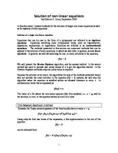
Figure 1. The error in the solution of the problem (A) by RK4 for 0 6 t 6 100. The left-hand 1 column displays the error in y, the right-hand column in y 0 , for step sizes h = 10 (top row), 1 1 h = 20 (second row) and h = 40 (bottom row).

(C) Another 10 × 10 system, namely  2  it sin 11 πk, k = l,   cos 1 πkt, k = l − 1, 5 [a(t)]k,l = 1  − cos πlt, k = l + 1,  5   0, |k − l| > 2,

k, l = 1, 2, . . . , 10,

again with y(0) = Id and 0 6 t 6 10. This time a∗ (t) + a(t) ≡ 0 and tr a(t) = 0, and therefore a(t) ∈ su10 (R): y(t) is unitary and det y(t) ≡ 1 for all t > 0. Figure 1 displays the error of RK4 for problem (A). Although the error decays consistently with order 4 when the step size h is being refined, it starts from a very substantial base. This can be attributed to the unstable and highly oscillatory nature of the exact solution of problem (A) and means that an exceedingly small step size is required for the attainment of reasonable accuracy. The implicit A-stable method GL4 is only marginally better, as is evident from figure 2. Again, the error is attenuated in line with h but, as was the case with RK4, a very small step size is required to counteract the deterioration in numerical precision. The performance of GL4 is disappointing because, according to conventional numerical wisdom, we might have expected it to perform much better than RK4 by virtue of its A-stability. Phil. Trans. R. Soc. Lond. A (1999)


1014

A. Iserles and S. P. Nørsett 0.2

2

0

0

– 0.2

0

50

100

–2

0.01

0.1

0

0

– 0.01

0

50

100

– 0.1

–4

5

50

100

0

50

100

50

100

–3

× 10

5

0

–5

0

× 10

0

0

50

100

–5

0

Figure 2. The error in the solution of the problem (A) by GL4. The interpretation of different sub-figures is the same as for figure 1.

The situation is drastically different when problem (A) is discretized with MG4, 1 , as can be ascertained from figure 3. The error for the coarsest step size, h = 10 is more than five significant digits more accurate than for the other methods! In general, it appears that the Magnus-series approach is superior, in comparison with classical methods, not just with regard to the invariance of a Lie-group structure but also in the general issue of the recovery of qualitative features and robustness with regard to ‘difficult’ phenomena like high-oscillation or complicated asymptotics. Similar pleasing behaviour is probably associated with other Lie-group methods, in particular with iterated commutators (Zanna 1996). This, we believe, is a significant observation, which should act as a spur for further research. This is perhaps the place to comment that our comparison was solely in terms of accuracy (and, in the sequel, departure from invariants) for identical step-length sequences. An alternative equally legitimate criterion is a comparison with regard to computational expense. We have not done this in general and our programs have been neither optimized for speed nor written with a variable step-size and an error controller. It might be worthwhile to mention, however, that MG4, after a minor optimization to account for the special feature of the problem (A) (in particular, with an explicit evaluation of the 2 × 2 exponential) performed significantly better (counting flops) than the MATLAB ode45 subroutine (a variable-step implementation of a fourth-order Runge–Kutta scheme). Figure 4 displays the Euclidean norm of the error in the solution of problem (B) by Phil. Trans. R. Soc. Lond. A (1999)


On the solution of linear differential equations in Lie groups –6

–6

2

× 10

1

0

–2

0

50

100

–1

1

0

50

100

× 10

–1

5

0 –1

50

100

50

100

50

100

× 10

0

–8

1

0 –8

× 10

0 –1

× 10

0

–7

1

1015

0 × 10

–10

0

0

50

100

–5

0

Figure 3. The error in the solution of the problem (A) by MG4. The interpretation of different subfigures is the same as for figures 1 and 2. 1 1 1 1 the three methods for four step-sizes, h = 10 , 20 , 50 , 100 . Note that GL4 is marginally better than RK4, while MG4, which starts similarly, accumulates error much slower than the other two methods: at t = 5 it is better roughly by a factor of 100. The exact solution of problem (B) is unstable and the extent of instability grows with increasing t. This is reflected by progressive deterioration in the absolute error for all three methods in figure 4. The main motivation for the use of a Magnus expansion is not to enhance accuracy but to force the solution to respect a Lie-group structure. Insofar as problem (B) is concerned, the Lie group is SL10 (R), hence det y(t) ≡ 1, t > 0. This is true by design (to machine accuracy) for MG4, while both RK4 and GL4 depart from the manifold. This departure is illustrated (for the same sequence of step sizes as before) in figure 5. This is perhaps the place to comment on the retention of invariants by classical numerical methods. Multistep methods score the worst and it is proved in Iserles (1997) that they retain only linear invariants. Therefore, except for the trivial case of general linear groups GLd (R) and GLd (C), they should not be used when the retention of a Lie-group structure is at issue. Certain Runge–Kutta methods—GL4, but not RK4—are somewhat better, since they can recover quadratic invariants (Calvo et al. 1996). Hence they can be safely used with the orthogonal group Od (R), the



1016


2

2

2

RK4

GL4

MG4

0

0

0

–2

–2

–2

–4

–4

–4

–6

–6

–6

–8

–8

–8

–10

– 10

– 10

0

5

0

5

0

5

Figure 4. The error log10 kyn − y(tn )k2 for the three numerical methods for problem (B) and 1 1 1 0 6 t 6 5. The solid, dot-dash, dash-dash and dotted lines correspond to h = 10 , 20 , 50 and 1 , respectively. 100

unitary group Ud (C) and the symplectic group Sp2d (R). Virtually no non-quadratic manifolds can be retained by Runge–Kutta methods (Iserles & Zanna 1999) and, in particular, no Runge–Kutta may respect manifolds that are level sets of multivariate polynomials of (total) degree greater than 3 (Iserles & Zanna 1999). Hence, no classical method is assured of retaining SLd (R) for d > 3, since the condition det y ≡ 1 for a d × d matrix y is expressible as a level set of a d-degree polynomial. Seen in this light, figure 5 is hardly surprising. Our final numerical example is problem (C) and the relevant results are displayed in figure 6. The absolute numerical error follows the same pattern as for problem (B), namely it accumulates slower with GL4 than with RK4, and yet slower with MG4. Recall that, for the present example, y(t) ∈ SU10 (C) = U10 (C) ∩ SL10 (C). In other words, y¯(t)T y(t) ≡ Id and det y(t) ≡ 1. The Magnus expansion retains, by design, both invariants, and we know that the Gauss–Legendre Runge–Kutta method GL4 retains the first and violates the second. The classical Runge–Kutta method RK4 respects neither invariant. All this is demonstrated in figure 6. We hasten to reiterate that our numerical results are not intended to present a comprehensive study, merely to provide evidence of computational potential. A future paper will address itself to detailed complexity analysis of Magnus series and of their different combinations, ´ a la § 5, with iterated commutators. Phil. Trans. R. Soc. Lond. A (1999)



1017

–3

–3 RK4

GL4

–4

–4

–5

–5

–6

–6

–7

–7

–8

–8

–9

–9

–10

–10

–11

–11 –12

–12 0

1

2

3

4

0

1

2

3

4

Figure 5. The error log10 | det yn − 1| for RK4 (left) and GL4 (right), applied to problem (B). The interpretation of different lines is the same as in figure 4.

This is the place to mention that the technique of Magnus series is not the only numerical method that is assured to stay on a Lie group. A number of alternative approaches have emerged in the past few years: the methods of rigid frames (Crouch & Grossman 1993; Owren & Marthinsen 1997), discrete gradients (Quispel & Turner 1996) and, perhaps most promisingly, Runge–Kutta methods corrected for a Lie group (Munthe-Kaas 1997). It is not the purpose of this paper to weigh the pros and cons of alternative techniques, except for observing that, in the present, nascent stateof-the-art in numerical methods on differentiable manifolds, it is perhaps premature to draw definite conclusions. To conclude this paper, we summarize its three main results. Firstly, we have formally introduced Magnus series for Lie-group linear equations (1.1) and established a relationship between their terms and a subset of binary trees. This connection is the key to the understanding and use of Magnus series, since it allows for their recursive evaluation and leads to a convergence proof. Secondly, we have demonstrated that all the integrals that are used in a discretized version of Magnus series can be approximated by using a single set of univariate quadrature points. Hence, an order-p numerical method requires just b 12 (p + 1)c function evaluations. Thirdly, using combinatorial arguments and comparing the dimension of subspaces in the Lie algebra g, we have proved that it is possible to reduce the number of commutators that are necessary to obtain an order-p discretization. Specifically, just p − 2 C-trees determine the commutators that need be evaluated, while the number of all C-trees increases exponentially with p. We believe that the approach of Magnus series is of interest both as an analytic construct and as a numerical tool. Needless to say, much remains to be done. In particular, we mention the implementation of Magnus series when a(t) is a differential operator, issues of computational complexity, generalization of the technique Phil. Trans. R. Soc. Lond. A (1999)


1018


–2

–2

–2

–4

–4

–4

–6

–6

–6

–8

–8

RK4 0

5

10

–8

GL4 0

5

10

MG4 0

5

10

0 –5 –10

RK4 0

1

2

3

4

5

6

0

7

8

9

10

0

–5

–5

– 10

– 10

RK4 0

5

10

GL4 0

5

10

Figure 6. Computational results for problem (C), 0 6 t 6 10. The top row displays the absolute 1 1 error log10 kyn − y(tn )k2 : the solid, dot-dash and dash-dash lines correspond to h = 10 , 20 and T 1 h = 50 , respectively. The middle row displays the orthogonality error log10 k¯ yn yn − Id k2 for RK4. Finally, the bottom row shows log10 | det yn − 1| for RK4 and GL4.

to nonlinear equations, and an effective approximation of the exponential which, respecting Lie groups, does not negate the most important feature of Magnus series, their retention of Lie-group structure. We hope to return to these themes in future papers. We thank Brad Baxter, Hermann Brunner, Joe Keller, Yunkang Liu, Per-Christian Moan, Robert McLachlan, Hans Munthe-Kaas, Malcolm Sabin, John Todd, Ralph Wilcox and Antonella Zanna for helpful discussions. S.P.N. was supported by the UK Engineering and Physical Sciences Research Council and by the Norwegian Research Council.

References Abramowitz, M. & Stegun, I. 1965 Handbook of mathematical functions. New York: Dover. Bellman, R. 1969 Stability theory of differential equations. New York: Dover. Brockett, R. W. 1976 Volterra series and geometric control theory. Automatica 12, 167–176. Calvo, M. P., Iserles, A. & Zanna, A. 1996 Runge–Kutta methods on manifolds. In Numerical analysis: A.R. Mitchell’s 75th birthday volume (ed. G. A. Watson & D. F. Griffiths), pp. 57– 70. Singapore: World Scientific. Casas, F. 1996 Solution of linear partial differential equations by Lie algebraic methods. Technical report, Universitat Jaume I, Spain. Phil. Trans. R. Soc. Lond. A (1999)



1019

Chen, K. T. 1957 Integration of paths, geometric invariants, and a generalized Baker–Hausdorff formula. Annals Math. 67, 164–178. Comtet, L. 1970 Analyse Combinatoire. Presses Universitaires de France. Cools, R. 1997 Constructing cubature formulas: the science behind the art. Acta Numerica 6, 1–54. Crouch, P. & Grossman, R. 1993 Numerical integration of ordinary differential equations on manifolds. J. Nonlinear Sci. 3, 1–33. Fer, F. 1958 R´esolution del l’equation matricielle U˙ = pU par produit infini d’exponentielles matricielles. Bull. Class. Sci. Acad. R. Belg. 44, 818–829. Harary, F. 1969 Graph theory. Reading, MA: Addison-Wesley. Hausdorff, F. 1906 Die symbolische Exponentialformel in der Gruppentheorie. Berichte der S¨ achsischen Akademie der Wissenschaften (Math. Phys. Klasse) 58, 19–48. Iserles, A. 1984 Solving linear ordinary differential equations by exponentials of iterated commutators. Numer. Math. 45, 183–199. Iserles, A. 1997 Numerical methods on (and off) manifolds. In Foundations of computational mathematics (ed. F. Cucker & M. Shub), pp. 180–189. New York: Springer. Iserles, A. & Zanna, A. 1996 Qualitative numerical analysis of ordinary differential equations. In The mathematics of numerical analysis (ed. J. Renegar, M. Shub & S. Smale), vol. 32 of Lectures in Applied Mathematics, pp. 421–442. Providence, RI: American Mathematical Society. Iserles, A. & Zanna, A. 1999 Numerical methods on differentiable manifolds. (In preparation.) Magnus, W. 1954 On the exponential solution of differential equations for a linear operator. Commun. Pure Appl. Math. 7, 649–673. Munthe-Kaas, H. 1997 Runge–Kutta methods on Lie groups. Technical report 122, Department of Informatics, University of Bergen. Munthe-Kaas, H. & Owren, B. 1998 Computations in a free Lie algebra. Technical report, Norwegian University of Science & Technology, Trondheim. Munthe-Kaas, H. & Zanna, A. 1997 Numerical integration of differential equations on homogeneous manifolds. In Foundations of computational mathematics (ed. F. Cucker & M. Shub), pp. 305–315. Berlin: Springer. Olver, P. 1995 Equivalence, invariants and symmetry. Cambridge University Press. Onischik, A. L. (ed.) 1993 Lie groups and Lie algebras. In Encyclopaedia of mathematical sciences, vol. 20. Berlin: Springer. Otter, R. 1948 The number of trees. Annals Math. 49, 583–599. Owren, B. & Marthinsen, A. 1997 Integration methods based on rigid frames. Technical report, Norwegian University of Science and Technology, Trondheim. Quispel, G. R. W. & Turner, G. S. 1996 Discrete gradient methods for solving ODEs numerically while preserving a first integral. Technical report, La Trobe University, Melbourne. Sussman, H. 1986 A product expansion of the Chen series. In Theory and applications of nonlinear control systems (ed. C. I. Byrnes & A. Lyndquist), pp. 323–335. New York: Elsevier. van Lint, J. H. & Wilson, R. M. 1992 A course in combinatorics. Cambridge University Press. Wilcox, R. 1972 Bounds for approximate solutions to the operator differential equation Y˙ (t) = M (t)Y (t); applications to Magnus expansions and to u ¨ + [1 + f (t)]u = 0. J. Math. Analyt. Applic. 39, 92–111. Zanna, A. 1996 The method of iterated commutators for ordinary differential equations on Lie groups. Technical Report 1996/NA12, Department of Applied Mathematics and Theoretical Physics, University of Cambridge, UK. Zanna, A. & Munthe-Kaas, H. 1997 Iterated commutators, Lie’s reduction method and ordinary differential equations on matrix Lie groups. In Foundations of computational mathematics (ed. F. Cucker & M. Shub). New York: Springer.



On the solution of linear differential equations in Lie groups

On the solution of linear differential equations in Lie groups

Suggest Documents

On the solution of linear and nonlinear partial differential equations

On the Solution of Linear Recurrence Equations

Numerical Solution of Linear Ordinary Differential Equations in ...

Lie-Groups as a Tool for Solving Differential Equations

Solving linear differential equations

LINEAR DIFFERENTIAL EQUATIONS

ON OPTIMAL SOLUTION OF INTERVAL LINEAR EQUATIONS

Solution of Systems of Linear Delay Differential Equations via Laplace

Iterative solution of differential equations

Numerical Solution of Differential Equations

Differential equations and solution of linear systems - Laboratoire Paul

Numerical Solution of Non-Linear Ordinary Differential Equations via

Analytical solution of linear ordinary differential equations by

Analytical solution of linear ordinary differential equations by ...

IRJET- Solution of Linear Differential Equations with constant Coefficients

Solution of non-linear equations

lie symmetries of differential equations by

Lie Symmetries of Differential Equations - MDPI

Symmetries of second order differential equations on Lie algebroids

DIFFERENTIAL EQUATIONS AND LINEAR ALGEBRA ...

Third Order Linear Differential Equations

Second Order Linear Differential Equations

Differential Geometry on Linear Quantum Groups

on the solution of some simple fractional differential equations