On the solution of palindromic eigenvalue problems - TU Berlin

On the solution of palindromic eigenvalue problems Andreas Hilliges‡

Christian Mehl‡

†

Volker Mehrmann‡

Abstract A rational eigenvalue problem of the form κ1 (AT1 + κA0 + κ2 A1 )x = 0 arising in the vibration analysis of rail tracks under periodic excitation is investigated. This eigenvalue problem is a special case of a more general class of problems referred to as palindromic eigenvalue problems. The paper provides the theoretical background of these eigenvalue problems and proposes a Jacobi-like algorithm for their numerical solution.

1

Introduction

In this paper, we investigate the solution of a particular rational eigenvalue problem (rational in the eigenvalue parameter) that arises in an industrial project studying the vibration of rail tracks under the excitation arising from high speed trains. This eigenvalue problem has the form 1 T (A + κA0 + κ2 A1 )y = 0, (1) κ 1 where A0 and A1 are complex n×n matrices and A0 = AT0 is complex symmetric. A matrix polynomial like the one in (1), i.e., like the matrix polynomial AT1 + κA0 + κ2 A1 , is called a palindromic matrix polynomial. This notion is based on the fact that the list (A T1 , A0 , A1 ) of coefficient matrices that is obtained by ordering the coefficient matrices with increasing powers of κ is the same as the list obtained by ordering the coefficient matrices with decreasing powers - up to transposition. The theory of palindromic matrix polynomials is discussed in detail in [3]. It is the aim of this paper to provide the theoretical background for the solution of the eigenvalue problem (1) by applying the results from [3]. The paper is organized as follows. In Section 2, we show how the eigenvalue problem (1) arises in the simulation of vibration of rail tracks under periodic excitation. In Section 3, we discuss the basic properties of palindromic matrix polynomials and show that under reasonable assumptions the problem can be linearized to a generalized eigenvalue problem that reflects the palindromic structure. This generalized eigenvalue problem is then discussed in Section 4, where also an algorithm for its numerical solution is presented. † Supported by Deutsche Forschungsgemeinschaft through DFG Research Center FZT86, ‘Mathematics for key technologies’ in Berlin. ‡ TU Berlin, Institut f¨ ur Mathematik, 10623 Berlin, Germany, e-mails: [email protected], [email protected], [email protected]

1

2

Vibration of rail tracks under periodic excitation

A project of the company SFE GmbH in Berlin investigates noise in rail traffic that is caused by high speed trains. Therefore, the vibration of an infinite rail track is simulated and analyzed for obtaining information on the development of noise between wheel and rail. In the model (see Figure 1), the rail is assumed to be infinite and is tied to the ground on sleepers, where two neighboring sleepers have a distance of s = 0.6 m (including the length of one of the sleepers). This distance is called a sleeper bay.

Figure 1: Model of the rail.

Since the structure of the rail is identical in each sleeper bay, the model will result in a periodic system as we shall see later. Using then classical finite element discretization for the model of excited vibration (see Figure 2) then leads to an infinite second order system of the form M x¨ + Dx˙ + Sx = F, with infinite block-tridiagonal symmetric coefficient matrices M, D, S, where    .  .  ... ... 0 ... 0 .. ..   ..     ...  Mj−1,0 Mj,1 0 .   Fj−1   xj−1       T Mj,1 Mj,0 Mj+1,1 0  , x =  xj  , F =  Fj M = 0    .  ...  ...  ..  T  Fj+1  xj+1  M M j+1,0 j+1,1   .. .. ... ... . . 0 ... 0

(2)



   ,  

(3)

and where D, S have the same structure as M with blocks Dj,0 , Dj,1 and Sj,0 , Sj,1 , respectively. Here, Mj,0 is symmetric positive definite and Dj,0 , Kj,0 are symmetric positive semidefinite. There are several ways to approach the solution of the problem, which presents a mixture between a differential equation (time derivatives of x) and a difference equation (space differences in j). 2

Figure 2: FE discretization of the rail in one sleeper bay.

Since one is interested in studying the behaviour of the system under excitation, the ansatz Fj = Fˆj eiωt , xj = xˆj eiωt , where ω is the excitation frequency, leads to a second order difference equation with variable coefficients for the xˆj that is given by ATj−1,j xˆj−1 + Ajj xˆj + Aj,j+1 xˆj+1 = Fˆj

(4)

with the coefficient matrices Aj,j+1 = −ω 2 Mj,1 + iωDj,1 + Kj,1 ,

Ajj = −ω 2 Mj,0 + iωDj,0 + Kj,0 .

(5)

Observing that the system matrices vary periodically due to the identical form of the rail track in each sleeper bay, we may combine the (say l) parts belonging to the rail in one sleeper bay into one vector   xˆj  xˆj+1    (6) yj =  ..  ,  .  xˆj+l

and thus obtain a constant coefficient second order difference equation AT1 yj−1 + A0 yj + A1 yj+1 = Gj 3

(7)

with coefficent matrices  Aj,j Aj,j+1 0 ... 0 ..  T ... Aj+1,j+2 .  Aj,j+1 Aj+1,j+1  . . . .. .. .. A0 =  0  0  . . .. ..  ATj+l−2,j+l−1 Aj+l−1,j+l−1 Aj+l−1,j+l 0 ... 0 ATj+l−1,j+l Aj+l,j+l

and



   A1 =   

0

0 ... ... ... ... ... ... 0 0 ...

0 .. . 0 Aj+l,j+l+1

 0 ..  .   . 0   0  0



   ,   

(8)

(9)

For this system we then make the ansatz yj+1 = κyj , which leads to the complex eigenvalue problem 1 T (A + κA0 + κ2 A1 )y = 0. κ 1

(10)

We note that A0 is complex symmetric, i.e., A0 = AT0 , and A1 is complex and singular.

3

Palindromic eigenvalue problems

The eigenvalue problem (10) is a typical example of a palindromic polynomial eigenvalue problem. A matrix polynomial P (λ) = M0 + λM1 + · · · + λk Mk

(11)

with coefficient matrices Mj ∈ Cn×n , j = 0, . . . , k is called palindromic (or, more precisely, T -palindromic, where ‘T ’ stands for ‘transpose’) if ! µ ³ ´¶T ÃX k 1 = P (λ) = λk P λk−j MjT . (12) λ j=0 Typical examples for palindromic matrix polynomials are the following: 1. P1 (λ) = M T + λM , where M ∈ Cn×n ; 2. P2 (κ) = AT1 + κA0 + κ2 A1 , where A0 , A1 ∈ Cn×n , A0 = AT0 ; 3. P3 (λ) = A + λB + λ2 B T + λ3 AT , where A, B ∈ Cn×n . 4

Using (12), one easily obtains that if λ0 6= 0 is a finite eigenvalue of a palindromic matrix polynomial P (λ), i.e., P (λ0 )x = 0 for some x ∈ Cn \ {0}, then so is 1/λ0 . Introducing homogeneous parameters, one finds similarly that also the eigenvalues zero and ∞ are paired. The theory of palindromic matrix polynomials is discussed in detail in [3]. The question arises how to solve an eigenvalue problem with underlying palindromic matrix polynomial (11). If the problem is large and sparse, then one should apply a projection method like a Jacobi-Davidson-type method (see, e.g., [5]). The basic idea of this approach is to generate a k-dimensional subspace V of Cn that contains good approximation to some of the eigenvalues of (11). Then, the projection of the original problem to this subspace is considered, i.e., one computes a matrix V ∈ Cn×k whose columns span the subspace V and then one solves the projected eigenvalue problem with underlying matrix polynomial P˜ (λ) = V T M0 V + λV T M1 V + · · · + λk V T Mk V. (13) The standard approach for solving solve its linearization   λm−1 x Am   .. I   . λ   ...   λx  x I

this small and dense eigenvalue problem would be to  λm−1 x −Am−1 . . . . . . −A0    .. I    .   = ...   λx   x I 0 





  . 

(14)

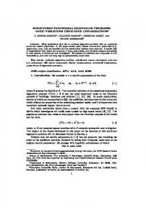
Indeed, as it is known from the theory of matrix polynomials (see [1, 2]), the eigenvalues of the matrix pencil in (14) coincide with the eigenvalues of the matrix polynomial (11). However, this linearization does not reflect the palindromic structure of the matrix polynomial. In exact arithmetic, the eigenvalues of the pencil in (14) still come in pairs (λ 0 , 1/λ0 ), but in the numerical computation, the symmetry of the spectrum might be lost due to roundoff errors. Tests show that the eigenvalues of the problem (10) vary from a magnitude of 10 −15 up to 1015 . A typical distribution of the spectrum (excluding zero and infinity) is shown in Figure 3. Here, the rail in one sleeper bay has been divided into five elements (i.e., l = 5) whereas each element has been discretized in such a way that it has 201 degrees of freedom for vibration (see Figure 2) . Thus, the matrices of the resulting eigenvalue problem (10) are of size 1005×1005. Besides zero and ∞ the spectrum of (10) consists of 134 eigenvalues which are displayed in Figure 3 ordered by magnitude. For the sake of a better visualization of the spectral symmetry, the reciprocal of the eigenvalue has been displayed rather than the eigenvalue itself whenever its modulus was smaller than one. This typical eigenvalue distribution illustrates the importance of preservation of structure in the eigenvalue computation for palindromic matrix polynomials. If non-structure preserving methods are used, it becomes very complicated to figure out which of the small and large eigenvalues are actually paired, since the small eigenvalues are completely blurred by roundoff errors. Thus, it is necessary to preserve the palindromic structure of the eigenvalue problem in each step such that the pairing of eigenvalues is automatically guaranteed. Thus, the matrix polynomial should be linearized in a palindromic way, i.e., the linearization itself should be palindromic. 5

1e+016

1e+014

1e+012

1e+010

1e+008

1e+006

10000

100

1 0

20

40

60

80

100

120

140

Figure 3: Typical eigenvalue distribution.

The question arises if it is always possible to obtain a palindromic linearization for a given palindromic matrix polynomial The answer is ‘yes up to some linearization condition’. In [3], an algorithm for a given palindromic matrix polynomial that constructs a palindromic linearization (i.e., a palindromic matrix pencil with the same spectral information) has been designed. Applying this algorithm to the particular second degree matrix polynomial in (10) leads to the following linearization: ¸ · T ¸ · A1 A0 − A 1 A1 A1 . (15) λ + AT1 AT1 A0 − AT1 A1

Thus, the problem of solving palindromic polynomial eigenvalue problems reduces to the problem of computing the eigenvalues of a matrix pencil of the form λM + M T that we will call a palindromic matrix pencil. The corresponding eigenvalue problem λM x + M T x = 0 is called the generalized palindromic eigenvalue problem.

4

The generalized palindromic eigenvalue problem

In this section, we discuss how to solve the generalized palindromic eigenvalue problem λM x + M T x, 6

(16)

where M ∈ Cn×n . This special structure is preserved by applying congruence transformations (λM + M T ) 7→ P T (λM + M T )P,

(17)

where P ∈ Cn×n is invertible. For the sake of numerical stability, we also want to choose P unitary whenever this is possible. The question arises which condensed form for the pencil in (16) should be computed. If one thinks of an analogue of the generalized Schur form and computes an upper triangular form P T M P for M , then P T M T P is lower triangular and thus, the eigenvalues cannot be read off from the diagonal of the pencil in general. However, if we compute the so-called anti-triangular form for M , i.e., if we choose P such that   0 ... 0 m1,n ..   .. . . . m2,n−1 .   . T P MP =  (18) , . ..   0 ... ... mn,1 . . . ... mn,n then also P T M T P is in anti-triangular form and one easily verifies that the eigenvalues of the pencil λM + M T are −

m1n mn1 ,...,− . m1n mn1

(19)

(Here, we assume that the pencil is regular, i.e., det λM + M T 6≡ 0, and we interprete expressions x/0, x ∈ C \ {0} as infinite eigenvalues.) The following theorem from [3] shows that this reduction is always possible, even if P is restricted to be unitary. Theorem 1 Let M ∈ Cn×n . Then there  0  ..  . T U MU =   0 mn1

exists a unitary matrix U ∈ Cn×n such that  ... 0 m1n ..  . . . m2,n−1 .  (20) . . . . ..  .. .. ... ... mnn

It should be highlighted that the matrix U in Theorem 1 is unitary, but not complex −1 orthogonal. Thus, the matrix U T M U is not similar to M , since U T = U . However, the pencils λM + M T and λU T M U + U T M T U are clearly equivalent and, therefore, have the same spectral information. From the discussion so far, we see that there is another advantage of using structure preserving, i.e., palindromic linearization. Instead of working on two matrices simultaneously (as it is usually the case with generalized eigenvalue problems), we only have to store and work on one single matrix M to obtain the full information on the spectrum of the matrix pencil λM + M T . 7

Concerning the numerical solution of the generalized palindromic eigenvalue problem (i.e., for the transformation of a matrix to anti-triangular form via a unitary congruence transformation M 7→ U T M U ), we note that currently no QR-like method is known that preserves the palindromic structure of the problem. Therefore, we suggest a Jacobi-like algorithm that is a variation of a Jacobi-like algorithm for the solution of the indefinite generalized Hermitian eigenvalue problem proposed in [4]. The basic idea of this algorithm is to eliminate in each step one diagonal or two off-diagonal pivot elements (indicated by blank circles in the sketch below) in the strict upper anti-triangular part of M . This is done by anti-triangularizing particular 2 × 2 subproblems (indicated by blank and black circles in the sketch below) of the matrix M .   · · · · · · · ∗  · · ◦ · · · • ∗     · ◦ · · · • ∗ ∗     · · · · ∗ ∗ ∗ ∗   M =  · · · ∗ ∗ ∗ ∗ ∗     · · • ∗ ∗ ∗ • ∗     · • ∗ ∗ ∗ • ∗ ∗  ∗ ∗ ∗ ∗ ∗ ∗ ∗ ∗

If the algorithm is performed in such a way that each element in the strict upper antitriangular part is eliminated regularly, then the algorithm is known to be locally and asymptotically quadratic convergent as well as globally convergent in experiments, see [3] for details. Furthermore, the algorithm converges very fast if the matrix M under consideration is already close to being in anti-triangular form (i.e., if M is a matrix in antitriangular form plus a perturbation of a smaller norm). The latter effect makes this algorithm attractive for the simulation of the vibration of rail tracks under periodic excitation, because the eigenvalue problem (10) has to be solved for many different excitation frequencies from a range from 0 Hz to 5000 Hz. Since the coefficient matrices in (10) depend continuously on ω and the same is true for the matrices of the linearized problem in (15), a small change of the excitation frequence leads to a small change in the coefficient matrices. Thus, once the problem has been solved for a particular ω0 , i.e., a unitary matrix U has been computed such that U T M (ω0 )U is in anti-triangular form, then U T M (ω)U is close to anti-triangular form as long as ω is sufficiently close to ω 0 . (Here, λM (ω) + M (ω)T denotes the palindromic matrix pencil as in (15) corresponding to the excitation frequence ω.) Thus, the Jacobi-like algorithm will converge very fast for the slightly perturbed system. An implementation of the algorithm is currently under development and, therefore, the analysis of its numerical behaviour is referred to a later stage. For this reason, we present here some results obtained with classical nonstructured methods. In Figure 4, we present the so-called input receptance, i.e., the quotient yˆl (ω)/Fˆl (ω). Here, the external force Fˆ is assumed to excite the rail track in exactly one sleeper and l denotes the index for which the component Fˆl is nonzero. 8

1e-008

M11 ux/Fx [m/N]

M11 M11 M11 Sym Ra M11 Ant Ra M11 Sym Rl M11 Ant Rl M11 Sym Ro M11 Ant Ro

g replacements

1e-009

1e-010 0

50

100

150

200

250

300

350

400

450

500

Frequenz [Hz]

Figure 4: Longitudinal input receptance under longitudinal excitation

M11 M11 M11 M11 M11 M11 M11 M11

5

red symmetric excitation, simplified model green anti-symmetric excitation, simplified model Sym Ra blue symmetric excitation, rigid sleeper Ant Ra magenta anti-symmetric excitation, rigid sleeper Sym Rl light blue symmetric excitation, elastic sleeper Ant Rl yellow anti-symmetric excitation, elastic sleeper Sym Ro black symmetric excitation, no sleeper Ant Ro light red anti-symmetric excitation, no sleeper

Conclusions

We have provided the theoretical background for the solution of polynomial and generalized palindromic eigenvalue problems. The theoretical results have been illustrated for the particular eigenvalue problem (10) arising in the vibration analysis of infinite rail tracks under periodic excitation.

References [1] I. Gohberg, P. Lancaster, L. Rodman. Matrix polynomials. Academic Press, New York, London, 1982. 9

[2] P. Lancaster. Lambda-matrices and vibrating systems. Pergamon Press, Oxford, New York, Paris, 1966. [3] D.S. Mackey, N. Mackey, C. Mehl, and V. Mehrmann. Palindromic Polynomial Eigenvalue Problems. Preprint DFG Research Center - Mathematics for key technologies, to appear. [4] C. Mehl. Jacobi-like algorithms for the indefinite generalized Hermitian eigenvalue problem, to appear in SIAM. J. Matr. Anal. Appl. [5] G. Sleijpen, H. van der Vorst, M. van Gijzen. Quadratic eigenproblems are no problem. SIAM News, 29(7): 8–9, 1996.

10