On the Throughput of Wireless Interference. Networks with Limited Feedback. Hamed Farhadi, Chao Wang, Mikael Skoglund. Communication Theory ...
On the Throughput of Wireless Interference Networks with Limited Feedback Hamed Farhadi, Chao Wang, Mikael Skoglund Communication Theory Laboratory, School of Electrical Engineering Royal Institute of Technology(KTH), Stockholm, Sweden Abstract—Considering a single-antenna M -user interference channel with symmetrically distributed channel gains, when the channel state information (CSI) is globally available, applying the ergodic interference alignment scheme, each transmitterreceiver pair achieves a rate proportional to 1⁄2 of a single user’s interference-free achievable rate. This is substantially higher than the achievable rate of the conventional orthogonal transmission schemes such as TDMA. Since the rigid requirement on the CSI may be difficult to realize in practice, in this paper we investigate the performance of applying the ergodic interference alignment scheme when the estimation of each channel gain is made globally known through exploiting only a limited feedback signal from the associated receiver of that channel. Under a block fading environment, we provide a lower bound on the achievable average throughput of the network. Our results imply that the better performance of interference alignment over TDMA may still exist even without the assumption of perfect CSI. Also, the trade off between allocating feedback rate of each receiver to the desired channel or the interference channels at deferent SNR region investigated.
I. I NTRODUCTION The performance limits of the interference channels (ICs) have attracted much interest for decades, e.g. the capacity region of the two-user IC has been the subject of extensive research. Although certain achievable rates and outer bounds on the capacity region of the two-user IC have been proposed, the exact capacity region is still unknown in general [1], [2]. Extension of the results on the two-user IC to general M -user ICs is even more complicated. Recently, a novel technique called interference alignment [3], [4] showed that such networks may not be interference limited in high signal-to-noise ratio (SNR) region. It has been shown that through properly aligning the interference at each receiver, the achievable sum rate of an M -user IC can be M 2 log(SNR) + o(log(SNR)) for time-varying (or frequency-selective) channels [3]. This achievable sum rate linearly scales with the number of users at high SNR and is substantially higher than that of the time division multiple access (TDMA) scheme, which is only log(SNR) + o(log(SNR)). Furthermore, when the channel gains are symmetrically distributed, ergodic interference alignment scheme has been developed in [5] so that the sum rate 2 of M 2 E[log(1 + 2|h| SNR)] is achievable under an ergodic setting. Such a result implies that the IC under time-varying channel may not be interference limited at any SNR. To achieve the outstanding performance promised by the aforementioned schemes, in general the channel state information (CSI) is assumed to be perfectly known at all the receivers and transmitters. Since acquiring such perfect CSI is a chal-
lenging problem, references [5], [6], [7] have investigated the case when each receiver provides only the quantized version of its incoming channel gains to the other terminals through feedback signals. It has been shown that when the quantization resolutions are sufficiently high, the good performance is still achievable [5], [6]. However, the bandwidth of the feedback channels may be limited in practice such that the terminals may not be able to attain a sufficiently accurate estimations of the CSI. Therefore, in this paper we study the performance of applying the ergodic interference scheme when the quantizers deployed at each receiver have only limited resolutions. Under a time-varying block-fading channel we provide a lower bound on the achievable throughput of the system. Our results show that even with a limited number of feedback bits the throughput of the network applying interference alignment can still be larger than that achieved by TDMA. It can also be observed that in the low SNR region equipping a higher-resolution quantizer for the desired channel at each receiver is more preferable. This is because the network is basically noise limited at low SNR and conducting efficient rate allocation according to the desired channel gain of each transmitter has more impact on the network throughput. On the other hand, in the high SNR region since the interference dominantly affects the achievable throughput, it is better to provide each receiver higher-resolution quantizers for the interference channels to more accurately align the interference. II. S YSTEM
MODEL
We consider a single-antenna M -user interference network represented in Fig. 1. Each transmitter has independent messages for its dedicated receiver. Since all transmitters share the transmission medium, each of the receivers gets the desired message from the corresponding transmitter over the desired channel and also receives interference from all other transmitters over interference channels. We assume that the users communicate over discrete-time, block-fading (each block contains n channel uses) channels. The channel gains remain fixed over each block, but change independently across different blocks. We consider the transmission over a large number of blocks. At any block index a, the transmitter k chooses its message a independently and uniformly from a message set of size 2nRk where Rka ≥ 0 is the code rate. It encodes its message to codeword xak with length n. We assume that the codeword length n is sufficiently large and the code is capacity achieving.
z1
+
TX1
RX1
z2
+
TX2
RX2
. . .
zM
. . .
TXM
+
RXM
Fig. 1: System model The channel output at the receiver k is given by: yka = hakk xak +
M X
hakl xal + zka , k = 1, 2, ..., M
(1)
l=1,l6=k
where zka is the unit-power additive white Gaussian noise (AWGN) and hakl is the channel gain between transmitter l and receiver k drawn independently from a Rayleigh distribution, i.e. hakl ∼ CN (0, 1). We assume channels have limited gain |ℜ [hakl ]| < hmax and |ℑ [hakl ]| < hmax in which hmax is a constant. Each transmitter satisfies an average power constraint Pk = E[|xak |2 ] ≤ Pkmax , in which Pkmax is the maximum transmission power of the transmitter k. The first term in the right hand side (RHS) of (1) is the desired signal for receiver k and the second term is the interference. A. Transmission scheme We consider a transmission scheme similar to the ergodic interference alignment scheme proposed in [5]. At the beginning of each block, each receiver estimates the incoming channel gains based on training sequences (this estimation is assumed to be perfect). Next, it quantizes the channel gains and broadcasts the corresponding indices to all the other terminals. The quantized channel gain between transmitter l and receiver k at ˆ a and the corresponding quantization block a is denoted by h kl a error is denoted by δkl . If at the block indices m and mp the following conditions are satisfied: ˆm = h ˆ mp , ˆhm = −h ˆ mp ; ∀i, j ∈ {1, ..., M } , i 6= j h ii ij ii ij
(2)
the channel pairs are called complement. It has been proved in [5] that for channels with a symmetric distribution, as long as number of channel realizations increases, for each block index m the probability of finding block index mp such that the conditions (2) are satisfied increases. Therefore, for long enough block realizations almost surely we can find the pair of block indices such that the channels are complement. Assume m and mp are the block indices of a pair of complement channels. We require each transmitter to send mp the same codeword overs these two blocks (xm k = xk ) mp m Each receiver adds the received signals (y m k = yk + yk ) and decode the codeword. Therefore, according to the system model in (1) the equivalent received signal ym k is: M � � X mp m � m m ˆm ym xm δkl +δkl p xm l +z k k = 2hkk +δkk +δkk k + l=1,l6=k
(3)
in which the first term in the RHS is the desired signal, the mp m second term is the residual interference and z m k = zk + zk . It has been proved in [5] that if the quantization resolution asymptotically goes to infinity, the power of the residual interference approaches zero and the ergodic interference alignment �scheme achieves the�� rate tuple (R1 , R2 , ..., RM ) for Rk = 21 E log 1 + 2|hkk |2 Pk . This result shows that each transmitter-receiver pair achieves a rate proportional to 1⁄2 of a single user’s interference-free achievable rate. This is substantially higher than the achievable rate of the conventional orthogonal transmission schemes such as TDMA especially as the number of users M increases. For limited-resolution quantizers, as (3) shows quantization errors lead to a certain amount of the interference and some uncertainty on the desired channel gain. In the rest of the paper, we will study how the quantization error would affect the throughput of the network. B. Quantization and feedback scheme We consider uniform quantization [8]. There are two uniform quantizers associated to each channel, one for real part and one for imaginary part of the channel gain. Each quantizer maps the real (imaginary) part of the channel gain to the closest reconstruction point. For K bit quantization, there are 2K of such points uniformly spaced from −hmax to hmax . Distance of the adjacent reconstruction points called quantizer max . Usually, to quantize step size and denoted by ∆ = 2hK−1 Gaussian random variables with variance σ 2 , hmax = 4σ is an acceptable design value [9]. Therefore, we choose hmax = 4 for quantizing the unit-variance channel gains. In general, the quantization of the desired and interference channels may have different resolutions. We assume that at each receiver there are two types of quantizers with different resolutions. Each of the two quantizers associated to the desired (interference) channel uses KI (KII ) bits for quantization of the real or imaginary part of the channel gain. Therefore, the step size of the desired (interference) channel hmax quantizers is ∆I = 2hKmax (∆II = 2K ). Quantization errors I−1 II−1 m m p −∆I m m bounded as 2 ≤ ℜ[δkk ], ℜ[δkk ], ℑ[δkk ], ℑ[δkkp ] ≤ ∆2I and m m p p −∆II m m ≤ ℜ[δkl ], ℜ[δkl ], ℑ[δkl ], ℑ[δkl ] ≤ ∆2II ∀k 6= l, in 2 which ℜ[x] and ℑ[x] denotes the real and imaginary parts of the random variable x, respectively. At the beginning of each block, each receiver broadcasts Kf = 2KI +2(M − 1)KII bits to all other terminals. Feedback channels assumed to be error free. Each terminal reconstructs the quantized channels based on the received feedback indices. III. O UTAGE ANALYSIS Assume that the channels with block indices m and mp are complement. Requiring each transmitter to repeat the same codeword over the blocks m and mp , the signal to noise and interference ratio (SINR) of the equivalent received signal of user k given in (3) is as follows: 2 ˆm m m + δkkp Pk 2hkk + δkk SINRym = . (4) m PM k m 2 2 + l=1,l6=k δkl + δkl p Pl
The mutual information between the k th transmitter-receiver � 1 pair is 2 log 1 + SINRym . The pre-log factor 1/2 appears k due to the transmission of the same codeword over two is not known blocks. Since the actual value of the SINRym k at the transmitter due to the random quantization errors, the exact value of the mutual information is unknown at the transmitter. If the chosen transmission rate Rkm is smaller than this mutual information, the decoding error probability can be made arbitrary small. Otherwise, the channel between transmitter-receiver k is said to be in outage [10], and the outage probability is: � � � 1 out,m m m Pk = Pr log 1 + SINRyk < Rk . (5) 2 It is difficult to find a closed-form expression of Pout,m . k Instead, we present an upper bound in the following theorem. m Theorem 1: If Rkm < Rmax,k , the outage probability Pout,m k defined in (5) can be upper bounded as: Pout,m ≤ k
1
2,
(6)
1 + (rkm )
i=1,i6=k
II
rkm = s
M P 7 4 Pi2 90 ∆II i=1,i6=k
+
�
− 8 3
−2
2 2 7 4 |hˆ m kk | ∆I + 90 ∆I
�
.
(7)
Pk2
Tm = (8)
ˆ m |2 P 4|h
l=1,l6=k
−
� � ˆ m ]ℜ[δ m + δ mp ] + ℑ[h ˆ m ]ℑ[δ m + δ mp ] Pk 4 ℜ[h kk kk kk kk kk kk 2Rm k
2 −1 � � mp 2 m 2 m m ℜ[δkk + δkk ] + ℑ[δkk + δkkp ] Pk
. (9) m 22Rk − 1 The mean and variance of Y are (calculated in Appendix A): ∆2I Pk �, m 3 3 22Rk − 1 l=1,l6=k � � 2 8 ˆ m 7 2 4 2 h ∆ + ∆ M I kk 3 90 I Pk 7∆4II X 2 = Pl + . (10) �2 m 90 22Rk − 1 l=1,l6=k
µY =
σY2
M ∆2II X
M X
k=1
k in which 2Rkkm − 2 is a constant value, and the random 2 k −1 variable Y is defined as follows: M � � X m 2 m 2 m m Y = ℜ[δk,l + δk,lp ] + ℑ[δk,l + δk,lp ] Pl
−
We define the throughput as the average rate of successful message delivery. At any pair of complement blocks m and mp , the network throughput T m can be represented as the summation over the throughput of the individual users, i.e.
� �2 m 22Rk −1
Proof: By rearranging (5), we have: ( ) ˆ m |2 Pk 4|h out,m kk Pk = Pr Y ≥ 2Rm −2 , 2 k −1
THROUGHPUT
A. Throughput definition
i
M ∆2II P Pi 3 i=1,i6=k
∆I ,∆II →0
and the upper bound on Pout,m approaches 0. Since, Pout,m is k k lower bounded by 0 we can conclude Pout,m → 0. k This result shows that when the quantizers are fine enough, reliable transmission is possible if the transmission rate Rkm is ˆ m |2 Pk ). Therefore, the average chosen less than 12 log(1 + 2|h kk ˆ m |2 Pk ) can indeed be achieved, which rate of 21 E log(1 + 2|h kk coincides with the result of reference [5]. IV. N ETWORK
� � (12|hˆ m |2 +∆2I )Pk m in which Rmax,k = 21 log 1 + ∆2 Pkk , and M P +6 � � ˆ m |2 +∆2 Pk 12|h kk I � � m 3 22Rk −1
ˆ m |2 P 4|h
k rkm σY +µY = 2Rkkm − 2, applying the Cantelli inequality 2 k −1 m leads to the value of rkm and Rmax,k as in (7) and the upper out,m bound on Pk as in (6). This theorem clarifies how the outage probability of each user is dependent on parameters such as the quantized channel gain and transmission rate of that user, the transmission powers, the number of users and the quantization resolutions. When the quantization resolutions are sufficiently high we have the following Corollary to Theorem 1. ˆ m |2 Pk ), high-resolution Corollary 1: If Rkm < 12 log(1+2|h kk out,m quantizers (∆I , ∆II → 0) lead to Pk = 0. ˆ m |2Pk ), Proof: If Rkm < 21 log(1 + 2|h lim rkm = +∞ kk
Pl −
Let X be a random variable with mean µX and variance 2 σX . For any real value r > 0 the Cantelli inequality im1 plies Pr {X −µX ≥ rσX} ≤ 1+r 2 [11]. Setting X = Y and
Tkm =
M X
k=1
Rkm (1 − Pout,m ), k
(11)
where Tkm is the throughput of the k th transmitter-receiver pair. Considering the transmission over a large number of blocks, the average throughput of the network is T = E [T m ], in which E is the expectation over channel coefficient matrix. Exploiting the upper bound on Pout,m in (6), the throughput k can be lower bounded as: M �� � � X ˆ m m m T ≥ Rkm 1−Pout,m , (12) up,k Rk , P1 , ..., PM , hkk k=1
m ˆm Pout,m up,k (Rk , P1 , ..., PM , |hkk |)
in which is the upper bound on Pout,m in the RHS of (6). Since the upper bound Pout,m k up,k depends only on the desired channel gain, we have the following lower bound on the average network throughput: T ≥
M X
��i h � � ˆ m m Ek Rkm 1 − Pout,m R , P , ..., P , h , (13) 1 M k kk up,k
k=1
in which Ek is the expectation over the gain of channel k. At each compliment block pair, the lower bound (12) can be maximized by rate adaptation and power allocation. This problem can be formulated as follows: maxmax
0≤Pi ≤P i 0≤Rm i i=1,...,M
M X
k=1
�� � � ˆ m m Rkm 1 − Pout,m R , P , ..., P , h (14) 1 M k kk up,k
6
In the following, we study the rate adaptation for a given set of allocated powers.
5
B. Rate adaptation
M X
k=1
�� � � m ˆ m h . maxm Rkm 1 − Pout,m R , k kk up,k
0≤Rk
(15)
Substituting the upper bound of Pout,m given in (6), each k transmitter solves the following optimization problem: � � (rkm )2 m max R (16) k m 0≤Rm 1 + (rkm )2 k ≤Rmax,k m where, Rmax,k and rkm are given in (7). After certain mathematical manipulations and introducing a new optimization variable x, we have the following equivalent optimization problem:
max m
2R k −1 x=2 0≤Rm ≤Rm max,k k
Rkm ×
Ax2 + Bx + C Dx2 + Ex + F
(17)
where, A=
B=
R1
For a given set of transmission powers, since Pout,m up,k only ˆ m and Rm the optimization of the lower bound depends on h kk k of the throughput in (14) simplifies as that each transmitter optimizes its throughput individually as follows:
m
4 3 2 1 0 0
5
10 m2 |h1 |
�
−
∆2II 3
Pi − 2
i=1,i6=k
�2
,C =
� 2 1 2 2 12|hm kk | + ∆I Pk 9
M � � � ∆II X 2 2 2 12|hm | + ∆ − Pi − 2 Pk kk I 3 3 i=1,i6=k
M �2 ∆2II X Pi − 2 3 i=1,i6=k i=1,i6=k � � � 8 m 2 2 7 4 2 2 2 P + 12|hm | + ∆ |h | ∆ + ∆ Pk2 kk I k I 3 kk 90 I M � � � ∆II X 2 2 − P − 2 Pk (18) 12|hm | + ∆ i kk I 3
D=
7 4 ∆ 90 II
F =
1 9
E=
2 3
M X
Pi2 +
�
−
i=1,i6=k
This problem is not convex. However, it can be proved that the feasible set of this problem satisfies the linear independent constraint qualification (LICQ) conditions [12] and the duality gap is zero. Therefore, any pair of primal and dual optimal points of this problem must satisfy the KKT conditions. Solving the KKT conditions, the necessary condition on the optimal solution (Rkm∗ ,x∗ ) is [13]: f (x∗ )=ln(x∗ +1) (x∗ +1)−1 (Ax∗ 2 +Bx∗ +C)(Dx∗ 2 +Ex∗ +F ) + =0 (AE −DB)x∗ 2 +2(AF −DC)x∗ +(BF −EC) (19) This equation can be solved by Newton method. Solution for the rate is Rkm∗ = 12 log(1 + x∗ ). To obtain a sense on the behavior of the throughput as a function of the transmission rate, as an example we consider a 3-user network. We assume P1 = P2 = P3 = +∞
20
Fig. 2: Throughput of the first user in the 3-user network as a function of rate and channel gain. and KI = KII = 3. The throughput of the first user m 2 R1 (1 − Pout 1 (R1 , |h11 | )) as a function of the transmission rate for different channel gains is represented in Fig. 2 as contours. The throughput remains the same over each of the curves and increases as the color of the curve goes from the blue to the red tail of the spectrum. This figure shows that for a given quantized channel gain, there is a global maximum. The optimum rate can be derived by solving (19). V. P ERFORMANCE
M X
15
EVALUATION
In this section, we use numerical results to evaluate the performance of the considered scheme. As an example, the lower bound on the expected throughput of the 3-user network evaluated assuming P1 = P2 = P3 = P . Fig. 3 is based on the assumption that KI = KII . It shows that by increasing the quantization resolution, the throughput approaches that when perfect channel knowledge assumed in reference [5]. At high SNR the throughput saturates, since the power of the residual interference is proportional to the transmission power P and according to (4) as P increases the SINR converges to a limited value. For the fixed number of the total feedback bits of each receiver (Kf ), the lower bound on the throughput in three different scenarios presented in Fig. 4. This shows that in low SNR region more quantization bits should be allocated to the desired channel while at high SNR region allocating more bits to the quantization of the interference channels is preferred. This result intuitively is expected, since in low SNR region noise is the dominant factor and it is better to have more accurate information about the desired channel gain for rate adaptation, while at high SNR region interference is the dominant factor and it is preferred to have more accurate information about the interference channels to perform interference alignment more precisely. Fig. 5 represents the lower bound on the throughput for different number of users M assuming that P1 = P2 = ... = PM = P . Also, performance of the TDMA scheme is shown assuming perfect CSI is available at the transmitters. It shows that the better performance of interference alignment over TDMA may still exist even with partial CSI.
Sum throughput (bits/channel use)
25
the probability density functions (pdfs) of these variables are: 1 fgkl ℜ (x) = fg ℑ (x) = (∆ − |x|) ; 0 < |x| < ∆ (21) kl ∆2 Mean and variance of these random variables are as follows: � ℜ� � ℑ� � ℜ� � ℑ � ∆2 E gkl = E gkl = 0 , var gkl = var gkl = (22) 6 ℑ Also, we define random variables sℜ kl and skl as follow:
K=3 bits K=4 bits K=5 bits K=6 bits K=7 bits K=8 bits K=9 bits K=10 bits Perfect CSI
20 15 10 5
2
0 −20
−10
0
10 Power/user (dB)
20
30
40
Sum throughput (bits/channel use)
Fig. 3: Throughput of the 3-users network, KI = KII = K. 9 8
KI=5, KII=5
7
KI=3, KII=6
6
K =7, K =4 I
II
5 4 3 2 1
0 −20
−10
0
10 Power/user (dB)
20
30
40
Fig. 4: Throughput of the 3-user network, KI +2KII = 15.
2
p p ℑ sℜ (23) kl = (ℜ[δkl + δkl ]) , skl = (ℑ[δkl + δkl ]) Pn(y) −1 −1 ′ If Y = g(X), fY (y) = k=1 1/ g (gk (y)) .fX (gk (y)) where n(y) is the number of solutions in x for the equation g(x) = y, and gk−1 (y) are these solutions, exploiting (21) pdfs of these random variables are as follows: 1 1 0 < x < ∆2 (24) fsℜ (x) = fsℑ (x) = √ − 2 ; kl kl ∆ x ∆ Mean and variance of these random variables are as follow: � � � ℑ � ∆2 � � � ℑ � 7∆4 E sℜ , var sℜ (25) kl = E skl = kl = var skl = 6 180 According to (9), (25) and (22), we have the mean and variance values given in (10). ACKNOWLEDGMENT The authors wish to thank Majid Nasiri Khormuji for helpful discussions on this work.
R EFERENCES 25
Sum throughput (bits/channel use)
20
15
10
IA, K=3 bits, M=3 IA, K=3 bits, M=5 IA, K=3 bits, M=7 IA, K=3 bits, M=9 IA, K=6 bits, M=3 IA, K=6 bits, M=5 IA, K=6 bits, M=7 IA, K=6 bits, M=9 TDMA, M=3 TDMA, M=5 TDMA, M=7 TDMA, M=9
5
0 −20
−10
0
10 Power/user (dB)
20
30
40
Fig. 5: Throughput of the M-user network. A PPENDIX A P ROOF OF T HEOREM 1 In this part, we calculate the mean and variance of random variable Y defined in (9). We exploit the property that quantization error of a Gaussian random variable with variance σ 2 is uniformly distributed with an acceptable approximation when σ/∆ ≥ 1 in which ∆ is the quantizer step size [14]. Therefore, we assume uniform distribution for variables: � p p ∆ max ℜ[δkl ], ℑ[δkl ], ℜ[δkl ], ℑ[δkl ]∼U − ∆ , , in which ∆ = 2hK−1 2 2 for K bit quantization when the magnitude of the real and imaginary parts of channel gains are limited to hmax . ℜ ℑ We define random variables gkl and gkl as follow: p p ℜ ℑ gkl = ℜ[δkl + δkl ] , gkl = ℑ[δkl + δkl ]
(20)
Assuming uniform distribution for quantization errors, since fX+Y = fX ∗ fY in which ’*’ is the convolution operation,
[1] G. Kramer, “Outer bounds on the capacity of Gaussian interference channels,” IEEE Trans. Inform. Theory, vol. 50, no. 3, pp. 581 – 586, 2004. [2] T. Han and K. Kobayashi, “A new achievable rate region for the interference channel,” Communication Over MIMO X Channels: Interference Alignment, Decomposition, and Performance Analysis, vol. 27, no. 1, pp. 49–60, 1981. [3] V. R. Cadambe and S. A. Jafar, “Interference alignment and degrees of freedom of the K-user interference channel,” IEEE Trans. Inform. Theory, vol. 54, no. 8, pp. 3425 –3441, 2008. [4] M. A. Maddah-Ali, A. S. Motahari, and A. K. Khandani, “Communication over mimo x channels: Interference alignment, decomposition, and performance analysis,” IEEE Trans. Inform. Theory, vol. 54, pp. 3457 – 3470, 2008. [5] B. Nazer, S. Jafar, M. Gaspar, and S. Vishwanath, “Ergodic interference alignment,” in IEEE Int. Symp. Information Theory (ISIT’09), Seoul, Korea, 2009. [6] H. Bolcskei and I. J. Thukral, “Interference alignment with limited feedback,” in IEEE Int. Symp. Information Theory (ISIT’09), Seoul, Korea, 2009, pp. 1759 –1763. [7] R. T. Krishnamachari and M. K. Varanasi, “Interference alignment under limited feedback for MIMO interference channels,” in IEEE Int. Symp. Information Theory (ISIT’10), 2010, pp. 619 –623. [8] R. M. Gray and D. L. Neuhoff, “Quantization,” IEEE Trans. Inform. Theory, vol. 44, no. 6, pp. 2325 –2383, Oct. 1998. [9] J. Max, “Quantizing for minimum distortion,” IEEE Trans. Inform. Theory, vol. 6, no. 1, pp. 7 –12, 1960. [10] D. Tse and P. Viswanath, Fundamentals of wireless communication. Cambridge Univ. Press, 2005. [11] C. L. Mallows and D. Richter, “Inequalities of Chebyshev type involving conditional expectations,” The Annals of Mathematical Statistics, vol. 40, no. 6, pp. 1922–1932, 1969. [12] R. Heniron, “On constraint qualifications,” J. Optim. Theory Appl., vol. 72, no. 1, 1992. [13] S. Boyd and L. Vanderbenghe, Convex optimization. Cambridge Univ. Press, 2004. [14] A. Sripad and D. Snyder, “A necessary and sufficient condition for quantization errors to be uniform and white,” IEEE Transactions on Acoustics, Speech and Signal Processing, vol. 25, no. 5, pp. 442 – 448, Oct. 1977.