arXiv:1706.00930v1 [nlin.CD] 3 Jun 2017
Under consideration for publication in J. Fluid Mech.
1
On the universality of anomalous scaling exponents of structure functions in turbulent flows E-W. Saw1 , P. Debue 1 , D. Kuzzay1 , F. Daviaud1 , and B. Dubrulle1 † 1
SPEC/IRAMIS/DSM, CEA, CNRS, University Paris-Saclay, CEA Saclay, 91191 Gif-sur-Yvette, France (Received xx; revised xx; accepted xx)
All previous experiments in open turbulent flows (e.g. downstream of grids, jet and atmospheric boundary layer) have produced quantitatively consistent values for the scaling exponents of velocity structure functions (Anselmet et al. 1984; Stolovitzky et al. 1993; Arneodo et al. 1996). The only measurement in closed turbulent flow (von K´arm´an swirling flow) using Taylor-hypothesis, however, produced scaling exponents that are significantly smaller, suggesting that the universality of these exponents are broken with respect to change of large scale geometry of the flow. Here, we report measurements of longitudinal structure functions of velocity in a von K´arm´an setup without the use of Taylor-hypothesis. The measurements are made using Stereo Particle Image Velocimetry at 4 different ranges of spatial scales, in order to observe a combined inertial subrange spanning roughly one and a half order of magnitude. We found scaling exponents (up to 9th order) that are consistent with values from open turbulent flows, suggesting that they might be in fact universal. Key words: Turbulent flows, velocity structure functions, scaling exponents, intermittency, universality, von K´ arm´an swirling flows.
1. Introduction In the classical Kolmogorov-Richardson picture of turbulence, a turbulent flow is characterized by a hierarchy of self-similar scales. This picture becomes increasingly inaccurate at smaller and smaller scales, where intermittent burst of energy dissipation and transfers take place (Kolmogorov 1962). A classical quantification of such intermittency is via the scaling properties of the structure functions, built as successive moments Sn (r) =< |δuL |n > of δuL = r · (u(x + r) − u(x))/r the longitudinal velocity increments over a distance r. In numerical simulations, the longitudinal increments are easily accessible over the whole range of scale of the simulations, but the scaling ranges and the maximal order n are limited by numerical resources. In experiments, large Reynolds numbers and large statistics are easily accessible, but the computation of Sn (r) faces practical challenges. One point velocity measurements based e.g. on hot wire or LDV techniques- provide time-resolved measurements over 3 or 4 decades, that can be used to compute the structure functions only via the so-called Taylor-hypothesis r = U ∆t, where U is the mean flow velocity at the probe location. This rules out the † Email address for correspondence:
[email protected]
2
E-W. Saw,P. Debue,D. Kuzzay, F. Daviaud and B. Dubrulle
use of this method in ideal homogeneous isotropic turbulence, where U = 0. Most of the experimental reports on structure function scalings relied on this method and not surprisingly most of these results are from turbulent flows with open geometry (e.g. turbulence dowmstream of grids, jets and atmospheric boundary layer) where there is a strong mean flow. The common practice is to keep the ratio u′ /U small, preferably less than 10% (u′ being the standard deviation of the velocity). A summary of these results could be found in e.g. (Arneodo et al. 1996). For closed turbulent flows such as the von K´arm´an swirling flows, the best attempts (Maurer et al. 1994; Belin et al. 1996) were to place the point measurement probe at locations where U is strongest, specifically where U has a substantial azimuthal component. Even then, one had to resort to measurements with ratio of u′ /U up to 38%. At the same time, it is not understood how the curve geometry of the mean flow profile affects the validity of ~ is predominantly Taylor-hypothesis (this concern does not appear in open flows where U rectilinear). Nevertheless, these experiments discerned power laws regime of the velocity structure functions of comparable quality with the results from open turbulence. When the various results on the scaling exponents were compared by Arneodo et al. (1996), the result from von K´ arm´an flows gave values distinctly lower than those of open turbulence (which are among them selves consistent). This difference, among other reasons, had prompt suggestion that different classes of flows possess different sets of exponent (Sreenivasan & Antonia 1997). Here however, using a technique that does not rely on Taylor-hypothesis, we report scaling exponents from von K´arm´an flows that are consistent with results from open flows (Arneodo et al. 1996; Stolovitzky et al. 1993; Anselmet et al. 1984), as well as results from numerical simulations (Gotoh et al. 2002; Ishihara et al. 2000) and the theory of She & Leveque (1994). We close this section by noting that Pinton & Labb´e (1994) had attempted to apply their original “local Taylorhypothesis” on a von K´ arm´an experiment but only reported scaling exponent of up to sixth order which they concluded as being consistent with other results of the open flows and thus also with our results.
2. Overview of methods Direct measurement of spatial increments of velocity can be obtained via Particle Image Velocimetry method (PIV). The fluid is seeded with small glass particles. A laser is used to light a measurement plane or volume while several cameras take successive snapshots of the flow. Then, the velocity field is reconstructed in the measurement volume using peak correlation performed over overlapping windows. This methods provides measurements of up to 3 velocity components onto the measurements volume, including in areas where the mean velocity is very small. However, limited size of the view volume (due to finite camera sensor size), coarse-graining of the reconstruction methods and optical noises usually limit the range of accessible scales, making the determination of the power law regime ambiguous, thus limiting the accuracy of measured scaling properties of the structure functions. As we discuss in the present communication, these limitations can be overcame by combining multi-scale imaging and a universality hypothesis. In the original Kolmogorov self-similar theory (K41), for any r in the inertial range, Sn (r) = Cn ǫn/3 rn/3 , where ǫ is the (global) average energy dissipation and Cn is a n-dependent constant. In such a case, the function Sn (r)/(ǫη)n/3 is a universal function (a power-law) of r/η, where η = (ν 3 /ǫ)1/4 is the Kolmogorov scale and ν is the liquid’s kinematic viscosity. Such scaling is the only one compatible with the hypothesis that r and ǫ are the only characteristic quantities in the inertial range. Following Kolmogorov (1962), one can take into account possible breaking of the global self-similarity by assuming that there
Experimental structure functions
3
exists an additional characteristic scale ℓ0 that matters in the inertial range, so that Sn (r) = Cn ǫn/3 rn/3 Fn (r/ℓ0 ). If there exists a range of scale where Fn (x) ∼ xαn , then −(ζ −n/3) ζn r , where ζn = n/3 + αn . In such a case, one can write Sn (r) = Cn ǫn/3 ℓ0 n n/3 ζn −n/3 Gn (r) = Sn (r)/(ǫη) (ℓ0 /η) is a universal function (a power-law) of r/η. Here, we use this to rescale our measurements taken in the same geometry, but with different ǫ and η. We may then collapse them in the inertial range into a single (universal) structure function by considering Gn (r) as a function of r/η. The quality of the collapse depends crucially on the intermittency parameter (αn = ζn − n/3) for large value of n , as αn increases with n: a bad choice of αn results in a strong mismatch of two measurements taken at same r/η but different η. Moreover, the global slope (in a log-log plot) of the collapsed data representing Gn (r/η) can also be used to compute the effective scaling exponent ζn (and also αn ), therefore providing a strong consistency check for the estimated value of ζn . The bonus with the computation of the global slope is that by a proper choice of ǫ (which gives η via (ν 3 /ǫ)1/4 ) and ℓ0 , it can be performed over a wider inertial range, therefore allowing a more precise estimate of ζn . In the sequel, we examine the effectiveness of this approach.
3. Experimental flow field We use an experimental von K´ arm´an set-up that has been especially designed to allow for long time (up to hours) measurement of flow velocity to accumulate enough statistics for reliable data analysis. Turbulence is generated by two counter rotating impellers, in a cylindrical vessel of radius R = 10 cm filled with water-glycerol mixtures (see Saw et al. 2016, for a detailed description) . We perform our measurements in the center region of the flow, with area of views of 4 × 4 cm2 (except in one case of 20 × 20 cm2 view), located on a meridian plane, around the symmetry point of the experimental set-up. At this location, a shear-layer induced by the differential rotation produces strong turbulent motions. Previous study of intermittency in such a set-up has been performed via onepoint velocity measurements (hot-wire method) located above the shear layer or near the outer cylinder, where the mean velocity is non-zero (Maurer et al. 1994; Belin et al. 1996). The scaling properties of structure functions up to n = 6 were performed by measuring the scaling exponents ζn via Sn (r) ∼ rζn , using assumption of Taylor’s frozen turbulence hypothesis and the extended self-similarity (ESS) technique (Benzi et al. 1993). These resulting ζn values were significantly lower than those from open turbulent flows (Arneodo et al. 1996). The ζn values from open turbulence flows summarized in Arneodo et al. (1996) are reproduced here (in the next section) for comparison. Here, we use SPIV measurements of velocities to compute longitudinal structure function up to the ninth order without using Taylor-hypothesis. Our multi-scale imaging provides the possibility to access scales of the order (or smaller than) the dissipative scale, in a fully developed turbulent flow. The dissipative scale η is proportional to the experiment size, and decreases with increasing Reynolds number. Tuning of the dissipative scale is achieved through viscosity variation, using different fluid mixtures of glycerol and water. Combined with variable optical magnifications, we may then adjust our resolution, to span a range of scale between η to almost 104 η, achieving roughly 1.5 decades of inertial range. Table 1 summarizes the parameters corresponding to the different cases. All cases are characterized by the same value of non-dimensional global energy dissipation ǫg = 0.045, measured through independent torque acquisitions. However, since the von K´ arm´an flow is globally inhomogeneous, the local non-dimensional energy dissipation may vary from cases to cases (Kuzzay 2015), and has to be estimated using local measurements, as we detail below.
4
E-W. Saw,P. Debue,D. Kuzzay, F. Daviaud and B. Dubrulle
Case F (Hz) Glycerol content A 1.2 59% B 1 0% (at 5o C) C 5 0% D 5 0%
Re 6 × 10³ 6 × 10⁴ 3 × 10⁵ 3 × 10⁵
η (mm) ∆x (mm) 0.37 0.24 0.0775 0.48 0.0162 0.24 0.0193 0.48
ǫg 0.045 0.045 0.045 0.045
ǫv 0.0275 0.0413 0.0502 0.0254
Table 1. Parameter space describing the cases considered in this paper. ∆x is the spatial resolution of our measurements. ǫg is the global non-dimensional energy dissipation measured through torques, while ǫv is the local non-dimensional energy dissipation estimated via the second order structure function (see the text on how they are estimated). η is the Kolmogorov scale (estimated using ν and ǫv ). Liquid temperature is at 20o C unless otherwise specified.
4. Results 4.1. Velocity increments and structure functions Local velocity measurements are performed using SPIV, providing the radial, axial and azimuthal velocity components on a meridional plane of the flow through a time series of 30, 000 independent time samples. In the sequel, we work with dimensionless quantities, using R as the unit of length, and (2πF )−1 as the unit of time, F being the rotational frequency of the impellers. Formally, since we use 50% overlapping interrogation box, the spatial resolution of our measurement is twice the grid spacing δx, which depends on the cameras resolution, the field of view and the size of the windows used for velocity reconstruction. In the sequel, we use 2M-pixels cameras at two different optical magnifications, to get measurements at δx = 3.4 mm with a field of view covering the whole space between the impellers, obtained using 32 × 32 pixels interrogation windows; and δx = 0.24 (resp. δx = 0.48)mm for a field of view of 4 × 4 cm2 zone at the center of the experiment, and reconstructed with 16 × 16 (reps. 32 × 32) pixels windows. The PIV velocity reconstruction procedure induces some noise, the intensity of which is inversely proportional to the width of the reconstructing window, among other things. This noise influence is largest at locations where the velocity or its differences are small. Since we are interested only in statistics of the velocity field in the inertial subrange of turbulence, we remove the large scale inhomogeneous artifact of the swirling flow by subtracting the long time average from each instantaneous velocity field. We then compute the velocity increments in a plane as δu(r) = u(x + r) − u(x), x and r being the position and spatial increment vectors in our measurement plane. From this, we obtain the longitudinal structure functions via the longitudinal velocity increment δuL (r) = δu(r) · r/r: Sn (r) = h(δuL )n i,
(4.1)
where hi means average over the time and view volume. Our statistics therefore includes around 109 to 1010 samples (depending on the increment length), allowing convergence of structure functions up to n = 9 in the inertial ranges (more details below). The structure functions (Sn ) are shown in Fig. 1, where we have conjoined the four case (A through n n D) by rescaling the structure function in each case as Sn × ℓ0 ζn − /3 /(ǫv /3 η ζn ) and the abscissa as r/η where ζn is the corresponding scaling exponents of the structure functions in the manner: Sn (r) = Cn (ǫr)n/3 (r/ℓ0 )ζn −n/3 , with ℓ0 the characteristic large scale of the flow which we take as equals to the radius of the impellers (more on the computation of ζn and the choice of ℓ0 in Section 4.3). We note that in doing so, we have used the more general form of scaling relation for the structure functions that takes into account turbulent intermittency (as described earlier), with the K41 theory recovered if ζn = n/3. As illustrated in Fig. 1-left, in each segment of the Sn curve represented by a single color,
5
log 10[ S nL × ℓ 0ζ n − n /3/(ǫ v η ζ n ) ]
12
n /3
n /3
log 10[ S nL × ℓ 0ζ n − n /3/(ǫ v η ζ n ) ]
Experimental structure functions
10 8 6 4 2 0 0
1
2 log 10(r/η)
3
12 10 8 6 4 2 0 1
2 3 log 10(r/η)
Figure 1. Longitudinal structure functions (up to 9th order) rescaled using the intermittent scaling relation. Left: plots showing all data points from all cases (A though D). Right: Cropped structure functions where in each cases, the segment of the data affected by measurement noise (small r) and by finite measurement volume (large r) are removed.
the behavior of Sn at its large scale limit is altered by finite size effects, while at the small scale ends they are polluted by measurement noise or lacks statistical convergence. We thus remove these limits and keep only the intermediate power-like segments, the results are displayed in Fig. 1-right. We note that in these segments, the statistical convergence of the moments improves significantly with r and deteriorates with order of the moments. In the worst case (9th order, smallest r in each segments), the uncertainty of the moments are about 1% (this is estimated by first extrapolating the tails in the graph of δu versus δu9 P (δu) using exponential lines, P (δu) being the probability density function; followed by evaluating the area-under-curve of the part of the exponential tails that are unresolved by our data, thus giving an estimate of the uncertainty). In the sequel, we discuss the computations of the kinetic energy dissipation rates and scaling exponents (ζn ) used in Fig. 1. 4.2. Determination of local energy dissipation rates We use the local average kinetic energy dissipation rates, ǫv , to rescale the structure functions. For this, we need accurate measurements of ǫv . We determine ǫv for the four cases in two steps. In step one, we first determine ǫv in case A, where our data span both the dissipative and the lower inertial scales of turbulence, by constraining the value of ǫv such that both scaling laws of the second order structure function in the inertial subrange (K41) i.e. S2 (r) = C2 (ǫr)2/3 and the the dissipative scale i.e. S2 (r) = (ǫ/15ν)r2 are well satisfied. C2 is the universal Kolmogorov constant with a nominally measured value of C2 = 2 (see e.g. Pope 2000). We note that the dissipative scaling formula implicitly assumes that the average dissipation rate can be replaced by its one-dimensional surrogates, which is expected to be accurate when at least local statistical isotropy is satisfied by the turbulent flow as in our case. A convenient way to achieve this is to match our S2 against the form S2 = α r2/3 /[1 + (r/rc )−2 ]2/3 that contains the correct asymptotic both in the inertial and dissipative limits. This form was originally obtained by Sirovich et al. (1994) using Kolmogorov relation for third order structure function (Kolmogorov 1941) ( 4/5-law with exact viscous correction). The constants are further determined by asymptotically matching to the above scalings laws, giving α = ǫ2/3 C2 and rc = (15C2 ν/ǫ1/3 )3/4 ≡ (15C2 )3/4 η. Figure
6
E-W. Saw,P. Debue,D. Kuzzay, F. Daviaud and B. Dubrulle
1
√ S2/ ǫv ν
10
S 2 /S 2mo del
0
10
1.05 −1
1
10
0.95 1
−2
10
10 0
10
1
10 r/η
Figure 2. Nondimensionalized second order structure function (S2 /(ǫv ν)1/2 ) from case A. Comparison with the Sirovich model. Inset: discrepancy between the two curve (ratio of S2 to the model). Close agreement between the two implies an accurate estimates of ǫv (for case A). The experimental noise in S2 is partially removed by subtracting a value of 0.2.
2 shows the non-dimensionalized second order structure function of case A, S2 /(ǫv ν)1/2 , with the value of ǫv determined in this way, of as function of (r/η) and the Sirovich form (similarly non-dimensionalized, with C2 = 2) for comparison. One can see a good agreement between the two curves in both dissipative and inertial range as well as at the transition regime, with discrepancies below 5% excluding the far ends where data is affected by measurement noise and view volume edges. This gives us confidence with regard to the estimation of ǫv for case A. In step two, knowing the value of ǫv for case A, we determined ǫv of the other cases by constraining (assuming) that the conjoined 3rd order structure function of all cases, should globally scales as a power law with exponent ζ3 = 1, as is predicted by K41 and supported by experiments (e.g. Anselmet et al. 1984) and numerical simulations (e.g. Ishihara et al. 2000). As such, we have made the same assumption as in the extended self similarity method of (Benzi et al. 1993). 4.3. Determination of scaling exponents: ESS and global conjoin method In Table 2, we report the scaling exponents (ζn ) of the structure functions by two different methods. Firstly, we apply the extended self similarity (ESS) method (Benzi et al. 1993) to each of the four experimental cases (A through D). This essentially involves plotting Sn (r) versus S3 (r) in logarithmic axes followed by curve fitting (with fitting window of roughly one decade in the abscissa). To estimate the uncertainties, the lower (upper) bound of each ζn measurement is obtained by a separate curve fit to the lower (upper) sub-range of the full fitting window, with each sub-range width of 0.2 decade in the abscissa. Since this produces four independent measurements of ζn for each order (owing to the 4 cases), we report their averages in Table 2. Secondly, we conjoin the non-dimensionalized structure functions (using ǫv and η) from the four cases and apply curve-fitting to the combined structure functions to obtain the global estimates of ζn . As shown in Fig. 3, we found that structure functions join significantly better when they are rescaled based on the scaling relation that takes into n n account intermittency, namely: Sn × ℓ0 ζn − /3 /(ǫv /3 η ζn ) versus r/η (as discussed above). We take ℓ0 = R (equals the impeller radius) in the current analysis, any global refinement in the magnitude of ℓ0 will not affect our estimate of ζn , as it only multiply all Sn by
7
Experimental structure functions
ζ1 Arneodo ESS
ζ2
ζ4
ζ5
ζ6
0.35 ± 0.03 0.7 ± 0.03 1.28 ± 0.03 1.55 ± 0.05 1.77 ± 0.05
This paper, ESS
+0.00 0.36−0.00
+0.00 0.69−0.00
+0.00 1.29−0.00
+0.00 1.55−0.01
+0.00 1.78−0.02
This paper, global
+0.03 0.35−0.04
+0.03 0.68−0.03
+0.03 1.30−0.04
+0.03 1.58−0.04
+0.03 1.83−0.04
ζ7
ζ8
ζ9
Arneodo ESS
2.03 ± 0.05 2.12 ± 0.08 2.38 ± 0.05
This paper, ESS
+0.04 1.98−0.06
This paper, global
+0.03 2.05−0.03
+0.06 2.17−0.11 ∗
+0.04 2.35−0.05
+0.09 2.33−0.19 ∗
+0.04 2.57−0.05
Table 2. Comparison of measured scaling exponents between this paper and previous experiments. Arneodo ESS: results (using ESS) from various open turbulent flows in Arneodo et al. (1996), excluding the swirling flow (closed flow) results. This paper, ESS: results from this paper using ESS. This paper, global: results from this paper based on conjoined structures functions obtained at different Reynolds numbers. The values at highest orders marked with“∗” are likely unreliable due to stark inconsistency with local scalings of the corresponding structure functions (details in text). The values of ζ3 in not shown since it is by assumption of the methodologies equals to unity in all cases.
a constant factor. Specifically, the combined structure functions thus rescaled, exhibit significantly better continuity as compared to their K41 scaled counterparts. The nonn n dimensional structure functions Sn (ˆ r ) × ℓ0 ζn − /3 /(ǫv /3 η ζn ), as such are dependent on values of ζn , thus in order to improve accuracy, we iterate between rescaling and curve fitting to arrive at a set of self consistent ζn . However, we observe that the self-consistency of this method gradually deteriorate at higher orders, essentially giving global iterated ζn values that are highly inconsistent with their piecewise estimates. One plausible cause of this could be the possibility that the relevant external scale ℓ0 varies between the different set of experiments. We, unfortunately, do not have way to independently measure ℓ0 , but we note that allowing ℓ0 to vary up to 20% could remove such inconsistency. In view of this, for the 8th and 9th order, such self-iterative results are less reliable, hence our best estimates for ζ8 and ζ9 should still be the EES results.
5. Conclusion We use SPIV measurements of velocities in a turbulent von K´arm´an flow to compute longitudinal structure function up to order nine without using Taylor-hypothesis. Our multi-scale imaging provides the possibility to access scales of the order (or even smaller than) the dissipative scale, in a fully turbulent flow. Using magnifying lenses and mixtures of different composition, we adjust our resolution, to achieve velocity increment measurements spanning a range of scale between one Kolmogorov scale, to almost 103.5 Kolmogorov scale, with clear inertial subrange spanning about 1.5 decades. Thanks to our large range of scale, we can compute the global scaling exponents by analyzing conjoined data of different resolutions to complement the analysis of extended selfsimilarity. Our results on the scaling exponents (ζn ), where reliable, are found to match the values observed in turbulent flows experiments with open geometries (Anselmet et al. 1984; Stolovitzky et al. 1993; Arneodo et al. 1996), numerical simulations (Gotoh et al.
8
E-W. Saw,P. Debue,D. Kuzzay, F. Daviaud and B. Dubrulle
10
log (SL/ε
n/3 n v
ηζn)
12 11 10 9 8 7 6 1.5
2
2.5 log (r/η)
3
10
Figure 3. Comparing consistency of structure functions rescaled using K41 and intermittent scaling relations. From top to bottom: blue circles is the 8th order structure function (S8 ) rescaled using the K41 scaling (ζ8 = 8/3 ≈ 2.667); red circles is S8 rescaled via the intermittent relation with ζ8 = 2.35. Cyan dash lines are best fits to each set of data in the range r/η = 2.4 − 2.6. The intermittent case is found to show higher general level of consistency (continuity) among the higher order structure functions (the difference is insignificant at lower orders).
2002; Ishihara et al. 2000) and the theory of She & Leveque (1994). This is in contrast with previous measurement in von K´ arm´an swirling flow using Taylor-hypothesis, that reported scaling exponents that are significantly smaller (Maurer et al. 1994; Belin et al. 1996), which raised the possibility that the universality of the scaling exponents are broken with respect to change of large scale geometry of the flow. Our new measurements, that do not rely on Taylor-hypothesis, suggest that the previously observed discrepancy is probably rather due to a pitfall in the application of Taylor-hypothesis on closed, nonrectilinear geometry and that the scaling exponents might be in fact universal, regardless of the large scale flow geometry. Acknolwledgement This work has been supported by EuHIT, a project funded by the European Community Framework Programme 7, grant agreement no. 312778. REFERENCES Anselmet, F., Gagne, Y., Hopfinger, E. J., & Antonia, R. A. (1984). High-order velocity structure functions in turbulent shear flows. Journal of Fluid Mechanics, 140, 63-89. Arnodo, A. E., Baudet, C., Belin, F., Benzi, R., Castaing, B., Chabaud, B., ... & Dubrulle, B. (1996). Structure functions in turbulence, in various flow configurations, at Reynolds number between 30 and 5000, using extended self-similarity. EPL (Europhysics Letters), 34(6), 411. Belin, F., Tabeling, P., & Willaime, H. (1996). Exponents of the structure functions in a low temperature helium experiment. Physica D: Nonlinear Phenomena, 93(1), 52-63. Benzi, R., Ciliberto, S., Tripiccione, R., Baudet, C., Massaioli, F., & Succi, S. (1993). Extended self-similarity in turbulent flows. Physical Review E, 48(1), R29. Gotoh, T., Fukayama, D., & Nakano, T. (2002). Velocity field statistics in homogeneous steady turbulence obtained using a high-resolution direct numerical simulation. Physics of Fluids (1994-present), 14(3), 1065-1081. Ishihara, T., Gotoh, T., & Kaneda, Y. (2009). Study of high-Reynolds number isotropic turbulence by direct numerical simulation. Annual Review of Fluid Mechanics, 41, 165180. Kolmogorov, A. N. (1941). Dissipation of energy in locally isotropic turbulence. In Dokl. Akad. Nauk SSSR (Vol. 32, No. 1, pp. 16-18).
Experimental structure functions
9
Kolmogorov, A. N. (1962). A refinement of previous hypotheses concerning the local structure of turbulence in a viscous incompressible fluid at high Reynolds number. Journal of Fluid Mechanics, 13(01), 82-85. Kuzzay, D., Faranda, D. & Dubrulle, B. (2015). Global vs local energy dissipation: The energy cycle of the von Karman flow. Phys. of Fluids, 27, 075105. Maurer, J., Tabeling, P., & Zocchi, G. (1994). Statistics of turbulence between two counterrotating disks in low-temperature Helium gas. EPL (Europhysics Letters), 26(1), 31. Pinton, J.-F. & Labb´e R. (1994). Correction to the Taylor hypothesis in swirling flows. J. Phys. II France, 4, 1461-1468. Pope, S. B. (2000). Turbulent Flows. Cambridge University Press. Saw, E. W., Kuzzay, D., Faranda, D., Guittonneau, A., Daviaud, F., Wiertel-Gasquet, C., ... & Dubrulle, B. (2016). Experimental characterization of extreme events of inertial dissipation in a turbulent swirling flow. Nature Communications, 7, 12466. She, Z. S., & Leveque, E. (1994). Universal scaling laws in fully developed turbulence. Physical Review Letters, 72(3), 336. Sirovich, L., Smith, L., & Yakhot, V. (1994). Energy spectrum of homogeneous and isotropic turbulence in far dissipation range. Physical Review Letters, 72(3), 344. Sreenivasan, Katepalli R., & Antonia, R. A. (1997). The phenomenology of small-scale turbulence. Annual review of Fluid Mechanics 29.1: 435-472. Stolovitzky, G., Sreenivasan, K. R., & Juneja, A. (1993). Scaling functions and scaling exponents in turbulence. Physical Review E, 48(5), R3217. Zocchi, G., Tabeling, P., Maurer, J., & Willaime, H. (1994). Measurement of the scaling of the dissipation at high Reynolds numbers. Physical Review E, 50(5), 3693.
This figure "Convergence_study_of_moments.png" is available in "png" format from http://arxiv.org/ps/1706.00930v1