Commun. Comput. Phys. doi: 10.4208/cicp.030714.101014a
Vol. 17, No. 3, pp. 808-821 March 2015
On the Wall Shear Stress Gradient in Fluid Dynamics C. Cherubini1,2, ∗ , S. Filippi1,2 , A. Gizzi1 and M. G. C. Nestola1 1
Nonlinear Physics and Mathematical Modeling Laboratory. International Center for Relativistic Astrophysics – I.C.R.A., University Campus Bio-Medico of Rome, Via A. del Portillo 21, I-00128 Rome, Italy. 2
Received 3 July 2014; Accepted (in revised version) 10 October 2014 Communicated by Lianjie Huang
Abstract. The gradient of the fluid stresses exerted on curved boundaries, conventionally computed in terms of directional derivatives of a tensor, is here analyzed by using the notion of intrinsic derivative which represents the geometrically appropriate tool for measuring tensor variations projected on curved surfaces. Relevant differences in the two approaches are found by using the classical Stokes analytical solution for the slow motion of a fluid over a fixed sphere and a numerically generated three dimensional dynamical scenario. Implications for theoretical fluid dynamics and for applied sciences are finally discussed. AMS subject classifications: 74A10, 76Z05, 53A45 Key words: Wall shear stress gradient, computational fluid dynamics, differential geometry.
1 Introduction Fluids interact with various types of boundaries whose shape can be geometrically simple but also extremely complicated and irregular as it happens, for instance, in geophysical or biophysical situations. A fluid flow, apart for extreme astrophysical situations, is a phenomenon occurring in flat Euclidean space. On the other hand, the boundaries interacting with the flow are commonly curved surfaces embedded on flat space. In some fluid dynamical contexts it is important to evaluate the changes of specific physical quantities on these surfaces, leading to the necessity to adopt specific methods for handling the variations of tensors on curved manifolds as described by Differential ∗ Corresponding author.
Email addresses:
[email protected] (C. Cherubini),
[email protected] (S. Filippi),
[email protected] (A. Gizzi),
[email protected] (M. G. C. Nestola) http://www.global-sci.com/
808
c ⃝2015 Global-Science Press
C. Cherubini et al. / Commun. Comput. Phys., 17 (2015), pp. 808-821
809
Geometry. The use of these mathematical tools is central in order to define and to extract specific physical quantities both from experiments and numerical simulations. In many situations, the stresses exerted on the wall by the flow have great importance in order to predict possible wall failures. It appears natural then to evaluate the wall shear stress (WSS), defined as the force per unit area exerted by the fluid tangentially to the wall [10, 23], although also its time and space variations, the so called Wall Shear Stress Gradient (WSSG), have relevance. For instance, the study of WSS and WSSG represents a key element for the investigations of the development of life-threatening vascular pathologies as atherosclerosis, aneurysms and gas embolism [10,13,15,16,25,34]. In the medical Literature, experiments and numerical analyses suggest that abnormal values of WSSG can induce a vessel remodelling, influencing the shape of the endothelial cells and promoting inflammatory responses. Endothelium (i.e. the innermost arterial layer in direct contact with blood) is in fact equipped with numerous mechanoreceptors sensitive both to WSS and its spatial variations which may induce cell injury and weakening [10,13,15,16,27,35]. In particular, abnormal hemodynamic conditions may increase the intracellular permeability, promote atherogenic signalling pathways, and thus induce the progressive intimal thickening involved in the atherosclerosis [6,7,13,36]. Experimental and numerical estimates have also shown that both WSS and WSSG may play a crucial role in the weakening of the arterial walls leading to the progressive dilation of a blood vessel and consequently to the onset of aneurysms [17, 25, 32]. Moreover the WSSG is often applied in the optimization of the biomedical devices design such as endovascular grafts and stents [11, 20, 26, 31, 33]. The aim of this work is to present the appropriate definition of the WSSG by using mathematical tools commonly adopted in General Relativity, Quantum Field Theory, Condensed Matter Physics and Continuum Mechanics. In the Literature, in fact, the WSSG has been historically defined through the directional derivatives of the WSS. However by using the vielbein formalism (known equivalently as the tetrad, rigid frames, anholonomic bases, or Cartan frames theory), one can show that the correct definition must involve another tool known as intrinsic derivative. We find relevant differences between the two definitions of WSSG by using the classical Stokes analytical solution for the slow motion of a fluid over a fixed sphere and a CFD three dimensional model of aortic aneurysm. These results have importance both for experiments and numerical simulations. The article is organized as follows: Section 2 introduces the differential geometry tools necessary to provide a correct definition of WSSG whereas the results obtained both for the analytical and numerical estimates are described in Section 3. Finally the implications of our results in comparison to the existing Literature are discussed in Section 4.
2 Theoretical framework We start our analysis from the general equations of fluid dynamics, i.e. the equation of continuity and the equations of motion. The energy equation is here neglected for the
810
C. Cherubini et al. / Commun. Comput. Phys., 17 (2015), pp. 808-821
sake of simplicity assuming an isothermal flow, although the present formalism can be immediately applied to the most general case. In order to facilitate the exposition, we shall denote a vector or a tensor through its indicial expression by following for instance the conventions in Refs. [3, 21]. In Cartesian coordinates ( x1 ,x2 ,x3 )=( x,y,z) [3, 22] we have: ij ρ˙ +(ρvi ),i = 0, ρv˙ i + ρv j v,ji − S ,j = f i , (2.1) with i, j = 1, ··· ,3 (Einstein’s sum convention is adopted). Here comma indicates the partial differentiation in the Cartesian frame, dot stands for the time derivative, vi the fluid velocity contravariant vector (in a Cartesian frame covariant and contravariant tensors do not differ), ρ is the fluid density, Sij is the stress tensor and f i is the volume force (i.e. gravity). For a Newtonian fluid the stress is given by ! " 2 Sij = − pδij + µ(v j,i + vi,j )− µ − κ (δkl vk,l )δij , (2.2) 3 where µ is the dynamic viscosity, κ the dilatational viscosity, p is the pressure and δij is the Kronecker symbol. Non-Newtonian fluids have a different expression for the stress tensor instead [5]. At each point of a solid boundary or of a surface within the fluid, an orthogonal triad can be considered by choosing the outgoing surface’s normal, nˆ i , and two unit vectors, i.e. τˆ i and wˆ i , lying on the plane tangent to the surface itself. The force acting on the unit wall’s area (traction vector) can be defined as ti = −Sij nˆ j (the unpleasant minus sign is in accordance with the conventions of Ref. [22] for the fluid forces acting on a solid surface). The WSS results completely defined by the components
−S(τ )(n) = −Sij τˆ i nˆ j ,
−S(w)(n) = −Sij wˆ i nˆ j
(2.3)
in which, by construction, the pressure term is absent. In the Literature, the WSSG is defined as the directional derivative of WSS [11, 23], so that the directional derivatives of WSS both in τˆ i and wˆ i directions, compactly denoted as
−S(τ )(n),(τ ),
−S(τ )(n),(w),
−S(w)(n),(w),
−S(w)(n),(τ )
(2.4)
have been computed, where
−S(τ )(n),(τ ) = −τˆ k (Sij τˆ i nˆ j ),k .
(2.5)
Similar expressions hold for other components. In biological problems, these four terms are supposed to produce different effects on the endothelial layer. In particular, in hemodynamics, −S(τ )(n),(τ ) and −S(w)(n),(w) are hypothesized to be responsible for the intercellular tension, whereas the remaining terms are expected to promote the intercellular shearing [23]. In some contexts, the latter have been considered to be negligible, so that a Pythagorean norm of the former terms only has been adopted as a biological quantifier [13, 20, 26, 33]. Such a formulation is geometrically and physically incomplete. The
C. Cherubini et al. / Commun. Comput. Phys., 17 (2015), pp. 808-821
811
gradient of a tensor projected onto a rigid frame requires, in fact, the introduction of the mathematical tool of the intrinsic derivative. In order to assess this statement quantitatively, it is necessary to introduce further formalism. In fluid dynamics it is very frequent the use of curvilinear coordinates as the cylindrical and spherical ones. This step requires the introduction of a metric tensor, gij , which replaces the Euclidean metric tensor δij and connects covariant vi and contravariant vi vectors as well as higher order tensors. As a consequence, derivatives of tensors become covariant derivatives, conventionally denoted by using a semicolon. In the Newtonian stress tensor in Eq. (2.2), as an example, we will have vi;l = vi,l − Γkil vk
(2.6)
instead of vi,l , with
1 Γkil = gkp ( g pi,l + g pl,i − gil,p ) (2.7) 2 being the second kind Christoffel symbols, and similarly one must proceed for higher order tensors. Covariant differentiation generalizes the classical directional derivative of vector fields on a manifold showing that, in curvilinear coordinates, the partial derivative vi,l is not a tensor (it has not the correct transformation properties under coordinates transformations) while the covariant derivative vi;l transforms correctly [3, 21]. In the Literature, the standard way to generalize Eq. (2.1) to non cartesian coordinates is to transform it into curvilinear coordinates and introduce then, if the coordinate system is orthogonal, scale factors which give the physical components of the velocity. If the curvilinear coordinate system is non orthogonal instead, the procedure is more involved [3]. In order to simplify the treatment, we shall adopt here the orthonormal rigid frames formalism (in General Relativity this is known also as tetrad or vierbein formalism), which allows us to handle the most general scenario in a compact and unified manner [1, 3, 9, 14, 19, 21]. To this aim we introduce a basis composed by three contravariant vectors denoted by e( a) i . In our notation, the parentheses distinguish triadic indices, a = 1, ··· ,3, from coordinate ones. The associated covariant vectors are denoted by e( a)i so that e( a) i e(b)i = δ( a)(b), where δ( a)(b) is the triadic Euclidean metric tensor (Kronecker delta) which raises and lowers triadic indices (i.e. the basis vectors are orthogonal even if the coordinate basis is not). At the same time it results e( a) i e( a) j = gij . Any tensor field defined in the coordinate frame can be projected on the triadic one, i.e. A ( a) = A i e( a) i ,
T( a)(b) = Tij e( a) i e(b) j ,
(2.8)
and similarly for tensors of higher rank. We point out that once a vector or a tensor is projected on a rigid frame, its components are scalars with respect to coordinates transformations. However they are still subject locally not only to coordinates but also to frame changes as triad rotations. This is consistent with the fact that locally space is Euclidean
812
C. Cherubini et al. / Commun. Comput. Phys., 17 (2015), pp. 808-821
with a six parameters group describing translations and rotations. In the rigid frame formalism, the intrinsic derivative of a covariant tensor T( a)(b) generalizes the concept of covariant derivative of a tensor, i.e., T( a)(b)|(c) = Tij;k e( a) i e(b) j e(c) k
≡ T( a)(b),(c) − γ(n)( a)(c) T (n) (b) − γ(n)(b)(c)T( a) (n) .
(2.9)
Here Tij;k = Tij,k − Γlik Tlj − Γm jk Tim
(2.10)
is the covariant derivative of Tij in the coordinate frame, T( a)(b),(c) = e(c) i T( a)(b),i
(2.11)
is the directional derivative along e(c) i (which is the formula adopted in the Literature to define the WSSG), and the quantities γ( a)(b)(c) = e( a) i e(b)i;j e(c) j
(2.12)
are the Ricci rotation coefficients (antisymmetric in the first couple of indices). By adopting the triad formalism we can easily compute the equations of fluid dynamics in any coordinate system in terms of rigid frame components (see for instance Ref. [3, p. 176]): ρ˙ +(ρv( a) )|( a) = 0,
ρv˙ ( a) + ρv(b) v( a) |(b) − S( a)(b) |(b) = f ( a) .
(2.13)
We point out that these well known equations naturally contain the intrinsic derivative and not the directional one, which clearly appears to be the unique candidate to be selected in order to define the WSSG. For example, choosing spherical coordinates ( x1 ,x2 ,x3 ) ≡ (r,θ,φ), the metric tensor is gij = diag(1,r2 ,r2 sin2 θ ) while a spherical triad vector fields result in e(1) i ≡ e(r ) i = (1,0,0) ,
e(2) i ≡ e(θ ) i = (0,1/r,0) ,
e(3) i ≡ e(φ) i = (0,0,1/(rsinθ )) .
(2.14)
Differentiation of the above relations, provided some tensor algebra gives: γ(r )(θ )(θ ) = γ(r )(φ)(φ) = −1/r, γ(θ )(φ)(φ) = −1/(rtanθ ), while the remaining Ricci rotation coefficients are connected to the previous ones through the antisymmetric nature of the first two indices or simply vanish. We point out that even working in Cartesian coordinates, i.e. a flat metric tensor gij = δij , a generic local triadic basis will generate non zero Ricci rotation coefficients (except if it trivially coincides with the coordinate basis), so that the use of the intrinsic derivative is still mandatory. This remark is relevant especially in the case of experimental data mapping and simulations of flows in realistic geometries which require the
C. Cherubini et al. / Commun. Comput. Phys., 17 (2015), pp. 808-821
813
introduction of a triad frame adapted to the wall’s surface. We have now all the ingredients to write down explicitly Eqs. (2.13), recovering the standard Navier-Stokes formulation in spherical coordinates (see for instance Appendices in Ref. [5]) and solving them analytically or numerically.
3 Results The WSSG definition in the Literature assumes the directional derivative part of the intrinsic derivative only, while the remaining terms, containing the Ricci rotation coefficients, have not been considered. This shall affect noticeably the results both mathematically and physically. We apply now the formalism just presented to a specific analytically treatable case and to a numerically generated dynamical scenario in order to quantify possible discrepancies.
3.1 Analytical estimates We consider the classical fluid dynamics problem of the slow motion of a fluid over a fixed sphere [5, 22]. In creeping flow conditions (Stokes flow) a low Reynolds number is implied (less than about Re = 0.1), thus the inertial forces, i.e. the term ρv(b) v( a) |(b) in Eq. (2.13) can safely be neglected with respect to the viscous one. In spherical coordinates and for the spherical triad frame defined by Eq. (2.14), we get [5]: ! " $ 3R 1 R 3 + cosθ, v (r ) = v ∞ 1 − 2r 2 r # ! " $ 3R 1 R 3 v( θ ) = v∞ −1 + + sinθ, 4r 4 r ! " 3µv∞ R 2 cosθ, p = p0 − ρgz − 2R r #
(3.1) (3.2) (3.3)
while for axial symmetry v(φ) = 0. Here g is the gravitational acceleration, R is the sphere’s radius, v∞ is the asymptotic velocity and p0 is the pressure in the plane z = 0 (z = rcosθ) far away from the sphere. The stress tensor in the frame is S( a)(b) = − pδ( a)(b) + µ(v( a)|(b) + v(b)|( a) ).
(3.4)
Taking into account the spherical boundary and considering that the normal nˆ i to a spherical surface coincides with the unit radial vector e(r ) i ≡ nˆ i together with e(θ ) i ≡ τˆ i and
814
C. Cherubini et al. / Commun. Comput. Phys., 17 (2015), pp. 808-821
e(φ) i ≡ wˆ i , we obtain the following non vanishing components: 3µv∞ − S(θ )(r ) = R − S(φ)(r ) = 0,
! "4 R sinθ, r
#! " ! " $ R 2 R 4 − cosθ, r r # ! " ! " $ 3µv∞ R 2 R 4 − S(θ )(θ ) ≡ −S(φ)(φ) = p − − + cosθ. 2R r r 3µv∞ − S(r )(r ) = p − R
(3.5)
The WSS is given by the first two quantities in Eq. (3.5) evaluated for r = R. We point out that we may equivalently write −S(θ )(r ) ≡ −S(τ )(n) and −S(φ)(r ) ≡ −S(w)(n) in order to recover the standard Literature WSS notation. Computing the intrinsic derivative of the stress tensor, four components only must be selected in order to study the WSSG: & 3µRv∞ % 2 4R − 3r2 cosθ, 5 2r − S(θ )(r )|(φ) ≡ −S(φ)(r )|(θ ) = 0,
− S(θ )(r )|(θ ) ≡ −S(φ)(r )|(φ) =
(3.6)
while the corresponding directional derivative components are: 3µR3 v∞ cosθ , −S(φ)(r ),(φ) = 0, 2r5 − S(θ )(r ),(φ) ≡ −S(φ)(r ),(θ ) = 0.
− S(θ )(r ),(θ ) =
(3.7)
These expressions must be evaluated at the fluid-wall interface r=R, and the Pythagorean norms ' ( )2 ( )2 ( )2 ( )2 S(θ )(r )|(θ ) + S(φ)(r )|(φ) + S(θ )(r )|(φ) + S(φ)(r )|(θ ) |WSSG|int = (3.8)
and
|WSSG|dir =
'(
S(θ )(r ),(θ )
)2
( )2 ( )2 ( )2 + S(φ)(r ),(φ) + S(θ )(r ),(φ) + S(φ)(r ),(θ )
(3.9)
are computed, where |WSSG| dir represents the commonly used WSSG as discussed √ in Section 2. A comparison between the norms shows that | WSSG | = 3µv | cosθ | / ( 2R2 ) ∞ int √ = 2 |WSSG|dir , so that one can compute the relative error: √ |WSSG|int −|WSSG|dir 2−1 (3.10) ≡ √ ∼ 0.293. |WSSG|int 2 It is evident that, even in this very simple fluid dynamical case, the correct calculation, i.e. the intrinsic derivative one, gives a result ≃30% greater than the directional derivative
C. Cherubini et al. / Commun. Comput. Phys., 17 (2015), pp. 808-821
815
Figure 1: WSSG computed by using the directional (A) and the intrinsic derivative (B) showing noticeably value differences (color scale is in kPa/m). The streamlines of the background fluid flow in a φ = constant have been superimposed in both cases.
one as adopted in the Literature. In order to better visualize the different results obtained by adopting the two different derivatives, we present in Fig. 1 the plots of the norms |WSSG|int and |WSSG|dir , choosing physical values typical of a bubble in water, i.e. R = 25µm, v∞ = 0.001m/s and µ = 0.001Pa · s which leads to a Reynolds number Re = 0.05. We have superimposed to these images also the streamlines of the background fluid flow in a φ = constant plane in order to give a more complete picture of the physical situation in exam. As anticipated, a ≃ 30% difference in these plots is evident. Additionally, another import result has been obtained. An orthogonal triad locally constructed on the wall’s surface represents an inertial frame. For Galilean (or equivalently frame) invariance, measurements performed on a new frame obtained rotating of a fixed angle the original frame around the normal axis, should be the same as the ones performed in the original frame. We point out that the |WSSG| int is invariant upon generic frame changes orthogonal to the surface’s normal, i.e. keeping nˆ i unchanged. This can be verified for instance by adopting the following transformed frame: e(1) i = (1,0,0) , e(2) i = (0,cosθ/r,1/r) , e(3) i = (0, − sinθ/r,cotθ/r) .
(3.11)
While |WSSG|int computed using the two orthogonal frames in Eq. (2.14) and Eq. (3.11) gives the same result, in the case of |WSSG| dir one obtains different quantities. Consequently the latter is a frame dependent object with a questionable geometrical and physical meaning. This result was not unexpected, as being related to the inappropriate transformation properties of the directional derivative for local frame changes. The study here presented has been verified by the authors also by using an alternative way of projecting tensors orthogonally and tangentially on surfaces (i.e. the tangent and normal tensor fields theory [30]). This geometrically more elegant approach is more
816
C. Cherubini et al. / Commun. Comput. Phys., 17 (2015), pp. 808-821
involved and especially more complicated to be implemented numerically on realistic geometries in comparison to the rigid frame one. This is mainly due to the difficult task of expressing (analytically or numerically) the wall’s surface in terms of surface’s parametric coordinates. For this reason such an alternative formulation has not been presented in this article.
3.2 Numerical estimates In order to further evaluate the differences between the two types of derivatives in exam, by taking into account the lack of analytical three-dimensional solutions for the incompressible time-dependent Navier-Stokes equations, we study now a numerical model based on an axially symmetric geometry and flow for which the choice of cylindrical coordinates (r,φ,z) is appropriate. Some years ago, both the WSS and the WSSG have been measured [32] in the case of water flowing in straight and bulged glass-made pipes with the aid of particle image velocimetry (PIV). Such a first principles study aimed to give a deeper understanding, through simplified physical situations, of the complicated mechanisms regulating the hemodynamic response function in blood vessels as the aorta. We adopt here an analytical function for a bulged vessel boundary: r −( Rmax − Rin f )e
− z2 /(2Z2f lex )
= Rin f
(3.12)
with Rin f =4.5 mm, Rmax =9.5 mm and Z f lex =6 mm in order to be qualitatively in agreement with the aforementioned experimental geometry. Quantity Rmax represents the maximum radius of the vessel, localized in the bulged region, Rmin is the minimum one, which corresponds to the straight ends, while ± Z f lex are the two symmetric z-points on which the geometry changes its Gaussian Curvature [3] which results to be positive in the central bulged region (− Z f lex ≤ z ≤ Z f lex ) and negative outside this range, going gradually to zero in the straight vessel’s portions. Such a choice allows one to define analytically the local frame at each point of the vessel surface (we refer to the Appendix for details) and to compute WSSG by using both the intrinsic and the directional derivatives. In the numerical simulation, all the parameters have been fine tuned on experiments [32]. The fluid is Newtonian with a viscosity µ = 1.3·10−3 Pa · s and a density ρ = 103 kg/m3 (typical values for water at 10◦ C). Boundary conditions are chosen as follows: no slip condition at the wall, a flat velocity profile at the inlet and a mean pressure of 12.5 kPa at the outlet. The inlet velocity profile corresponds to a peak Reynolds number of 2700 and a Womersley number [37] of about 10. Numerical integration through finite element method of the incompressible axial symmetric Navier-Stokes equations was obtained via Comsol Multiphysics Software 4.3a running on a multiprocessor workstation. In particular, the 3D geometry was constructed by revolving around the z-axis of symmetry the two-dimensional domain on which the discretization was performed. Mesh and numerical settings were fine tuned in order to obtain accurate numerical results. Specifically, we used a spatial discretization of about
C. Cherubini et al. / Commun. Comput. Phys., 17 (2015), pp. 808-821
817
Figure 2: Space-time plot of the relative error (|WSSG| int −|WSSG|dir ) /|WSSG| int . Because of the axial symmetry, this quantity has been shown for a constant value of cylindrical angle φ. The pattern refers to the bulged region where differences up to the 100% occur. Arrows refer to flow direction.
1.6 · 105 triangular elements adopting quadratic Lagrange elements for the fluid velocity field and linear elements for the pressure one. Moreover, a finer mesh distribution at the vessel wall boundary was considered. Three heartbeats were simulated adopting a BDF algorithm as temporal discretization scheme with a time step of 10−3 s. We solved the complete numerical problem via a direct solver (PARDISO) with absolute and relative tolerances of 10−5 for all the dependent variables. In Fig. 2 the space-time plot of the relative error in Eq. (3.10) is shown. The pattern refers to the bulged boundary, but because of the axial symmetry, it has been plotted for a constant value of cylindrical angle φ so that the horizontal represents a curvilinear wall’s coordinate. As in the Stokes’ sphere problem, |WSSG| int has higher values in comparison to |WSSG|dir . In particular the space-time diagram shows that during the evolution of the flow, in some regions of the bulge, differences up to 100% occur.
4 Conclusions In this article we have shown, through analytical and numerical estimates, that, in order to compute the wall shear stress gradient on curved surfaces, it is mandatory to adopt specific tools of Differential Geometry necessary for handling tensor projections on curved manifolds.
818
C. Cherubini et al. / Commun. Comput. Phys., 17 (2015), pp. 808-821
The analytical example of the incompressible simple viscous flow past a sphere has shown that the use of the directional derivative in the definition of the WSSG leads to a ≃ 30% error, while the numerical simulation of the vessel flow has shown that on selected regions and for specific times the error can reach the 100% value. Moreover our formulation for the problem gives frame invariant results, while the existing literature one does not. The vessel geometry adopted for the numerical simulations and the flow itself are relatively simple and, although appropriate for handling the aforementioned experiments of water flowing on bulged glass pipes [32], they must be seen as a toy model for understanding more complex situations, mainly of biological types. Following a common practice in the Literature, it appears mandatory in future to import accurate geometries from biomedical imaging data and evaluate the effect on the walls both of experimental and simulated flows by using a realistic mathematical description for the blood and for the biological wall tissue, possibly including fluid-structure interactions. It will be important also to correlate the local changes of Gaussian curvature, due to the irregularities in realistic vessels, with the WSSG and generalizing the findings previously discussed. In consequence of our results it is clear that the past considerations on the WSSG in the Literature, specifically on hemodynamical risk, should be reevaluated both experimentally and numerically. Additionally, stress and stress gradients have relevance also in the manufacturing processes adopted for micro and nano electrical devices [4, 29] and in the analysis of inhomogeneities, dislocations and crack propagation in material sciences [2, 8, 12, 18, 24, 28], consequently the tools here introduced have a direct extension on these fields. In conclusion, our study has evidenced the importance of exporting specific tools of Differential Geometry to other disciplines, in a fruitful collaboration perspective.
Acknowledgments The authors would like to thank the International Center for Relativistic Astrophysics Network (ICRANet) and GNFM-INdAM for support.
Appendix In order to define a triadic local frame in the bulged axial symmetric geometry adopted for the numerical study, one needs to compute the unit normal nˆ i and two tangent orthogonal vectors tˆi and wˆ i starting from a generic wall’s equation F (r,z) = const. The normal to this surface nˆ i is given by [30]: nˆ i = gil nˆ l =
gil F,l , g jk F,k F,j
(A.1)
C. Cherubini et al. / Commun. Comput. Phys., 17 (2015), pp. 808-821
819
where F is a generical analytical function, whereas gil is the inverse of the metric tensor gij = diag(1,r2 ,1) for the cylindrical coordinates (r,φ,z). The tangent vector τˆ i can be computed by means of the orthonormality conditions: τˆ i nˆ i = τˆ i nˆ j gij = 0, i
(A.2)
i j
τˆ τˆi = τˆ τˆ gij = 1.
(A.3)
It is necessary now to assign an arbitrary value to one of the components of τˆ i . Specifically, since τˆ i is a unit vector lying on the r − z plane, we conveniently choose τˆ φ = 0. Finally, the vector wˆ i must form a right-handed system with nˆ i and τˆ i i.e., ϵijk wˆ i = √ nˆ j τˆ k , g
(A.4)
where ϵijk is the Levi-Civita symbol [3, 21], whereas g is the determinant of the tensor gij . Using the wall’s equation (3.12), the associated local frame results in: + * 2 Z Az∆R f lex , ,0, nˆ i ≡ e(1) i = B B * + 2 Z Az∆R f lex τˆ i ≡ e(2) i = − , ,0, B B ! " 1 i i wˆ ≡ e(3) = 0, ,0 , r where
A=e
− z2 /2Z2f lex
,
B=
,
( Z4 f lex +(∆R)2 A2 z2 ),
∆R = Rmax − Rin f .
metric
(A.5) (A.6) (A.7)
(A.8)
Insertion of the above relations into Eq. (2.12) leads to the non vanishing Ricci rotation coefficients set: A2 z(∆R)2 (z2 − Z2f lez ) , (A.9) γ(1)(2)(1) ≡ γ(n)(τ )(n) = B3 AZ2f lex ∆R(z2 − Z2f lez ) , (A.10) γ(1)(2)(2) ≡ γ(n)(τ )(τ ) = B3 Z2f lex γ(1)(3)(3) ≡ γ(n)(w)(w) = − , (A.11) Br Az∆R , (A.12) γ(2)(3)(3) ≡ γ(τ )(w)(w) = Br together with the remaining ones obtained by using the aforementioned antisymmetry property of the first two indices. Once these quantities are given, computation of the intrinsic and the directional derivative of any tensor is a matter of algebra only. Specifically in our case, as discussed in Section 2, one needs to compute −S(τ )(n),(τ ), −S(τ )(n),(w), −S(w)(n),(w) and −S(w)(n),(τ ) only. The same components must be selected for the intrinsic derivative case and the Pythagorean norm must be finally evaluated.
820
C. Cherubini et al. / Commun. Comput. Phys., 17 (2015), pp. 808-821
References [1] M. Alcubierre, Introduction to 3+1 Numerical Relativity, Oxford University Press, New York (2008). [2] T. R. Anthony and H. E. Cline, Heat treating and melting material with a scanning laser or electron beam, J Applied Physics, 48 (2008), 3888-3900. [3] R. Aris, Vectors, Tensors, and the Basic Equations of Fluid Mechanics, Dover Publications (1990). [4] T.G. Bifano, H.T. Johnson, P. Bierden and R.K. Mali, Elimination of stress-induced curvature in thin-film structures, J. Microelectromech. Syst., 5 (2002), 592-597. [5] R.B. Bird, W.E. Stewart and E.N. Lingthfoot, Transport Phenomena, 2nd ed., John Wiley and Sons (2007). [6] J.R. Buchanan, C. Kleinstreurer, G.A. Truskey and M. Lei, Relation between non-uniform hemodynamics and sites of altered permeability and lesion growth at the rabbit aorto-celiac junction, Atehrosclerosis, 143 (1999), 27-40. [7] T. Chaichana, Z. Sun and J. Jewkes, Computation of hemodynamics in the left coronary artery with variable angulations, J. biomech., 44 (2011), 1869-1878. [8] S.S. Chakravarthy and W.A. Curtin, Origin of plasticity length-scale effects in fracture, Phys. Rev. Lett., 105 (2010), 115502. [9] S. Chandrasekhar, The Mathematical Theory of Black Holes, Clarendon Press, Oxford (2000). [10] Y.S. Chatzizisis, A.U. Coskun, M. Jonas, E.R. Edelman, C.L. Feldman and P.H. Stone, Role of endothelial shear stress in the natural history of coronary atherosclerosis and vascular remodeling: molecular, cellular, and vascular behavior, J. Am. Coll. Cardiol., 49 (2007), 23792393. [11] H.Y. Chen, I.D. Moussa, C. Davidson and G.S. Kassab, Impact of main branch stenting on endothelial shear stress: role of side branch diameter, angle and lesion, J.R. Soc. Interface, 9 (2012), 1187-1193. [12] E. Clouet, Dislocation core field. I. Modeling in anisotropic linear elasticity theory, Phys. Rev. B, 84 (2011), 224111. [13] T.L. Cornelius, Biomechanical Systems: Techniques and Applications, Volume II: Cardiovascular Techniques, CRC Press (2000). [14] A.J. Das, Tensors: The Mathematics of Relativity Theory and Continuum Mechanics, Springer, Berlin (2007). [15] N. DePaola, M.A. Gimbrone, P.F. Davies, and C.F. Dewey, Vascular endothelium responds to fluid shear stress gradients, Arterioscler. Thromb. Vasc. Biol., 12 (1992), 1254-1257. [16] J.M. Dolan, J. Kolega and H. Meng, High fluid shear stress and spatial shear stress gradients affect endothelial proliferation, survival, and alignment, Ann. Biomed. Eng., 41 (2013), 14111427. [17] E.A. Finol, C.H. Amon, Flow-induced wall shear stress in abdominal aortic aneurysms: Part ii-pulsatile flow hemodynamics. Computer Methods in Biomechanics, Biomed. Eng., (4) (2002), 319-328. [18] D.S. Ivanov and L.V. Zhigilei, Combined atomistic-continuum modeling of short-pulse laser melting and disintegration of metal films, Phys. Rev. B, 68 (2003), 064114. [19] H. Kleinert, Multivalued Fields in Condensed Matter, Electromagnetism and Gravitation, World Scientific, Singapore (2008). [20] J.F. LaDisa Jr., L.E. Olson, I. Guler, D.A. Hettrick, J.R. Kersten, D.C. Warltier and P.S. Pagel, Circumferential vascular deformation after stent implantation alters wall shear stress eval-
C. Cherubini et al. / Commun. Comput. Phys., 17 (2015), pp. 808-821
[21] [22] [23]
[24] [25]
[26] [27]
[28] [29]
[30] [31] [32]
[33]
[34]
[35]
[36] [37]
821
uated with time-dependent 3D computational fluid dynamics models, J. Appl. Physiol., 98 (2005), 947-957. L.D. Landau and E.M. Lifshitz, The Classical Theory of Fields, 4th Ed., Elsevier (1975). L.D. Landau and E.M. Lifshitz, Fluid Mechanics, 2nd ed., Elsevier (2004). M. Lei, M., D. P. Giddens, S.A. Jones, F. Loth, and H.J. Bassiouny, Pulsatile flow in an endto-side vascular graft model: comparison of computations with experimental data, Biomec. Eng., 123 (2001), 80-87. M. Li and R.L.B. Selinger, Molecular dynamics simulations of dislocation instability in a stress gradient, Phys. Rev. B, 67 (2003), 134108. H. Meng, V.M. Tutino, J. Xiang and A. Siddiqui, High WSS or Low WSS? Complex Interactions of Hemodynamics with Intracranial Aneurysm Initiation, Growth, and Rupture: Toward a Unifying Hypothesis, Am. J. Neuroradiol., 35, (2014), 1254-1262. J. Murphy and F. Boyle, Predicting neointimal hyperplasia in stented arteries using timedependant computational fluid dynamics: a review, Comput. Biol. Med., 40 (2010), 408-418. T. Nagel, N. Resnick, C.F. Dewey Jr. and M.A. Gimbrone Jr., Vascular endothelial cells respond to spatial gradients in fluid shear stress by enhanced activation of transcription factors, Arterioscler. Thromb. Vasc. Biol., 19 (1999), 1825-1834. L. Pauchard, M. Adda-Bedia, C. Allain and Y. Couder, Morphologies resulting from the directional propagation of fractures, Phys. Rev. E, 67 (2003), 027103. J. Peng, V. Ji, W.Seiler, A. Tomescu, A. Levesque and A. Bouteville, Residual stress gradient analysis by the GIXRD method on CVD tantalum thin films, Surf. Coat. Technol., 200 (2006), 2738-2743. E. Poisson, A Relativist’s Toolkit: The Mathematics of Black-Hole Mechanics, Cambridge University Press (2004). F. Rikhtegar, C. Wyss, K.S. Stok, D. Poulikakos, R. Mller and V. Kurtcuoglu, Hemodynamics in coronary arteries with overlapping stents, J. Biomech., 47 (2014), 505-511. A.V. Salsac, S.R. Sparks, J.M. Chomaz and J.C. Lasheras, Evolution of the wall shear stresses during the progressive enlargement of symmetric abdominal aortic aneurysms, J. Fluid Mech., 560 (2006), 19-51. S. Sankaran, M.E. Moghadam, A.M. Kahn, E.E. Tseng, J.M. Guccione and A.L. Mardsen, Patient-specific multiscale modeling of blood flow for coronary artery bypass graft surgery, Ann. Biomed. Eng., 40 (2012), 2228-2242. T.N. Swaminathan, K. Mukundakrishnan, P.S. Ayyaswamy and D.M. Eckmann, Effect of a soluble surfactant on a finite-sized bubble motion in a blood vessel, J. Fluid Mech., 642 (2010), 509-539. Y. Tardy, N.Resnick, T. Nagel, M.A. Gimbrone Jr and C.F. Dewey, Shear stress gradients remodel endothelial monolayers in vitro via a cell proliferation-migration-loss cycle, Thromb. Vasc. Biol., 17 (1997), 3102-3106. D.R. Wells, J.P. Archie Jr and C. Kleinstreuer, Effect of carotid artery geometry on the magnitude and distribution of wall shear stress gradients, J. Vasc. Surg., 23 (1996), 667-678. J.R. Womersley, Method for the calculation of velocity, rate of flow and viscous drag in arteries when the pressure gradient is known, J. Physiol., 127 (1955), 553-563.