Feb 1, 2010 - is on unbiased estimation as a setting under which the diffi- culty of the .... minimum variance unbiased (LMVU) estimator by solving. (4) for a ...
ON UNBIASED ESTIMATION OF SPARSE VECTORS CORRUPTED BY GAUSSIAN NOISE Alexander Junga, Zvika Ben-Haimb, Franz Hlawatscha, and Yonina C. Eldarb a
arXiv:1002.0110v1 [cs.IT] 1 Feb 2010
b
Institute of Communications and Radio-Frequency Engineering, Vienna University of Technology Gusshausstrasse 25/389, A-1040 Vienna, Austria; e-mail: {ajung, fhlawats}@nt.tuwien.ac.at
Technion—Israel Institute of Technology, Haifa 32000, Israel; e-mail: {zvikabh@tx, yonina@ee}.technion.ac.il ABSTRACT
We consider the estimation of a sparse parameter vector from measurements corrupted by white Gaussian noise. Our focus is on unbiased estimation as a setting under which the difficulty of the problem can be quantified analytically. We show that there are infinitely many unbiased estimators but none of them has uniformly minimum mean-squared error. We then provide lower and upper bounds on the Barankin bound, which describes the performance achievable by unbiased estimators. These bounds are used to predict the threshold region of practical estimators. Index Terms— Unbiased estimation, sparsity, denoising, Cram´er–Rao bound, Barankin bound 1. INTRODUCTION We consider the estimation of a parameter vector x0 ∈ RN which is known to be S-sparse, i.e., at most S ≥ 1 of its entries are nonzero, where typically S ≪ N . This will be written as x0 ∈ XS , {x ∈ RN : kxk0 ≤ S}, where kxk0 denotes the number of nonzero elements of x. Our focus is the frequentist estimation setting in which the parameter x0 is modeled as unknown but deterministic [1]. While the sparsity S is assumed known, the positions of the nonzero entries of x0 are unknown. The S-sparse vector x0 is corrupted by white Gaussian noise with known variance σ 2, so that the observation is y = x0 + n ,
with x0 ∈ XS , n ∼ N (0, σ 2 IN ) .
(1)
This will be called the sparse signal-in-noise model (SSNM). In this paper, we are interested in unbiased estimators, i.e., ˆ (y) which satisfy Ex {ˆ estimators x x(y)} = x for all x ∈ XS . (The notation Ex indicates that the expectation uses the distribution of y induced by the parameter value x.) The assumption of unbiasedness is commonly applied when analyzing estimation performance [1, 2]. Apart from being intuitively appealing, unbiased estimation is known to be optimal when the signal-to-noise ratio (SNR) is high [1]. More practically, to analyze achievable performance, the class of estimators must be restricted in some way in order to exclude approaches such This work was supported by the FWF under Grant S10603-N13 (Statistical Inference) within the National Research Network SISE, by the WWTF under Grant MA 07-004 (SPORTS), by the Israel Science Foundation under Grant 1081/07, and by the European Commission under the FP7 Network of Excellence in Wireless COMmunications NEWCOM++ (contract no. 216715).
ˆ (y) ≡ x1 , which yield zero error at the specific point as x x = x1 but are evidently undesirable. Consequently, even though many estimators for the SSNM are biased [3], we adopt the commonly used unbiasedness assumption in order to gain insight into the achievable performance in this setting. ˆ Note that while x0 is known to be S-sparse, the estimates x we consider are not constrained to be S-sparse. Our goal is to characterize the minimum mean-squared error (MSE) achievable by unbiased estimators. This optimal MSE, known as the Barankin bound (BB) [4], cannot be calculated analytically. Instead, we prove that the BB is itself bounded above and below by simple, closed-form expressions. The upper bound is obtained by solving a constrained optimization problem, while the lower bound is based on the Hammersley–Chapman–Robbins technique [5]. In a numerical study, we demonstrate the ability of our bounds to roughly predict the threshold SNR of practical estimators. A well-known lower bound on the BB is the Cram´er–Rao bound (CRB), which was recently derived for the sparse setting [2, 6]. To obtain the CRB, it is sufficient to assume that ˆ (y) is unbiased only at a given parameter value the estimator x x0 ∈ XS and in its local neighborhood. By contrast, in this paper we seek to characterize the MSE obtainable by estimators which are unbiased for all values x ∈ XS . One may hope to achieve a higher—hence, tighter—lower bound by adopting this more restrictive constraint. Furthermore, the CRB is discontinuous in x [6], whereas the MSE of an estimator for the SSNM is always continuous [1]; this again suggests that it may be possible to find improved lower bounds. We note in passing that our results can be easily generalized to the sparse orthonormal signal model y = Hx0 + n ,
with x0 ∈ XS , n ∼ N (0, σ 2 IM ) , (2)
where y ∈ RM with M ≥ N and the known matrix H ∈ RM×N has orthonormal columns, i.e., HT H = IN . However, for simplicity of notation, we will continue to refer to the model (1). This setting arises, for example, in image denoising based on the assumption of sparsity in the wavelet domain. 2. UNBIASED ESTIMATION We will denote the set of unbiased estimators by � ˆ (·) : Ex {ˆ U , x x(y)} = x for all x ∈ XS .
Before analyzing bounds on the performance of unbiased estimators, we must ask whether such techniques exist at all. This is answered affirmatively in the following theorem. Due to space limitations, the proof of this and subsequent theorems � is omitted and will appear in [7]. The MSE Ex kˆ x(y)−xk22 ˆ (·) at the parameter value x will be deof a given estimator x ˆ ). noted ε(x; x Theorem 1 For S = N in the SSNM (1), there is only one unbiased estimator of x0 (up to modifications having zero measure) which has a bounded MSE. This is the ordinary least-squares (LS) estimator, � ˆ LS (y) , arg min ky−xk22 = y , x (3) x∈RN
ˆ LS ) ≡ N σ 2 . By contrast, for S < N , whose MSE is ε(x; x there are infinitely many unbiased estimators of x0 .
The assumption of a bounded MSE means that there exists a ˆ ) ≤ C for all x. This assumption constant C such that ε(x; x is required to exclude certain pathological functions which do not make sense as estimators. Since for S = N the only unbiased estimator with bounded MSE is the LS estimator, we will hereafter assume that S < N . 3. OPTIMAL UNBIASED ESTIMATION Given a fixed parameter value x0 ∈ XS , one can define an ˆ (x0 ) (·) for the SSNM (1) as an optimal unbiased estimator x unbiased estimator which minimizes the MSE at x0 , i.e., � ˆ (x0 ) ) = min Ex0 kˆ ε(x0 ; x x(y) − x0 k22 . (4) ˆ (·)∈U x
Solving (4) is equivalent to solving the N individual optimization problems � min ′ Ex0 |ˆ xk (y) − x0,k |2 , k = 1, ..., N , (5) x ˆk (·)∈U
ˆ (·) and x0 , where x ˆk (·) and x0,k are the kth elements of x respectively, and U ′ denotes the set of unbiased estimators of the kth element of x. ˆ ) of an estimator x ˆ (·) depends on the Since the MSE ε(x; x true parameter value x ∈ XS , an unbiased estimator that has a small MSE for one parameter value x0 ∈ XS may have a large MSE for other parameter values in XS . Sometimes, however, a single estimator solves (4) simultaneously for all x ∈ XS . Such a technique is called a uniformly minimum variance unbiased (UMVU) estimator [1]. (Note that for an unbiased estimator the variance equals the MSE, so minimum MSE implies minimum variance.) However, for the SSNM (1), the following negative result can be shown [7]. Theorem 2 For the SSNM with S < N , there does not exist a UMVU estimator. Thus, no single unbiased estimator achieves minimum MSE for all values of x ∈ XS . We can still try to find a locally minimum variance unbiased (LMVU) estimator by solving
(4) for a specific x0 ∈ XS . This approach yields the unbiased estimator which has minimum MSE for the given parameter value x0 . While the resulting technique may have poor performance for other parameter values, its MSE at x0 is of interest as it provides a lower bound on the MSE at x0 of any unbiased estimator. This lower bound is known as the BB [4]. Because it is achieved, by some technique, at each point x0 , the BB is the largest (thus, tightest) lower bound for unbiased estimators. Unfortunately, an analytical expression of the BB is usually not obtainable. Instead, in the following two subsections, we will provide lower and upper bounds on the BB. 3.1. Lower Bound on the MSE A variety of techniques exist for developing lower bounds on the MSE of unbiased estimators. The simplest of these is the CRB, which was derived for a more general sparse estimation setting in [2, 6]. In our case, the CRB is given by ( Sσ 2 , kx0 k0 = S ˆ) ≥ ε(x0 ; x (6) N σ 2 , kx0 k0 < S . The CRB assumes unbiasedness only in a neighborhood of x0 . Since we are interested in estimators which are unbiased for all x ∈ XS , we can expect to obtain higher bounds. One such approach is the Hammersley–Chapman–Robbins bound (HCRB) [5], which can be formulated, in our context, as follows. For a given parameter value x0 , consider a set of p “test points” {vi }pi=1 such that vi + x0 ∈ XS . The HCRB states ˆ (·) ∈ U satisfies that the MSE of any unbiased estimator x � ˆ ) ≥ Tr VJ† VT , ε(x0 ; x
where V , [v1 · · · vp ] ∈ RN ×p , the elements of the matrix J ∈ Rp×p are given by (J)i,j , exp(viT vj /σ 2 ) − 1, and J† denotes the pseudoinverse of J. Both the test points vi and their number p are arbitrary and can depend on x0 . Clearly, the challenge is to choose test points which result in a tight but analytically tractable bound. To this end, we note the following facts. First, it can be shown [7] that the CRB is obtained as a limit of HCRBs by choosing the test points vi as1 {tei }i∈supp(x0 ) ,
if kx0 k0 = S
(7a)
{tei }i∈{1,...,N } ,
if kx0 k0 < S
(7b)
and letting t → 0. Here, ei represents the ith column of the N×N identity matrix and supp(x0 ) denotes the set of indices of all nonzero elements of x0 . Second, the CRB (6) is tight whenever kx0 k0 < S, since in this case the bound is achieved by the LS estimator (3). The CRB is also tight when kx0 k0 = S and all components of x0 are much larger (in magnitude) than σ [6]. Any laxity in the CRB will therefore arise when x0 contains exactly S nonzero components, one or more of which are small. For such x0 , it follows from (7a) that only S test points are employed; yet when the small components 1 Hereafter, with a slight abuse of notation, the index i of v is allowed to i take on p different values from the set {1, . . . , N }.
of x0 are replaced with zero, then according to (7b), a much larger number N of test points is used. In light of this, one could attempt to improve the CRB by increasing the number of test points when kx0 k0 = S. This should be done such that when the smallest component tends to zero, the test points converge to (7b), for which the CRB is tight. In doing so, one still needs to ensure that vi + x0 ∈ XS . A reasonable choice which satisfies these requirements is ( tei , i ∈ supp(x0 ) vi = (8) (S) −x0 ek + tei , i ∈ / supp(x0 ) (S)
for i = 1, . . . , N . Here, x0 is the S-largest (in magnitude) (S) entry of x0 (note that x0 = 0 if kx0 k0 < S). The test points (7), which yield the CRB, are a subset of the choice of test points in (8). Consequently, it can be shown that the resulting bound will always be at least as tight as the CRB. In analogy to the CRB, a simple lower bound can be obtained from (8) by letting t → 0. Some rather tedious calculations [7] yield the following result. ˆ (·) ∈ U is Theorem 3 The MSE of any unbiased estimator x bounded below by ( 2 2 Sσ 2 + (N −S −1)σ 2 e−ξ0 /σ , kx0 k0 = S ˆ ε(x0 ; x) ≥ N σ 2, kx0 k0 < S , (9) where ξ0 , mink∈supp(x0 ) |x0,k |. Strictly speaking, this bound is obtained as a limit of HCRBs. However, for simplicity we will continue to refer to (9) as an HCRB. The bound is higher (tighter) than the CRB (6), except when the CRB itself is already tight. Furthermore, while both bounds are discontinuous in the transition between kx0 k0 = S and kx0 k0 < S, the jump in (9) is much smaller than that in (6). This discontinuity can be eliminated altogether by adding more test points, but the resulting bound no longer has a simple closed form and can only be evaluated numerically. 3.2. Upper Bound on LMVU Performance
(10)
It remains to consider k ∈ / supp(x0 ). For such k, let us denote x ˆk (y) = yk + x ˆ′k (y). To obtain an upper bound on the solution of the optimization problem (5), we will restrict the set of allowed estimators xˆk (·) by requiring the correction component xˆ′k (·) to satisfy the following two properties. • Odd symmetry with respect to index k and all indices in supp(x0 ): For all l ∈ {k} ∪ supp(x0 ), x ˆ′k (. . . , −yl , . . .) = − x ˆ′k (. . . , yl , . . .) .
x ˆ′k (. . . , yl , . . .) = xˆ′k (. . . , 0, . . .) .
(12)
We introduce these constraints (which are rather ad-hoc) because under them a closed-form solution of (5) can be obtained. This constrained solution is given by [7] " �# � Y yl x0,l (13) tanh x ˆc,k (y; x0 ) = yk 1 − σ2 l∈supp(x0 )
RN +.
for y ∈ For other values of y, the solution can be obtained via the properties (11) and (12). Combining (10) and (13), we obtain a constrained soluˆ c (y; x0 ). The MSE of tion of (4) which will be denoted x ˆ c (y; x0 ) at the parameter value x0 is the tightest lower x bound on the MSE at x0 of any unbiased estimator that satisfies the constraints (11) and (12). It will thus be called the constrained BB and denoted by BBc (x0 ). Note that BBc (x0 ) is an upper bound on the BB. A closed-form expression of BBc (x0 ) is given in the next theorem. Theorem 4 The BB (i.e., the minimum MSE achievable by any unbiased estimator) at x0 is bounded above by # " Y 2 2 2 g(x0,l ; σ ) , BBc (x0 ) = Sσ + (N −S) σ 1 − l∈supp(x0 )
with
g(x; σ 2 ) , 2 √ 2πσ 2
Z
0
∞
e−(y
2
+x2 )/(2σ2 )
� � � � yx yx sinh 2 tanh 2 dy . σ σ
We note that for all parameter values x0 with kx0 k0 < S, the lower and upper bounds of Theorem 3 and 4 coincide and equal N σ 2, which is therefore also the BB. This value is identical to the unconstrained CRB. We refer to [2, 6] for a discussion of this result. 4. NUMERICAL RESULTS
We next derive an upper bound on the BB by approximately solving (5) for k = 1, . . . , N . When k ∈ supp(x0 ), it can be shown [7] that the solution of (5) is given by the kth component of the LS estimator in (3), i.e., xˆk (y) = yk .
• Independence with respect to all other indices: For all l∈ / {k} ∪ supp(x0 ),
(11)
In Section 3, we bounded the achievable performance of unbiased estimators as a means for quantifying the difficulty of estimation in the SSNM. One use of this analysis is in the identification of the threshold region, a range of SNR values which constitutes a transition between low-noise and high-noise behavior. Specifically, the performance of estimators can often be calculated analytically when the SNR kx0 k22 /(N σ 2 ) is either very high or very low. It is then important to identify the threshold which separates these two regimes. The lower and upper bounds on the BB which were derived above also exhibit a transition between a high-SNR region and a low-SNR region. In the high-SNR region, the lower bound (assuming kx0 k0 = S) and the upper bound both converge to Sσ 2, while in the low-SNR region, both bounds are on the order of N σ 2. The true BB therefore also displays such a threshold. Since the BB is itself a lower bound on the MSE
1.8 BBc HCRB εHT εML CRB
12 10 8
1.4 1.2
6 4 −20
R R2 R3
1.6
1 −10
0
10
20
SNR (dB)
Fig. 1. MSE of the HT and ML estimators compared with the performance bounds BBc , HCRB and CRB (all normalized by σ 2 ), as a function of the SNR. of unbiased estimators, one would expect that the transition region of the BB occurs at slightly lower SNR values than that of actual estimators. To test this hypothesis, we compared the bounds of Section 3 with the MSE of two well-known biased estimation schemes. First, we considered the maximum likelihood (ML) estimator, which can be shown to equal ( yk , if k ∈ L x ˆML,k (y) = (14) 0, else where L denotes the indices of the S largest (in magnitude) entries of y. We also considered the hard-thresholding (HT) estimator ( yk , if |yk | ≥ T xˆHT,k (y) = (15) 0, else √ with the commonly employed threshold T = σ 2 log N [3]. We used N = 10 and S = 4, and chose 50 parameter vectors x0 from the set R , {c (1, 1, 1, 1, 0, 0, 0, 0, 0, 0)T }c∈R+ , with different values of c to obtain a wide range of SNR values. The results are plotted in Fig. 1. Although there is some gap between the lower bound (HCRB) and the upper bound (BBc ), a rough indication of the behavior of the BB is conveyed. As expected, the SNR threshold predicted by these bounds is somewhat lower than that of practical estimators. Specifically, the transition region of the BB can be seen to occur at SNR values between −5 and 5 dB, while the transition of the ML and HT estimators is at SNR values between 0 and 10 dB. Another effect which is visible in Fig. 1 is the convergence of the ML estimator to the BB at high SNR; this is a consequence of the well-known fact that the ML approach is asymptotically unbiased and asymptotically minimizes the MSE at high SNR. Furthermore, our performance bounds in Fig. 1 suggest that at intermediate and high SNR (above 0 dB), there may exist unbiased estimators that outperform the ML and HT estimators. However, at low SNR, both estimators (ML and HT) are better than the best unbiased estimator. This agrees with the general rule that unbiased estimators perform poorly at low SNR. One may argue that considering only parameter values in the set R is not representative, since R covers only a small part of the parameter space XS . However, it can be
−20
−10
0
10
20
30
SNR (dB)
Fig. 2. Ratio BBc (x0 )/HCRB(x0 ) for different sets of parameter vectors x0 . shown that the choice for R is conservative in that the maximum deviation between the HCRB and the BBc is largest when the non-zero entries of x0 have approximately the same magnitude, which is the case for each element of R. To illustrate this fact, we considered the two additional sets R2 , {c (0.1, 1, 1, 1, 0, 0, 0, 0, 0, 0)T }c∈R+ and R3 , {c (10, 1, 1, 1, 0, 0, 0, 0, 0, 0)T }c∈R+ , in which the four nonzeros are not all equal. Fig. 2 depicts the ratio BBc /HCRB versus the SNR for the three sets R, R2 , and R3 . It is seen that the maximum value of BBc /HCRB is indeed highest when x0 is in R. 5. CONCLUSION We considered unbiased estimation of a sparse parameter vector in white Gaussian noise. The Barankin bound (i.e., the minimum MSE achievable by any unbiased estimator) was characterized via upper and lower bounds. Our numerical results suggest that these bounds may also give information about the success of more general, biased techniques, for example by providing a lower bound on the threshold region. A subject for further study is the extension of these results to a model of the form y = Ax0 + n in which x0 is sparse and A is an arbitrary matrix with full column rank. 6. REFERENCES [1] E. L. Lehmann and G. Casella, Theory of Point Estimation, Springer, 2003. [2] Z. Ben-Haim and Y. C. Eldar, “Performance bounds for sparse estimation with random noise,” in Proc. IEEE-SP Workshop on Statistical Signal Processing, pp. 225–228, Cardiff, Wales, UK, Aug. 2009. [3] S. G. Mallat, A Wavelet Tour of Signal Processing, Academic Press, 3rd edition, 2009. [4] E. W. Barankin, “Locally best unbiased estimates,” Ann. Math. Statist., vol. 20, pp. 477–501, 1949. [5] J. D. Gorman and A. O. Hero, “Lower bounds for parametric estimation with constraints,” IEEE Trans. Inf. Theory, vol. 36, no. 6, pp. 1285–1301, Nov. 1990. [6] Z. Ben-Haim and Y. C. Eldar, “The Cram´er–Rao bound for sparse estimation,” IEEE Trans. Signal Processing, May 2009, submitted. Available: http://arxiv.org/abs/0905.4378 [7] A. Jung, Z. Ben-Haim, F. Hlawatsch, and Y. C. Eldar, “Unbiased estimation of a sparse vector in white Gaussian noise,” in preparation.