WSEAS TRANSACTIONS on MATHEMATICS
E. M. E. Zayed, H. M. Abdel Rahman
On using the He’s polynomials for solving the nonlinear coupled evolution equations in mathematical physics E. M. E. Zayed Faculty of Science , Zagazig University Department of Mathematics EGYPT
[email protected]
H. M. Abdel Rahman Tenth Of Ramadan City Higher Institute of Technology EGYPT hanan
[email protected]
Abstract: In this article, we apply the modified variational iteration method for solving the (1+1)- dimensional Ramani equations and the (1+1)-dimensional Joulent Moidek (JM) equations together with the initial conditions. The proposed method is modified the variational iteration method by the introducing He’s polynomials in the correction functional. The analytical results are calculated in terms of convergent series with easily computated components. Key–Words: Variational iteration method, Homotopy perturbation methods, Coupled nonlinear evaluation equations, Exact solutions
1
Introduction
vantage of the standard homotopy and perturbation methods. The variational iteration and homotopy perturbation methods have been applied to a wide class of functional equations. In these methods the solution is given in an infinite series usually converging to an accurate solution. In a later work Ghorbani et.al. [14] splited the nonlinear term into a series of polynomials calling them as the He’s polynomials. Most recently, Noor and Mohyud- Din used this concept for solving nonlinear boundary value problems (see Ref.[29-31]) and anther authors [4]. The basic motivation of this paper is an extension of the modified variational iteration method which is formulated by the coupled of variational iteration method and He’s polynomials for solving the (1+1)-dimensional Ramani equations and the (1+1)-dimensional Jaulent-Miodek (JM) equations. The MVIM provides the solution in a rapid convergent series which may lead the solution to a closed form. In this method, the correct functional is developed [15,31-33] and the Lagrange multipliers are calculated optimally via variational theory. The use of Lagrange multipliers reduce the successive application of the integral operator and the cumbersome of huge computational work while still maintaining a very high level of accuracy. Finally, He’s polynomials are introduced in the correction functional and the comparison of like powers of p gives solutions of various orders. In this paper, we use the modified variational iteration method (MVIM) to solve
The nonlinear coupled evolution equations have many wide array of applications of many fields, which described the motion of the isolated waves, localized in a small part of space, in many fields such as physics, mechanics, biology, hydrodynamics, plasma physics, etc.. To further explain some physical phenomena, searching for exact solutions of nonlinear partial differential equations is very important. Up to now, many researches in mathematical physics have paid attention to these topics, and a lot of powerful methods have been presented such as the modified extended tanh-function method [7,10,12,38], generalized F-expansion method [34], Adomian decomposition method [1-3,39], homotopy analysis method [5,8,35], Jacobi elliptic function method [36], the tanh-hyperbolic function method [25-26], the extended F-expansion method [23]. He [15-22] developed the variational iteration method and homotopy perturbation method for solving linear and nonlinear initial and boundary value problems. It is worth mentioning that the origin of the variational iteration method can be traced by Inokuti [24], but the real potential of this method was explored by He [15]. Moreover, He realized the physical significance of the variational iteration method, its compatibility with the physical problems and applied this promising technique to a wide class of linear and nonlinear, ordinary, partial, deterministic or stochastic differential equation. The homotopy perturbation method [9,13,17,19-22] was also developed by He by merging two techniques, the standard homotopy and the perturbation. The homotopy perturbation method was formulated by taking full ad-
E-ISSN: 2224-2880
294
Issue 4, Volume 11, April 2012
WSEAS TRANSACTIONS on MATHEMATICS
E. M. E. Zayed, H. M. Abdel Rahman
the (1+1)-dimensional Ramani equations [37]
consider a general equation of the type,
u6x + 15uxx u3x + 15ux u4x + 45u2x uxx − 5(u3xt + 3uxx ut + 3ux uxt ) − 5utt + 18vx = 0, vt − v3x − 3vx ux − 3vuxx = 0, (1)
L(u) = 0,
where L is any integral or differential operator. We define a convex homotopy H(u, p) by
and the (1+1)-dimensional Jaulent-Miodek (JM) equations[11]
H(u, p) = (1 − p)F (u) + pL(u),
3 9 ut + uxxx + vvxxx + vx vxx − 2 2 3 2 6uux − 6uvvx − ux v = 0, 2 15 vt + vxxx − 6ux v − 6uvx − vx v 2 = 0. (2) 2
we have H(u, 0) = F (u),
(3)
where L is a linear operator, N is a nonlinear operator and g is the forcing term. According to variational iteration method [15,31-33], we can construct a correct functional as follows un+1 (x, t) = un (x, t) +
t
λ(τ )[Lun (x, τ ) + 0
en (x, τ ) − g]dτ, (n ≥ 0), Nu
H(u, 1) = L(u). (9)
This shows that H(u, p) continuously traces an implicitly defined curve from a starting point H(v0 , 0) to a solution function H(f, 1). The embedding parameter monotonically increases from zero to unit as the trivial problem F (u) = 0 is continuously deforms the original problem L(u) = 0. The embedding parameter p ∈ [0, 1] can be considered as an expanding parameter [9,13,27]. The homotopy perturbation method uses the homotopy parameter p as an expanding parameter to obtain
To illustrate the basic concept of the technique, we consider the following general differential equation
∫
(7)
where F (u) is a functional operator with known solution v0 , which can be obtained easily. It is clear that, for H(u, p) = 0, (8)
2 Variational iteration method
Lu + N u = g.
(6)
u=
(4)
∞ ∑
pi ui = u0 + pu1 + p2 u2 + p3 u3 + .... (10)
i=0
where λ is a Lagrange multiplier [15], which can be identified optimally via variational iteration method. The subscript n denotes the nth approxie is considered as restricted variation. i.e. mation, u e = 0. Eq.(4) is called as a correct functional. The δu solution of the linear problem can be solved in a single iteration step due to the exact identification of the Lagrange multiplier. The principals of variational iteration method and its applicability for various kinds of differential equations are given in [31-33]. In this method, it is required first to determine the Lagrange multiplier λ optimally. The successive approximation un+1 , n ≥ 0 of the solution u will be readily obtained upon using the determined Lagrange multiplier and any selective function u0 . Consequently, the solution is given by u = lim un . (5)
If p → 1, then (10) corresponds to (7) and becomes the approximate solution of the form,
3
The modified variational iteration method is obtained by the elegant coupling of the correction functional formula (4) with the He’s polynomial [16-22]. According to [16-22] He has been considered the solution u of the homptopy equation as a series of p which
f = lim u = p→1
ui .
(11)
i=0
It is well known that the series (10) is convergent for most of the cases and also the rate of convergence is depending on L(u); (see[19-22]). we assume that (10) has a unique solution. The comparisons of like powers of p give solutions of various orders.
4 Modified variational iteration method (MVIM) with He’s polynomials
n→∞
Homotopy perturbation method
The homotopy perturbation method is considered as spacial case of homotopy analysis method. To illustrate the homotopy perturbation method [9,13,27], we
E-ISSN: 2224-2880
∞ ∑
295
Issue 4, Volume 11, April 2012
WSEAS TRANSACTIONS on MATHEMATICS
E. M. E. Zayed, H. M. Abdel Rahman
where ζ = (x − βt), a0 , β and α are arbitrary constants. These exact solutions have been derived by Yusufoglu et al. [37] using the tanh method. Let us now solve the initial value problem (1) with the initial conditions (15) using the MVIM. To this end, we convey the basic idea of the modified variational iteration method for the equations (1), let us consider the functional iteration formula
obtained in Eq. (10), and the method considered the nonlinear term N (u)as N (u) =
∞ ∑
pi Hi = H0 + pH1 + p2 H2 + ..., (12)
i=0 ′ Hn s are
where the so-called He’s polynomials [1622], which can be calculated by using the formula 1 ∂n Hn (u0 , u1 , ..., un ) = n! ∂pn n ∑
{N (
∫
pi ui )}p=0 , n = 0, 1, 2, ..
en )xx (u en )3x + 15(u en )x (u en )4x + 15(u 2 en )x (u en )xx − 5{(u en )3xτ + 3(u en )xx (u e n )τ + 45(u e e e 3(un )x (un )xτ } + 18(vn )x ]dτ,
(13)
The modified variational iteration method is obtained by the elegant coupling of correction functional (4) of VIM with He’s polynomial [16-22] and is given by ∫
t
pn un = u0 + p
λ(τ )[ 0
n=0 ∞ ∑
en )]dτ − pn N (u
n=0
∫
∞ ∑
∫
en )x − 3(ven )(u en )xx ]dτ. 3(ven )x (u
pn L(un ) +
n=0
λ(τ )gdτ.
(17)
Making the correct functional stationary, the Lagrange multipliers can be identified as λ1 (τ ) = t−τ and 5 λ2 (τ ) = −1, consequently, we have
t
(14)
0
∫
t
∫
t
t−τ [−5(un )τ τ + (un )6x + 5 0 15(un )xx (un )3x + 15(un )x (un )4x + 45(un )2x (un )xx − 5{(un )3xτ + 3(un )xx (un )τ + 3(un )x (un )xτ } + 18(vn )x ]dτ,
un+1 (x, t) = un +
Applications
vn+1 (x, t) = vn −
0
[(vn )τ − (vn )3x −
3(vn )x (un )x − 3vn (un )xx ]dτ.
(18)
Applying the modified variational iteration method, hence
Solving the (1+1)-dimensional Ramani equations using MVIM
∞ ∑
∫
p un = u0 + p 0
(
∞ ∑
+ 15(
pn un )xx (
n=0 ∞ ∑
pn un )x (
n=0
45(
∞ ∑
pn un )6x + 15(
n=0
u(x, 0) = a0 + 2α coth(αx), ut (x, 0) + 2tβα2 csch2 (αx), 4 16 5 5 v(x, 0) = − βα4 − α6 + β 2 α2 − β 3 + 9 27 9 54 20 4 16 6 5 2 2 ( βα + α − β α ) coth2 (αx). (15) 9 9 9 These initial conditions follow by setting t = 0 in the following exact solutions of Eqs. (1):
∞ ∑ t−τ [−5( pn un )τ τ + 5 n=0
t
n
n=0
In this subsection, we find the solutions u(x, t) and v(x, t) satisfying the coupled nonlinear Ramani equations (1) with the following initial conditions [37]:
∞ ∑
n=0 ∞ ∑
5[(
∞ ∑
∞ ∑
pn un )3x
n=0
pn un )4x +
n=0
pn un )2x (
∞ ∑
pn un )xx −
n=0
pn un )(3x)τ +
n=0
3(
u(x, t) = a0 + 2α coth(αζ), 16 5 4 v(x, t) = − βα4 − α6 + β 2 α2 − 9 27 9 5 3 20 4 16 6 β + ( βα + α − 54 9 9 5 2 2 (16) β α ) coth2 (αζ), 9 E-ISSN: 2224-2880
λ2 (τ )[(vn )τ − (ven )3x −
0
The modified variational iteration method is used to solve the (1+1)-dimensional Ramani equations (1), and the (1+1)-dimensional Jaulent-Miodek (JM) equations (2).
5.1
t
vn+1 (x, t) = vn +
Comparisons of like powers of p give solutions of various orders.
5
en )6x + λ1 (τ )[−5(un )τ τ + (u
0
i=0
∞ ∑
t
un+1 (x, t) = un +
3(
∞ ∑ n=0 ∞ ∑
pn un )xx (
∞ ∑
pn un )τ +
n=0
pn un )x (
n=0 ∞ ∑
18(
∞ ∑
pn un )xτ ] +
n=0
pn vn )x ]dτ,
n=0
296
Issue 4, Volume 11, April 2012
(19)
WSEAS TRANSACTIONS on MATHEMATICS
E. M. E. Zayed, H. M. Abdel Rahman
and ∞ ∑
∫
pn vn = v0 − p (
t
[( 0
n=0 ∞ ∑
v1 (x, t) = 2tαβ(
3(
pn vn )τ −
n=0
p vn )3x − 3(
n=0 ∞ ∑
∞ ∑
n
∞ ∑
n
p vn )x (
n=0
pn vn )(
n=0
∞ ∑
∞ ∑
pn u n ) x −
n=0
pn un )xx ]dτ,
(20)
n=0
using Eqs. (19) and (20) to compare the coefficients of like powers of p then we have u0 (x, t) = u(x, 0) + ut (x, 0), ∫ t t−τ u1 (x, t) = [(u0 )6x + 15(u0 )xx (u0 )3x + 5 0 15(u0 )x (u0 )4x + 45(u0 )2x (u0 )xx − 5{(u0 )(3x)τ + 3(u0 )xx (u0 )τ + 3(u0 )x (u0 )xτ } + 18(v0 )x ]dτ, ∫ t t−τ [−5(u1 )τ τ + (u1 )6x + u2 (x, t) = 5 0 15{(u0 )xx (u1 )3x + (u1 )xx (u0 )3x } + 15{(u0 )x (u1 )4x + (u1 )x (u0 )4x } + 45{(u0 )2x (u1 )xx + 2(u1 )x (u0 )x (u0 )xx } − 5{(u1 )(3x)τ + 3{(u0 )xx (u1 )τ + (u1 )xx (u0 )τ } + 3{(u0 )x (u1 )xτ + (u1 )x (u0 )xτ }} + 18(v1 )x ]dτ, (21) v0 (x, t) = v(x, 0), ∫
t
v1 (x, t) =
[(v0 )3x + 3(v0 )x (u0 )x + 0
3v0 (u0 )xx ]dτ, v2 (x, t) = −
∫
0
t
(22)
the other components can be found similarly. After some reduction, we have u0 (x, t) = a0 + 2α coth(αx) + 2tβα2 csch2 (αx), u1 (x, t) = −2α3 β 2 t2 coth(αx)csch2 (αx) 2 u2 (x, t) = α4 β 3 t3 {2 coth2 (αx)csch2 (αx) + 3 4 csch (αx)}, (23) 4 16 5 v0 (x, t) = − βα4 − α6 + β 2 α2 − 9 27 9 5 3 20 4 16 6 5 2 2 β + ( βα + α − β α ) coth2 (αx), 54 9 9 9 E-ISSN: 2224-2880
5 2 2 β α ) coth(αx)csch2 (αx), 9 20 16 5 v2 (x, t) = −( βα4 + α6 − β 2 α2 )t2 9 9 9 ×{2α2 β 2 coth2 (αx)csch2 (αx) + csch4 (αx)}. (24) Therefore, using the Eq.(10), then approximate solutions of the system of equations of Eqs. (1) take the following forms: u(x, t) = a0 + 2α coth(αx) + 2tβα2 csch2 (αx) − 2 2α3 β 2 t2 coth(αx)csch2 (αx) + α4 β 3 t3 3 2 2 4 {2 coth (αx)csch (αx) + csch (αx)} + ...,(25) 4 16 5 v(x, t) = − βα4 − α6 + β 2 α2 − 9 27 9 5 3 20 4 16 6 5 2 2 β + ( βα + α − β α ) 54 9 9 9 × {coth2 (αx) + 2tαβ coth(αx)csch2 (αx) − 2t2 α2 β 2 coth2 (αx)csch2 (αx) − t2 csch4 (αx)} + ... (26) The accuracy of the modified variational iteration method for the Eqs. (1) under conditions (15) is controllable and the absolute errors are very small with the present choice of x, t. These results are listed in Tables 1, 2 and Figures 1-4. It is also clear that when more terms for MVIM are computed, the numerical results are much more closer to the corresponding exact solution. Table 1. The MVIM results of u(x, t) for the first three approximation in comparison with the exact solution if a0 = 1, β = α = .01,and t = 20 for the solution of the system (1) with the initial conditions(15).
[(v1 )τ − (v1 )3x −
3{(v0 )x (u1 )x + (v1 )x (u0 )x } − 3{v0 (u1 )xx + v1 (u0 )xx }]dτ,
20 4 16 6 βα + α − 9 9
297
x -50 -40 -30 -20 -10 10 20 30 40 50
uExact 0.956868 0.947597 0.931774 0.899647 0.803242 1.20473 1.10233 1.06909 1.05288 1.04343
uM V IM 0.956869 0.9476 0.93178 0.899667 0.8034 1.20457 1.10231 1.06908 1.05287 1.04343
|uExact − uM V IM | 1.27251607E-6 2.48972102E-6 5.90319012E-6 1.98912333E-5 1.58430305E-4 1.58430305E-4 2.00989070E-5 5.94270457E-6 2.50222741E-6 1.27764171E-6
Issue 4, Volume 11, April 2012
WSEAS TRANSACTIONS on MATHEMATICS
E. M. E. Zayed, H. M. Abdel Rahman
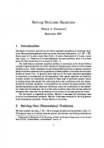
Figure 1: The exact solution of u(x,t) for the equations (1) if a0 = 1, β = α = .01.
Figure 3: The exact solution of v(x,t) for the equations (1) if a0 = 1, β = α = .01.
Figure 2: The approximate solution of u(x,t) for the first three approximation of the equations (1) if a0 = 1, β = α = .01.
Figure 4: The approximate solution of v(x,t) for the first three approximation for the equations (1) if a0 = 1, β = α = .01.
Table 2. The MVIM results of v(x, t) for the first three approximation in comparison with the analytical solution if a0 = 1, β = α = .01,and t = 20 for the solution of the system (1) with the initial conditions(15).
ditions [11]:
x -50 -40 -30 -20 -10 10 20 30 40 50
5.2
vExact -1.1204856E-7 -1.2401512E-7 -1.4991042E-7 -2.2395349E-7 -6.2401173E-7 -6.2401173E-7 -2.2395349E-7 -1.4991042E-7 -1.2401512E-7 -1.1204856E-7
vM V IM -1.12232E-7 -1.24375E-7 -1.50764E-7 -2.26833E-7 -6.46982E-7 -6.00746E-7 -2.21054E-7 -1.49052E-7 -1.23653E-7 -1.11863E-7
|vExact −vM V IM | 1.853690E-7 1.855450E-7 1.860388E-7 1.880649E-7 2.081564E-7 1.619202E-7 1.822860E-7 1.843273E-7 1.848238E-7 1.850006E-7
Solving the (1+1)-dimensional JaulentMiodek (JM) equations using MVIM
These initial conditions follow by setting t = 0 in the following exact solutions of eqs. (2): 1 1 √ u(x, t) = (c − b2 ) − b c 4 2 2 √ (6b + c)t sech( c (x + )) − 2 √ 3c (6b2 + c)t sech2 ( c (x + )), 4 2 √ v(x, t) = b + c √ (6b2 + c)t × sech( c (x + )), 2
(28)
where c and b are arbitrary constants. These exact solutions have been derived by Fan [11] using the unified algebraic method. Let us now solve the initial value problem (2) and (27) using the MVIM. To this
In this subsection, we find the solutions u(x, t), v(x, t) satisfying the (1+1)-dimensional JaulentMiodek (JM) equations with the following initial con-
E-ISSN: 2224-2880
√ 1 1 √ u(x, 0) = (c − b2 ) − b c sech( c x) − 4 2 3c 2 √ sech ( c x), 4 √ √ v(x, 0) = b + c sech( c x). (27)
298
Issue 4, Volume 11, April 2012
WSEAS TRANSACTIONS on MATHEMATICS
E. M. E. Zayed, H. M. Abdel Rahman
6{(un )x (vn ) + (un )(vn )x } −
end, we convey the basic idea of the modified variational iteration method for the equations (2), let us consider the functional iteration formula ∫
∞ ∞ ∑ 15 ∑ ( pn vn )x ( pn vn )2 ]dτ. 2 n=0 n=0
t
un+1 (x, t) = un (x, t) +
λ1 (τ )[(un )τ +
Using eqs. (31) to compare the coefficient of like powers of p then we have
0
3 9 en )xxx + (ven )(ven )xxx + (ven )x (ven )xx − (u 2 2 en )(u en )x + (u en )(ven )(ven )x } − 6{(u 3 en )x (ven )2 ]dτ, (u 2 ∫
u0 (x, t) = u(x, 0), u1 (x, t) = −
t
vn+1 (x, t) = vn (x, t) +
λ2 (τ )[(vn )τ +
en )x (ven ) + (ven )xxx − 6{(u 15 en )(ven )x } − (u (ven )x (ven )2 ]dτ. (29) 2 Making the correct functional stationary, the Lagrange multipliers can be identified as λ1 (τ ) = −1=λ2 (τ ) = −1, consequently ∫
t
[(un )τ + (un )xxx + 0
9 3 (vn )(vn )xxx + (vn )x (vn )xx − 2 2 6{un )(un )x + (un )(vn )(vn )x } − 3 (un )x (vn )2 ]dτ, 2 ∫
vn+1 (x, t) = vn (x, t) −
t
0
pn un = u0 − p
∫
t
[(
v1 (x, t) = −
[(vn )τ + (vn )xxx −
0
n=0
∞ ∑
v2 (x, t) = −
n=0 ∞ ∑
∞ ∞ ∑ 9 ∑ ( pn v n ) x ( pn vn )xx − 2 n=0 n=0
6{
∞ ∑
pn un )(
n=0
(
∞ ∑
pn un )(
n=0 ∞ ∑
∞ ∑
pn un )x +
n=0 ∞ ∑
pn vn )(
n=0
∞ ∑
pn vn )x } −
n=0
∞ ∑
3 ( pn un )x ( pn vn )2 ]dτ, 2 n=0 n=0 ∞ ∑
pn vn = v0 (x, t) − p
n=0
E-ISSN: 2224-2880
∫
t 0
∫
t 0
[(v0 )xxx − 6{(u0 )x (v0 ) +
∫
t 0
15 (v0 )x (v0 )2 ]dτ, 2
[(v1 )τ − v1 )xxx − 6{{(u0 )x (v1 ) +
(u1 )x (v0 )} + {(u0 )(v1 )x + (u1 )(v0 )x }} − 15 {(v1 )x (v0 )2 + 2(v0 )x v1 v0 }]dτ, (33) 2
pn un )xxx + ( pn vn )( pn vn )xxx + 2 n=0 n=0 n=0
(
0
3 [(u0 )xxx + (v0 )(v0 )xxx + 2
(u0 )(v0 )x } −
pn un )τ +
∞ 3 ∑
∞ ∑
t
v0 (x, t) = v(x, 0),
6{(un )x (vn ) + (un )(vn )x } − 15 (vn )x (vn )2 ]dτ. (30) 2 Applying the modified variational iteration method, we have ∞ ∑
∫
9 (v0 )x (v0 )xx − 6{u0 )(u0 )x + 2 3 (u0 )(v0 )(v0 )x } − (u0 )x (v0 )2 ]dτ, 2 ∫ t 3 u2 (x, t) = − [(u0 )τ (u1 )xxx + {(v1 )(v0 )xxx + 2 0 9 (v0 )(v1 )xxx } + {(v0 )x (v1 )xx + (v1 )x (v0 )xx } − 2 6{{u0 )(u0 )x + u1 )(u1 )x } + {(u1 )(v0 )(v0 )x + (u0 )(v1 )(v0 )x + (u0 )(v0 )(v1 )x }} − 3 {(u1 )x (v0 )2 + 2(u0 )x (v0 )(v1 )}]dτ, (32) 2
0
un+1 (x, t) = un (x, t) −
(31)
[(vn )τ + (vn )xxx −
299
The other components can be found similarly. After some reduction, we have √ 1 1 √ u0 (x, t) = (c − b2 ) − b c sech( c x) − 4 2 3c 2 √ sech ( c x), 4 √ √ t u1 (x, t) = − (c + 6b2 ){bc sech( c x) tanh( c x) 4 √ √ + 3c3/2 sech2 ( c x) tanh( c x)}, √ t2 u2 (x, t) = − (c + 6b2 )2 {bc3/2 (sech3 ( c x) + 8 √ √ √ sech( c x) tanh2 ( c x)) + 3c2 (sech4 ( c x) √ √ + 2sech2 ( c x) tanh2 ( c x))}, (34)
Issue 4, Volume 11, April 2012
WSEAS TRANSACTIONS on MATHEMATICS
E. M. E. Zayed, H. M. Abdel Rahman
√ √ v0 (x, t) = b + c sech( c x), √ √ ct (c + 6b2 )sech( c x) tanh( c x), v1 (x, t) = 2 √ c3/2 t2 v2 (x, t) = (c + 6b2 )2 {sech3 ( c x) + √ 4 √ sech( c x) tanh2 ( c x)}, (35) In this manner the other components can be easily obtained. We construct the solutions u(x, t) and v(x, t) as follows: √ 1 1 √ u(x, t) = (c − b2 ) − b c sech( c x) − 4 2 √ √ 3c t sech2 ( c x) − (c + 6b2 ){bc sech( c x) 4 4 √ √ × tanh( c x) + 3c3/2 sech2 ( c x) √ c3/2 t2 tanh( c x)} − (c + 6b2 )2 {bc3/2 8 √ √ √ ( sech3 ( c x) + sech( c x) tanh2 ( c x)) + √ √ 3c2 (sech4 ( c x) + 2sech2 ( c x) √ × tanh2 ( c x))} + ..., (36) √ √ ct c sech( c x) + (c + 6b2 ) 2 3/2 √ √ c t2 × sech( c x) tanh( c x) + (c + 6b2 )2 4 √ √ × {sech3 ( c x) + sech( c x) √ × tanh2 ( c x)} + ... (37)
v(x, t) = b +
The accuracy of the MVIM for the eqs. (2) under conditions (27) are controllable and the absolute errors are very small with the present choice of x, t. These results are listed in Tables 3, 4 and Figures 5-8. It is also clear that when more terms for homotopy analysis method are computed, the numerical results are much more closer to the corresponding exact solution.
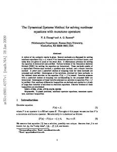
Figure 6: The approximate solution of u(x,t) for the first three approximation for the equations (2) if b = .1, c = .01. Table 3. The MVIM results of u(x, t) for the first three approximation in comparison with the exact solution if b = .1, c = .01 and t = .2 for the solution of the Eqs. (2) with the initial conditions (27). x -50 -40 -30 -20 00 00 10 20 30 40 50
uExact -0.00006878 -0.00019329 -0.00057108 -0.00186051 -0.00639517 -0.0125 -0.00638499 -0.00185728 -0.000570186 -0.00019301 -0.000068689
uM V IM -0.000068786 -0.000193286 -0.000571017 -0.00185984 -0.00638898 -0.0124967 -0.00639128 -0.00185806 -0.00057026 -0.00019302 -0.00006869
|uExact − uM V IM | 1.03236E-9 7.98438E-9 6.75572E-8 6.65449E-7 6.18910E-6 3.29510E-6 6.28541E-6 7.81587E-7 8.12470E-8 9.60074E-9 1.22044E-9
Table 4. The MMVIM results of v(x, t) for the first three approximation in comparison with the exact solution if b = .1, c = .01 and t = .2 for the solution of the eqs. (2) with the initial conditions (27). x -50 -40 -30 -20 -10 00 10 20 30 40 50
vExact 0.101348 0.103664 0.10994 0.126598 0.16484 0.2 0.164771 0.126562 0.109926 0.103659 0.101347
vM V IM 0.101347 0.10366 0.109915 0.126426 0.163784 0.199999 0.165828 0.126735 0.109951 0.103664 0.101348
|vExact − vM V IM | 1.6994901E-6 4.8481756E-6 2.5172504E-5 1.7214243E-4 1.0560166E-3 1.1865000E-6 1.0567760E-3 1.7238910E-4 2.5211635E-5 4.8552982E-6 1.7027722E-6
6 Conclusion Figure 5: The exact solution of u(x,t) for the equations (2) if b = .1, c = .01.
E-ISSN: 2224-2880
In the present paper, the modified variational iteration method (MVIM) is used to find the solutions of
300
Issue 4, Volume 11, April 2012
WSEAS TRANSACTIONS on MATHEMATICS
E. M. E. Zayed, H. M. Abdel Rahman
[4] S. Abbasbandy, A new application of He’s variational iteration method for quadratic Riccati differential equation by using Adomian’s polynomials, J.Comput. Appl. Math., Vol.207, 2007,pp. 59-63. [5] S. Abbasbandy, The application of homotopy analysis method to nonlinear equations arising in heat transfer, Phys. Lett. A., Vol.360, 2006, pp. 109-113. [6] M. A. Abdou, The extended F- expansion method and its application for a class of nonlinear evolution equations, Chaos Solitons and Fractals, Vol.31, 2007, pp. 95–104. [7] A. H. A. Ali, The modified extended tanhfunction method for solving coupled KdV equations, Phy. Letters A., Vol.363, 2007, pp. 420– 425. [8] A. K. Alomari, M. S. M. Noorani, R. Nazar, The homotopy analysis method for the exact solutions for the K(2,2), Burgers and Coupled Burgers equations, Appl. Math. Sci., Vol.2, 2008, pp. 1963–1977. [9] C. Chun, H. Jafari and Y.Il Kim, Numerical method for the wave and nonlinear diffusion equations with the homotopy perturbation method,Compu. Math. Appl. , Vol.57, 2009, pp. 1226- -1231. [10] R. Conte, J. M. Musette, The modified extended tanh-function method for solving coupled Kdv equations, Phy. Letters A., Vol.363, 2000, pp. 420-425. [11] E. G. Fan, Uniformly constructing a series of explicit exact solutions to nonlinear equations in mathematical physics, Chaos Solitons and Fractals Vol.16, 2003, pp. 819–839. [12] E. G. Fan, Extended tanh function method and its applications to nonlinear equations, Phys. Letters A, Vol.277, 2000, pp. 212–218. [13] A. Ghorbani, J. Saberi Nadjafi, He’s homotopy perturbation method for calculating Adom ian Polynomials,Int. J. Nonlinear Sci. Numer. Simul., Vol.8, 2007, pp. 229-232. [14] A. Ghorbani and S. Nadjafi, Exact solutions for nonlinear integral equations by a modified homotopy perturbation method, Comp. Math. Appl., Vol.56, 2008, pp.1032-1039. [15] J. H. He, Variational iteration method-a kind of nonlinear analytical technique: some examples, Int.J. Nonlinear Mech. , Vol.34, 1999, pp. 699– 708. [16] J. H. He, A coupling method of homotopy technique and perturbation technique for nonlinear problems, Int.J.Nonlinear Mech., Vol.35, 2000, 1: pp. 37–43.
Figure 7: The exact solution of v(x,t) for the equations (2) if b = .1, c = .01.
Figure 8: The approximate solution of v(x,t) for the first three approximation for the equations (2) if b = .1, c = .01. the nonlinear coupled equations in the mathematical physics via the (1+1)-dimensional Ramani equations and the (1+1)-dimensional Jaulent-Miodek (JM) equations together with the initial conditions. It can be concluded that the MVIM is very powerful and efficient in finding the exact solutions for wide classes of problems. It is worth pointing out that the MVIM presents rapid convergence solutions.
References: [1] T. A. Abassy, M. A. El-Tawil, H. K. Saleh, The solution of KdV and MKdV equations using Adomian Pade approximation,Int. J. Nonlinear Sci. Numer. Simul., Vol.5,2004, pp. 327–339. [2] K. Abbaoui, Y. Cherruault, V. Seng, Practical formulae for the calculus of multivariable Adomian polynomials,Math. Comput. Modelling Vol.1, 1995,pp 89–93. [3] K. Abbaoui, Y. Cherruault, The decomposition method applied to Cauchy problem, Kybernetes, Vol.28, 1999, pp. 68–74. E-ISSN: 2224-2880
301
Issue 4, Volume 11, April 2012
WSEAS TRANSACTIONS on MATHEMATICS
E. M. E. Zayed, H. M. Abdel Rahman
[17] J. H. He, New interpretation of homotopy method, Int. J. Modern Phys. B , Vol.20, 18, 2006, pp. 2561-2568. [18] J. H. He, The homotopy perturbation method for nonlinear oscillators with discontinuities, Appl.Math. Comput., Vol.151, 2004, pp. 287–292. [19] J. H. He, A coupling method of homotopy technique and perturbation technique for nonlinear problems, Int.J.Nonlinear Mech., Vol.35 ,2000, pp. 37–43. [20] J. H. He, New interpretation of homotopy method, Int. J. Modern Phys. B, Vol. 20, 2006, pp. 2561–2568. [21] J. H. He, Homotopy perturbation method for bifurcation of nonlinear problems,Int. J. Nonlinear Sci., Vol.6, 2005, pp. 207–208. [22] J.H.He, The homotopy perturbation method for nonlinear oscillators with discontinuities ,Appl.Math. Comput, Vol.151, 2004, pp. 287-292. [23] H. C. Hu, Q. P. Liu, New Darboux transformation for Hirota- Satsuma coupled KdV system, Chaos Solitons and Fractals, Vol.17, 2003, pp. 921–928. [24] M. Inokuti, H. Sekine and T. Mura, General use of the Lagrange multiplier in nonlinear mathematical physics, In:S. Nemat-Nasser(Ed.), Variational method in the mechanics of solids. Pergamon press,New York 1978, pp. 156–162. [25] W. Malfliet, W. Hereman, The tanh method I: exact solutions of nonlinear evolution and wave equations, Phys. Scripta Vol.54, 1996, pp. 563– 568. [26] W. Malfliet, The tanh method II: Perturbation technique for conservative system,Phys. Scripta, Vol.54, 1996, pp. 569–575. [27] A. Molabahrami, F. Khani, S. Hamedi-Nezhad, Soliton solutions of the two- dimensional KdVBurgers equation by homotopy perturbation method, Phys. Lett. A , Vol.370, 2007, pp. 433– 436. [28] M. A. Noor, K. I. Noor and S. T. Mohyud-Din, Modified variational iteration technique for solving singular fourth-order parabolic partial differential equations, Nonlinear Analysis: Theo., Meth. Appl., Vol.71, 2009, (12): pp.630–640. [29] S. T. Mohyud-Din, M. A. Noor and K. I. Noor, Traveling wave solutions of seventh-order generalized KdV equations using He’s polynomials, Int. Sci. Numer. Simul., Vol.10, 2009, (2):pp. 227-234. [30] M. A. Noor and S. T. Mohyud-Din, Variational iteration method for solving higher-order nonlinear boundary value problems using He’s polynomials,em Int. J. Nonlinear Sci. Numer. Simul., Vol.9, 2008, pp. 141-156. E-ISSN: 2224-2880
[31] M. A. Noor and S. T. Mohyud-Din, Variational iteration method for solving fifth-order boundary value problems using He’s polynomials. Math. Prob. Eng., 2008, doi:10.1155/954794. [32] J. I. Ramos, On the variational iteration method and other iterative techniques for nonlinear differential equations, Appl. Math. Comput., Vol.199, 2008, pp.39–69. [33] M. Tatari, M. Dehgham, On the convergence of He’s variational iteration method, J. Comput. Appl. Math., Vol.207 , 2007,pp 121–128. [34] M. L. Wang and X. Z. Li, Applications of Fexpansion to periodic wave solutions for a new hamiltonnian amplitude equation, Chaos, Soliton and Fractals, Vol.24, 2005, pp.1257–1268. [35] W. Wu, S.J. Liao, Solving solitary waves with discontinuity by means of homotopy analysis method, Chaos Solitons and Fractals, Vol.26, 2005, pp. 177-185. [36] Y. Yu, Q. Wang, H.Zhang, The extended Jacobi elliptic function method to solve a generalized Hirota- Satsuma KdV equations, Chaos Solitons and Fractals, Vol.26, 2005, pp. 1415–1421. [37] E. Yusufoglu, A. Bakir, Exact solutions of nonlinear evolution equations, Chaos, Solitons and Fractals, Vol.37, 2008, pp. 842–848. [38] E. M. E. Zayed, H. A. Zedan and K. A. Gepreel, Group analysis and modified extended tanhfunction to find the inveriant solutions and soliton solutions for nonlinear Eular equation, Int. J. Nonlinear Sci. Numer. Simul. Vol.5, 2004, pp. 221–234. [39] E. M. E. Zayed, T. A. Nofal and K. A. Gepreel, Homotopy perturbation and Adomian decomposition methods for solving nonlinear Boussinesq equations, Commun. Appl. Nonlinear Anal., Vol. 15, 2008, pp. 57–70. [40] J. L. Zhang, M. L. Wang, Z. D. Fang, The improved F- expansion method and its applications, Phy. Letters A, Vol.350, 2006, pp. 103–109.
302
Issue 4, Volume 11, April 2012