LSP when there is no other way to route the new one. Our ... the widely known Constrained Shortest Path First (CSPF) ..... mathematics ISBN 0 471 90854 1.
IEEE ICCCN 2000
1
On–demand optimization of label switched paths in MPLS networks ´ Alp´ar J¨ uttner, Bal´azs Szviatovszki, Aron Szentesi, D´aniel Orincsay, J´anos Harmatos Abstract— Multiprotocol Label Switching technology provides efficient means for controlling the traffic of IP backbone networks and thus, offers performance superior to that of traditional Interior Gateway Protocol (IGP) based packet forwarding. However, computation of explicit paths yielding optimal network performance is a difficult task; several different strategies can be thought of. In this paper we propose a novel approach for the optimal path selection of new label switched paths (LSPs). Our method is based on the idea that we allow the re-routing of an already established LSP when there is no other way to route the new one. Our optimization algorithm is based on an Integer Linear Programming (ILP) formulation of the problem. We show by numerical evaluation that our method significantly improves the success probability of setting up new LSPs by extending the widely known Constrained Shortest Path First (CSPF) algorithm with the ILP-based re-routing function. Although the task itself is NP-hard, our heuristic solution provides efficient solutions in most practical cases. The proposed algorithm is aimed to be implemented primarily in a network operation center. However, with the restriction that only LSPs starting from the optimizing Label Edge Routers can be re-routed, the algorithm can be implemented directly in edge routers themselves. Keywords— Multiprotocol Label Switching, traffic engineering, optimization, routing, path selection
I. Introduction
M
PLS provides a number of traffic engineering features for Internet Service Providers to have precise control over the placement of traffic flows within their networks. Operators can configure explicit Label Switched Paths (LSPs) with primary and hot-standby secondary MPLStunnels, define loose and strict hops, configure preemption based on setup- and holding-priority levels and assign resource class affinity attributes (administrative groups or colors simply) to certain resources. These features provide handy control options for operators to specify the paths of traffic flows in their network. There are many ways how LSPs can be established in an MPLS network. The simplest method is when the operator sets up so called default or topological LSPs. In this case the path of the LSP is determined solely by the egress router’s IP address and by the routing tables of intermediate transit routers (i.e., the LSP path is identical to the IGP path). In a bit more complex case, an operator can specify explicitly some loose or strict hops for the LSP. For example between San Jose and New York a primary and hot-standby secondary MPLS-tunnel of an LSP can be routed towards Chicago and Houston, respectively. In Ericsson Research, Traffic Analysis and Network Performance Laboratory, POB 107, H-1300 Budapest, Hungary. E-mail: {Alpar.Juttner, Balazs.Szviatovszki, Aron.Szentesi, Daniel.Orincsay, Janos.Harmatos }@eth.ericsson.se Fax: +36-1-437 7219 Phone: +361-437 7631
this method the LSP still uses the IGP path between the specified hops. When the operator optimizes global LSP placement with the help of a central Traffic Engineering (TE) tool, explicit paths will be completely specified with strict hops. When the underlying interior routing protocol is extended with an MPLS bandwidth reservation related information distribution component, Label Edge Routers can conduct on-demand constrained routing (CSPF) calculations for each LSP, thus automating the constrained LSP establishment procedure. The LER routing algorithm can be implemented in such a way that it computes paths taking into account the explicit hop and hop limit constraints defined by the operator. Edge routers use RSVP [1] or LDP [2] signaling to establish LSPs on explicit paths. In both protocols two kinds of priorities are supported: setup and holding priorities. Bandwidth reservations are counted on each interface for each holding priority level separately. When a new LSP is to be established, its setup priority is compared to the unreserved bandwidth of the corresponding holding priority level. When there is not enough resource available at that level, the LSP setup fails, otherwise some local algorithm determines which lower priority LSPs will be preempted. In case a network uses only topological LSPs, preempted tunnels will be blocked, since they have no other choice to take. However, when CSPF is used, the preempted ones can have another chance to fit into alternate paths not occupied by higher priority LSPs. By using CSPF it can still occur that for a new LSP there is not enough bandwidth available at its own priority level. In this case the LER have no other chance, but to block the LSP. In an operational MPLS network, the CSPF computations implemented in edge routers automate LSP setups. However, edge routers have only local information about the network resources. These local routing decisions made in LERs may result in a degraded global network performance on the long run. One solution for this is to perform periodical (not too frequent, e. g. daily or weekly) global re-optimization of LSPs with a centralized off-line network optimization tool [3]. Another approach is to make the CSPF computation itself more intelligent by implementing a kind of preventive strategy. Concepts used in dynamic routing methods proposed for ATM networks (see e. g. [4], [5]) could be re-used to improve LSP path selection performance, by implementing local strategies that result in globally near-optimal solutions. Recently [6] proposed the concept of minimum interference routing that is based on this idea. The newly developed algorithm presented in this paper
IEEE ICCCN 2000
2
is intended to be used in the case when on-demand CSPF based LSP setup in a Label Edge Router fails. Such a failure can happen when there is not enough bandwidth since LSPs of the same (or higher) priority level occupy network resources. This kind of situation may arise even if a preventive routing strategy is used, although at higher network utilization levels. In such failure situations, supposing that the operator wants to fit in the new LSP, a quick re-optimization of as few LSPs as possible is more preferable than an immediate global re-optimization of all LSP paths. A special case of the above strategy is to allow the re-configuration of only a single LSP. This requires the smallest amount of management interactions, while still providing the efficient solution to overcome the problem arose from the CSPF failure. Thus, our proposed algorithm implements such a failure triggered partial re-optimization strategy in which we try to re-route only one LSP. The rest of the paper is structured as follows. In Section II we formulate the problem. We describe our algorithm in Section III by presenting its three main parts. We use an Integer Linear Programming based solution in the algorithm, for which an efficient solution is presented in Section IV. In Section V we present numerical results, and finally in Section VI conclusion are drawn. II. Problem statement As it was outlined in the introduction, the task we address in this paper is to select a single LSP that can be re-routed in order to be able to establish a new one. The exact definition of the problem is therefore the following: • We are given all the information on the network topology and status, including the bandwidth reservations and actual paths of currently established Label Switched Paths (LSPs), (we will refer to these LSPs as old ones) • We have a new LSP request from, say, node s to node t with bandwidth demand b. • Assume that there is no s −→ t path with sufficient unreserved bandwidth for accommodating the incoming request b (otherwise the problem is trivially solved by CSPF). Our task is to release sufficient bandwidth on some ’bottleneck’ links (i. e., where the unreserved bandwidth bf is less than b) by re-routing a single LSP, so that we can set up the new LSP.
The non-trivial problem here is to find an existing LSP that can be re-routed so that after the re-routing the new LSP can also be established. This problem is NP-hard [7], therefore we propose a heuristic algorithm for its solution. Since we need path information of already established LSPs, the re-optimization can be done primarily in a network operation center rather than in the edge routers themselves. The complexity of the optimization algorithm also calls for this solution. However, theoretically, with limited scope, the algorithm can be implemented in Label Edge Routers, as well. The restriction in this case is that only LSPs starting from the optimizing LER can be re-routed.
III. The Algorithm The main purpose of this algorithm is to re-route an LSP that is already established, so that the new LSP can be placed into the network. Fig. 1 depicts the flow chart of the algorithm. Start
Filtering
Select LSP
TwoPath (ILP)
Correct Paths? Yes
No
More LSPs?
Yes
No
Finish
Finish
(Success)
(Failure)
Fig. 1. Flowchart of the optimization algorithm
The aim of the first function is to filter the LSPs. The simplest approach would be to try to re-route all established LSP one by one. In small networks this is reasonable, but in larger ones it is unacceptable, because of the large number of LSPs. Consequently, it is necessary to decrease the number of such established LSP to be examined. There can be such old LSPs that are even if completely released, the establishment of the new LSP will still not be possible. It is of no use to try to re-route such LSPs. At the second part of the algorithm we take the candidate re-routable LSPs one by one, and execute an ILP based function called TwoPath. This function tries to establish the new LSP and re-route the selected old LSP simultaneously. If the TwoPath function finds a solution, the optimization is complete, so the whole algorithm finishes. If TwoPath could not find any re-routable old LSP, it finishes with failure. In the rest of this section the main parts of the algorithm are described in more detail. A. Filtering The aim of filtering is to reduce the number of LSPs for which the TwoPath algorithm is called. We implemented three different filters. The first filter examines the so-called bottleneck links. Bottleneck is such a link that does not have enough available bandwidth for the new LSP. First, the filter calculates the minimal number of bottlenecks for the new LSP by Dijkstra’s shortest path algorithm with the following weight function: 1 if edge e has not enough available bandwidth for the new demand, w(e) = 0 otherwise.
IEEE ICCCN 2000
Dijkstra’s algorithm aims to avoid the bottlenecks, therefore the resulting shortest path will contain the minimal number of bottlenecks. Let nmin denote this minimum value. If a configured LSP contains less bottlenecks than nmin , then rerouting this LSP will surely not help the configuration of the new LSP, because at least on one link the available unreserved bandwidth will be less than the bandwidth requested by the new LSP. The basic idea behind the second filter is the following. Starting in any direction from the source node towards the destination, we will bump against a bottleneck link. Those bottleneck links that are reachable from the source node directly (i.e. without passing another bottleneck link), are called first bottleneck links. The LSP to be rerouted has to use one of the first bottleneck links in order to be able to establish the new demand. This filter uses the same weight function as the one above and searches the first bottleneck links in the following manner: 1. It searches for a shortest path. 2. It searches for the first bottleneck link of this path, deletes it from the graph temporarily, and stores it into a list. 3. It repeats the first two steps until there is no path between the source and destination nodes of the LSP demand. When all possible first bottleneck links are found, we filter out such old LSPs which do not use any of the bottleneck links of the list. The third filter checks whether the unreserved bandwidth of the bottleneck link — after re-routing the selected old LSP — will be large enough to accommodate the new demand. This filter precludes the possibility of re-routing those configured LSP which does not facilitate the placement of the new demand into the network. B. Select LSP The aim of the TwoPath function is to examine whether two LSPs — an old one and the new one — can be established simultaneously. This function selects old LSPs one by one, and calls the TwoPath function. In our implementation, first those old LSPs are examined that have the same ingress router as the new one. The reason for this is simple: our algorithm identifies an old LSP to be re-routed, and determines the new path for both the old and the new LSP. In case the algorithm is implemented in a central place of the network (e.g., in a TE tool), the result of optimization should be communicated back to the network. If the ingress router of both LSPs are the same, the TE tool should order a single LER to do the change, in this way simplifying the whole re-routing procedure. Of course, when there is no LSP with common ingress, all the rest of the LSPs need to be examined. C. TwoPath In this section we formulate an Integer Linear Program that solves the establishment of two LSPs — the new LSP and an old one — simultaneously. Instead of the MPLS terminology, for LSPs we use the term paths, that better fits the mathematical context.
3
We examine the problem of routing two paths. The network is represented by a directed graph N = (V, E) with the set V of vertices and the set E of edges. Two pair of nodes s1 , t1 ∈ V and s2 , t2 ∈ V are also given, representing the source and destination nodes of the two paths. The two paths to be routed can have different capacities. Therefore we classify the edges of the graph with the help of three subsets E1 , E2 and Eb of E. Edges in E1 , and E2 have enough capacity to accommodate the first path and the second path, respectively. (An edge can be in both sets at the same time). Edges in Eb can not accommodate the two paths together. With these notations our task is to find two paths P1 and P2 from s1 to t1 and from s2 to t2 such that P1 ⊆ E1 , P2 ⊆ E2 and P1 ∩ P2 ∩ Eb = 0, that is, the path Pi can use only the edges of Ei and furthermore, the edges which are used by both paths must not be in Eb . By setting Eb = E, we can force the algorithm to find disjoint paths. This problem can be formulated as an integer linear program in the following way. We seek the integer numbers xe1 ∈ {0, 1}, e ∈ E1 and xe2 ∈ {0, 1}, e ∈ E2 satisfying the conditions:
X
xe1 −
e∈ρ(v)∩E1
X
e∈ρ(v)∩E2
X
xe1 ≥ 0 xe2 ≥ 0
∀e ∈ E1 (1a) ∀e ∈ E2 (1b)
xe1 = δv,t1 − δv,s1
∀v ∈ V
(1c)
xe2 = δv,t2 − δv,s2
∀v ∈ V
(1d)
e∈δ(v)∩E1
xe2 −
X
e∈δ(v)∩E2
xe1 + xe2 ≤ 1
∀e ∈ Eb , (1e)
where ρ(v) and δ(v) are the sets of the incoming and the outgoing edges of the node v and δi,j is 1 or 0 according to whether i is equal to j or not. We can extend this problem to an optimization problem by assigning two cost functions c1 , c2 : E −→ R+ to the edges. In this case let the cost of a path Pi be the sum of the corresponding costs of the edges of Pi . We are looking for the paths which satisfy the above constraints and minimize the sum of the cost of the two paths. Using the above ILP notations our task is to find the integer vectors x1 and x2 which satisfy (1a)-(1e) and approach X X c1 (e)xe1 + c2 (e)xe1 (2) min e∈E1
e∈E2
with respect to the constraints. IV. ILP Solution In this section we describe how to solve efficiently the ILP problem formulated in the previous section. Basically, any ILP software package can be used. The ILP solver packages use the so-called branch&bound technique [8] to solve an integer program. In our case this means solving several times the problem (2),(1a)-(1e) with some predefined variables but without the integrality constraints.
IEEE ICCCN 2000
4
We tested the lp solve package [9] and it gave good results. However, we found that for larger graphs lp solve can be slow. This comes from the fact that lp solve uses the simplex method to solve the LP problem, which can be inefficient. Without the integrality constraint this problem is a Multicommodity Flow Problem [10] with two commodities, so we can improve our algorithm by replacing the simplex method with a more efficient one. We propose to use the so called Column Generation Procedure [8], that we describe with the help of the following model: It is well-known that the optimal flows can be decomposed into paths. (Since we neglected the integrality constraint a flow can be routed on more than one path). We intend to find directly this decomposition. For this, let P1 and P2 be the sets of all s1 —t1 and s2 —t2 paths in E1 and E2 respectively. In this formulation we have a variable αP for all paths P ∈ P1 ∪ P2 . Using these notations our task is to
min
X
c1 (P )αP +
P ∈P1
X
c2 (P )αP
(3a)
P ∈P2
subject to X
X
αP +
P ∈P1 ,e∈P
αP ≥ 0
∀P ∈ P1 ∪ P2
(3b)
αP ≤ 1
∀e ∈ Eb
(3c)
P ∈P2 ,e∈P
X
αP = 1
(3d)
αP = 1.
(3e)
P ∈P1
X
P ∈P2
This LP has only |Eb | + 2 constraints but the number of variables are typically enormous. However, it follows from a standard linear programming consideration that there exists an optimal solution having only at most |Eb |+2 nonzero variables and we can find it very efficiently without storing the entire huge constraint matrix using the so-called column generation procedure. In order to use this method we transform (3c) to equality constraints by adding slack variables. X
αP +
P ∈P1 ,e∈P
X
ze ≥ 0 e
αP + z = 1
∀e ∈ Eb ∀e ∈ Eb
(3c’)
P ∈P2 ,e∈P
Because the method needs an initial solution we also modify the constraints (3d) and (3e) X
s 1 , s2 ≥ 0 αP + s1 = 1
(3d’)
αP + s2 = 1.
(3e’)
P ∈P1
X
P ∈P2
Now we can easily obtain an initial solution to the problem by setting all variables z e and s1 , s2 to 1 and the rest of the variables to 0. If the variables s1 and s2 have sufficiently large costs then the optimal solution will avoid these variables if possible. The column generation procedure uses the primal simplex method to get the optimal solution from the initial solution by a sequence of “pivot operations”. This method stores a so-called basis structure which is a set of |Eb | + 2 variables such that each non-zero element of the current solution is one of these variables. In each iteration it chooses a new variable which enters the basis, modifies the current solution and chooses a leaving variable. Fortunately, in our special case we do not need to scan all columns to choose the entering variable but it can be done by using Dijkstra’s shortest path algorithm. The reader is referred for example to [10] for a detailed description of this procedure. A good and in-depth survey on the linear programming background can be found in [8]. To get an integer solution to the problem (3a)-(3e) we establish a recursive branch&bound procedure which is called with the sets E1 , E2 , Eb and a bounding number B as input. As the output, it either states that there exists no feasible integer solution to the problem (3a)-(3e) whose cost is less than B, or it provides the optimal integer solution with cost less than B. The branch&bound procedure first solves the problem (3a)-(3e) using the aforementioned column generation procedure. If there are no feasible flows, or the cost of the optimal flows is greater than B, then there will be no sufficient integer solution, so the procedure can state this as an output. It is also a straightforward consideration that if the two flows resulting from the column generation procedure do not use any edge of Eb together, then they must be integer flows, i.e., they are paths. Obviously, in this case this is an optimal solution, so branch&bound can return this. Finally, if the flows share an edge e ∈ Eb then we do two recursive calls of branch&bound with the sets E1 \ {e}, E2 , Eb , and E1 , E2 \ {e}, Eb , respectively. When calling branch&bound with the first sets cost B is used as the bounding parameter. In case it finds an integer solution whose cost C is less than B, then C is used as the bounding parameter at the second call of branch&bound . When the first branch did not find an integer solution, cost B is used at the second call. Our task is to have an integer solution to the LP problem, or to know that such solution does not exist. Therefore we call branch&bound with the original sets E1 , E2 , Eb and +∞ as the bounding parameter. If none of the recursive calls provide a feasible solution, then we can state that there exists no integer solution. Otherwise, one of the solutions provided by the recursive call will give us the best integer solution. By using the branch&bound method and the column generation procedure we get a more efficient method then the one implemented in an ILP software package.
IEEE ICCCN 2000
5
V. Numerical results We have conducted extensive numerical investigations in order to show the real improvements resulting from the use of our algorithms. Our goals with the numerical evaluation were twofold: • first, we wanted to get some insight to the computational efficiency and, therefore, the practical applicability of our algorithms. Recall that our basic problem is NP-hard; it is therefore essential to check the limits of our ILP-based solution heuristic. • second, we wanted to quantify the actual performance gain resulting from the use of our proposed algorithm in a practical network. Besides showing the trivial fact that allowing a re-routing of an existing LSP — in case simple CSPF-based routing fails — indeed improves the success probability of a new LSP setup, we wanted to characterize the network-level gain in a real-world system. A. Computational efficiency For the measurement of the running times of the algorithm we generated random network topologies of 50, 100, 150 and 200 nodes. We have run our column-generation based algorithm for several times using Sun UltraSparc 5 computers, and calculated average running times for the different examples. For reference, we solved the same problem instances with the lp solve [9] package as well. Table I summarizes the results.
Lp solve Column Generation
50 Nodes 0.14s 0.06s
100 Nodes 1.4s 0.5s
150 Nodes 4.6s 1.8s
200 Nodes 8.2s 5.2s
We, therefore, have decided to use a simple but effective evaluation strategy. We created randomly generated traffic situations in an example network topology. This means that we have loaded the network to a certain extent with randomly placed LSPs having random bandwidth values. On these random traffic situations we evaluated the probability of being able to add a single new LSP by trying to establish several new ones, one after another. All the new LSPs were tried with random capacity, origin and destination nodes, using the same initial traffic situation. This test has been conducted for several different network load values, resulting in a series of probabilities describing the quality of the routing strategy at different traffic levels. In order to have practically relevant results we have decided to base our investigations on the AT&T IP Backbone. It contains 25 backbone nodes and 88 links, resulting in an average 3.52 node degree. The exact topology and capacity values of this network (and of many others) are publicly available [11]. The main purpose of the first round of our simulations was to determine the difference in successful LSP establishment probability between the constrained shortest path first (CSPF) algorithm and our advanced ILP based algorithm that allows the re-routing of an already established LSP in the case when CSPF fails. First, we loaded the network to a certain level by generating LSPs randomly between all nodes. This traffic situation is characterized by the total throughput, i.e., the sum of all established LSPs’ bandwidth. In order to approximate the success probability, we randomly generated several new LSPs, and tried to route them both with the CSPF method and with our optimized method, all of them in the same traffic situation. As we can see in Fig. 2, the success prob100
Two important conclusions can be drawn from the results. The first — and probably most important — message is that our ILP-based solution scales very well for practical network sizes (150-200 nodes), although the problem itself is NP-hard. Secondly, the results show that — with respect to running times — our column-generation based procedure performs significantly better than lp solve. B. Performance evaluation Several different approaches are used for the performance evaluation of routing strategies. For example, Plotkin [4] proposes an analytical approach for this purpose. Another method is to use discrete event simulation, assuming a stochastic process for the arrival of demands [5]. In our case, it was hard to find a tractable analytical approach that can be used to obtain practical results. Discrete event simulation is again out of the scope because of the lack of a well-established and justified LSP demand arrival model in the case of MPLS.
Success Probability [%]
TABLE I Average Running Times
80 60 40 20 0 25000
CSPF Optimized 30000 35000 40000 Sum of LSPs [Mbit/s]
45000
Fig. 2. Efficiency of Optimization in Case of Same Initial State
ability of our ILP-based method is always above of CSPF’s, as it trivially has to be, considering the basic principle of our method. (Giving another chance for the set-up when CSPF failed will definitely not decrease the success probability). More importantly, however, Fig. 2 shows that the performance gain of our optimized method is quite significant when compared to the original CSPF method. Applying our proposed re-routing strategy, however, im-
IEEE ICCCN 2000
6
100
Total Load [%]
80 60 40 20 0 25000
Success Probability [%]
100
60 40 20
45000
Fig. 3. Total Load of Network
We might expect that this phenomenon will adversely effect the success probability of our optimized method. However, as we see in Fig. 4, this effect is significant only in the range of higher network load values. The optimized method retains its significant advantage above CSPF until the utilization level of the network reaches 70% (observe that this is a rather high load value, considering the achievable 20% success probability). As we mentioned in the introduction, our optimization method was originally intended to be a part of a central network traffic engineering tool, where the optimization can have global access to information on all LSPs. It is, however, possible to base the optimization on local information only and implement the algorithm right into the routers of the network. This way, we restrict ourselves to be able to re-route only those LSPs that originate from this particular router. Fig. 5 shows that we can expect some gain from using the optimized method even in this case. VI. Conclusion The algorithm described in this paper is based on the idea that in the case when there is insufficient capacity in
CSPF Optimized 30000 35000 40000 Sum of LSPs [Mbit/s]
45000
Fig. 4. Efficiency of Optimization in Case of Different Initial States
100 80 60 40 20 0 25000
CSPF Optimized 30000 35000 40000 Sum of LSPs [Mbit/s]
80
0 25000
Success Probability [%]
plies that LSPs originally routed on shortest paths will possibly be directed to longer bypasses in order to accommodate new incoming requests. This means that, when applied several times, our optimization method might result in a higher global network load (link utilization) for a certain throughput than the original CSPF. Therefore, in our second simulation phase we investigated the case when an operator uses either CSPF or our optimized method for LSP establishment all the time from day one. This means that the initial loading of the networks to a certain throughput level was achieved in different ways for the two curves. In the first case, all LSPs were established by CSPF, while for the optimized method, from the very beginning LSPs were routed by our ILP-based method whenever CSPF failed. Results displayed in Fig. 3 seem to prove our theoretical expectations: use of the optimized method indeed generates higher network load for the same throughput.
CSPF Optimized 30000 35000 40000 Sum of LSPs [Mbit/s]
45000
Fig. 5. Efficiency of Optimization with Local LSPs Only
the network to set up a new LSP, we try to free some capacity on bottleneck links by re-routing one of the established LSPs. We have proposed a systematical method for finding such an LSP. We have developed an ILP-based solution that can efficiently solve this problem for practical network sizes. Our empirical results show that the proposed algorithm significantly improves the probability of successful LSP establishment. Our future investigations will include the development of additional heuristics improving the running time of the algorithm. One idea can be to sort LSPs based on a probability measure that describes the probability of how easy will be the routing of the new LSP if that particular old LSP is re-routed. Another direction of future work is to investigate the more complicated problem of allowing the re-routing of not only a single, but more LSPs. References [1] Daniel O. Awduche, Lou Berger, Der-Hwa Gan, Tony Li, George Swallow, Vijay Srinivasan, Extensions to RSVP for LSP Tunnels, Internet Draft, September 1999 [2] Bilel Jamoussi, Editor, Constraint-Based LSP Setup using LDP, Internet Draft, February 1999 [3] D. Awduche, J. Malcolm, J. Agogbua, M. O’Dell, J. McManus, Requirements for Traffic Engineering Over MPLS, Request for Comments 2702, September 1999 [4] Serge Plotkin, Competitive Routing of Virtual Circuits in ATM
IEEE ICCCN 2000
Networks, IEEE Journal of Selected Areas in Communications, Vol. 13, No. 6, August 1995, pp. 1128-1136 ´ am Magi, G´ ´ [5] Ad´ abor Nagy, Aron Szentesi, Bal´ azs Szviatovszki, Analysis of link cost functions for PNNI routing, 6th IFIP Workshop on Performance Modelling and Evaluation of ATM Networks, Ilkley, 1998. [6] Murali Kodialam, T. V. Lakshman, Minimum Interference Routing with Applications to MPLS Traffic Engineering, IEEE INFOCOM 2000, Tel Aviv, Israel, 2000. [7] M. R. Garey, D. S. Johnson, Computers and Intractability: A Guide to the Theory of NP-Completeness 1979, Freeman, San Francisco, CA. [8] Alexander Schrijver, Theory of Linear and Integer Programming 1986, Jowh Wiley&Sons, Wiley-Interscience series in discrete mathematics ISBN 0 471 90854 1 [9] Michel Berkelaar, Jeroen Dirks, lp solve 2.2, ftp://ftp.es.ele.tue.nl/pub/lp solve [10] Ravindra K. Ahuja, Tomas L. Magnanti, James B. Orlin, Network Flows 1993, PRENTICE HALL, Upper Saddle River, New Jersey 07458. [11] Russ Haynal, Russ Haynal’s ISP Page, http://navigators.com/isp.html
7